Assessment of Observed and Projected Extreme Droughts in Perú—Case Study: Candarave, Tacna

Abstract

Droughts have always been one of the most dangerous hazards for civilizations, especially when they impact the headwaters of a watershed, as their effects can spread downstream. In this context, observed droughts (1981–2015) and projected droughts (2016–2100) were assessed in Candarave, the headwaters of the Locumba basin. Regarding observed droughts, SPI-3 and SPEI-3 detected seven extreme droughts (1983, 1992, 1996, 1998, 2010, 2011, and 2012), with the most intense occurring in 1992 and 1998. SPI-6 and SPEI-6 identified the same extreme drought events, highlighting 1992 as the most intense. Additionally, it was concluded that the VCI also detected the droughts identified by the SPEI; however, a more detailed analysis of its use is necessary due to the limited availability of suitable satellite images in the area. On the other hand, a high-resolution dataset of climate models from the sixth phase of the Coupled Model Intercomparison Project (CMIP6) under the SSP3-7.0 scenario was used to project future droughts. Of the models in that dataset, CanESM5, IPSL–CM6A–LR, and UKESM1–0–LL did not perform well in the study area. SPI and SPEI projected more than ten episodes of extreme drought, indicating that extreme droughts will become more frequent, severe, and intense in the last 30 years of this century.

1. Introduction

Drought is an atmospheric natural regional phenomenon associated with terrestrial climate variability, and therefore, it has a temporal periodicity [1]. Drought generally occurs when an area experiences a deficit of precipitation over a period of time, leading to water shortages [1,2]. As a hazard, drought can be classified into four types: meteorological or climatological, agricultural or agrometeorological, hydrological, and socioeconomic drought [1,3]. However, some authors include ecological drought in this classification [4,5]. The early stages of accumulated lack of atmospheric precipitation are considered as meteorological drought; therefore, its analysis is the basis for early warning of subsequent droughts [1,6]. A longer persistence of this precipitation deficit will rapidly impact agriculture activities and water bodies when accompanied by temperatures exceeding the usual levels, high winds, and low relative humidity [1].

Nowadays, due to climate change, drought is one of the most concerning hazards affecting human society and the environment [6]. Climate change is expected to increase the water cycle with greater evapotranspiration and less precipitation [7], raising the probability and frequency of extreme hydrological events such as droughts [2,6,7]. Climate change interacts with droughts in many ways. Less rainfall, over time, can cause surface water sources and aquifers to dry up. This, in turn, can lead to water shortages for human activities and agricultural systems [8,9]. It can also damage flora and affect fauna. However, the local climate of a specific region determines the intensity and temporality of climate change effects [10,11]. To assess these changes in the future climate and the consequent drought patterns, the Global Climate Models (GCMs) from the Coupled Model Intercomparison Project (CMIP) are the basis [6,9].

Moreover, drought indices are commonly used to explore, characterize, and study different features of these events [1,12,13], providing decision-makers with crucial information to develop an early warning program that can mitigate drought’s impacts [14]. The Standardized Precipitation Index (SPI) and the Standardized Precipitation Evapotranspiration Index (SPEI) are the most commonly used [15]. The SPI calculation is based exclusively on precipitation data, making it advantageous in areas lacking other variables. However, it does not consider other variables influencing droughts, such as temperature [16]. On the other hand, SPEI calculation is based on the accumulated difference between precipitation (P) and potential evapotranspiration (PET) [14]. Therefore, considering that the increase in evaporation caused by global warming has a significant impact and must be considered for an accurate assessment of drought in the context of climate change, SPEI becomes advantageous than SPI [3]. Thus, considering the advantages and disadvantages of each mentioned index, assessing their regional applicability, especially regarding climate change, is essential and needs further discussion [15].

Sometimes, the low density of weather stations in an area becomes a challenge for representing the spatiotemporal variability of meteorological data. In this situation, satellite images are a useful alternative [17]. Remote sensing helps identify significant changes in vegetation by measuring the reflectance of electromagnetic radiation; therefore, it can also be used to monitor droughts [17]. According to research conducted by [18] in Northwest China, the VCI performed better in drought monitoring than other vegetation indexes.

In Perú, drought is one of the greatest natural disasters, causing huge economic losses, primarily in the agricultural sector; however, it has not been studied enough from an applied research perspective [7]. According to the National Service of Meteorology and Hydrology of Peru (SENAMHI), ten episodes of moderate to extreme meteorological droughts have been identified (1982, 1983, 1985, 1987, 1988, 1990, 1992, 2004, 2005, and 2016) [8,19]. There is also a noticeable trend toward more intense but shorter droughts along Peru’s southern coast, especially between June and August [19]. Additionally, the El Niño phenomenon (ENSO) plays a major role in exacerbating droughts in southern Peru. Combined with reliance on rainfed agriculture and limited technological development, this region is highly vulnerable to droughts [7].

Candarave is located in southern Peru, at the headwaters of the Locumba Basin, and is characterized predominantly by a semi-arid to semi-frigid climate. In contrast, the lower and middle sections of the basin fall within a hyper-arid region with minimal rainfall [20,21]. In Candarave, the cultivation schedule is conditioned by water quality and hydrological and climatic conditions, with alfalfa being the most prevalent crop [22]. Alfalfa is used as livestock feed because it adapts to water scarcity during the dry season. In the high Andean zone of Candarave, South American camelids (alpacas and llamas) are raised based on wetland meadows (bofedales) [22]. The production of these species aims to generate income by selling their meat and fiber in the local and regional markets. In these Andean communities, this activity is the main component of their economy [22].

Finally, this study aims to characterize observed and projected extreme droughts in Candarave by calculating the SPI (3 and 6), SPEI (3 and 6), and VCI. The corresponding objectives are: (a) to test data quality to create virtual weather stations that allow spatiotemporal drought assessment using SPI; (b) to calculate observed SPEI for the two actual weather stations within the study area, and then verify the VCI drought representation; (c) to bias-correct the high-resolution climate projection dataset based on the CMIP6 for Peru (BASD-CMIP6-PE), and then assess projected droughts under climate change, considering the Shared Socioeconomic Pathway (SSP3-7.0) scenario. This research is the first to study projected drought characteristics in Candarave using a high-resolution climate projection dataset.

2. Materials and Methods

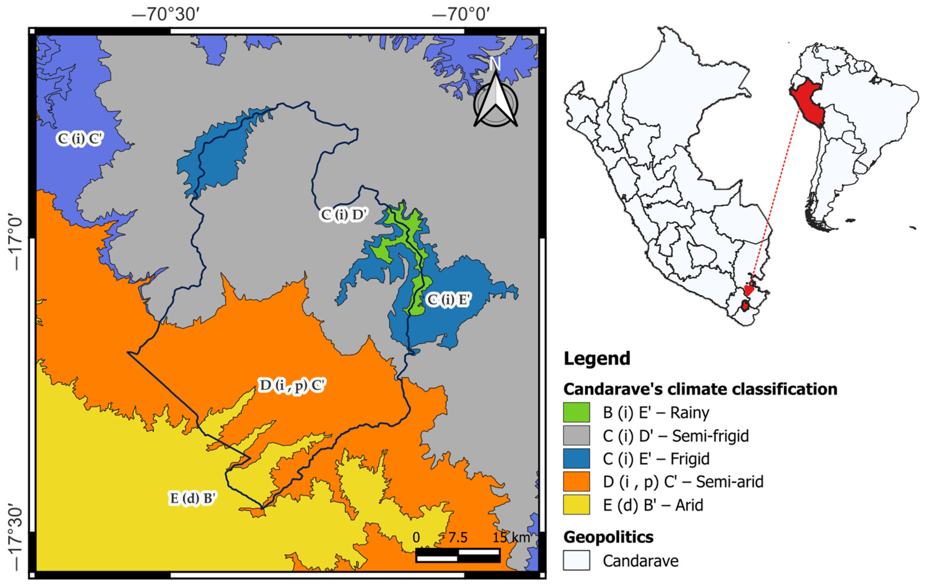
2.1. Study Area

The Province of Candarave is located in the northeastern corner of the Tacna Region, between the geographic coordinates 16°17′04″ S and 17°27′56″ S latitude, and 70°03′32″ W and 70°34′52″ W longitude. Its altitude varies from 2400 to 5500 m.a.s.l.

Most of the study area has a semi-arid climate with a dry winter and spring (between 50 mm and 120 mm annual rainfall), and a semi-frigid climate with a dry winter (between 500 mm and 700 mm annual rainfall) (Figure 1). Figure 2 shows the average monthly rainfall and maximum and minimum temperature in one of the weather stations inside the semi-arid area.

According to a report about drought regionalization in Perú using the SPI [19], there are eight homogeneous regions with particular characteristics regarding the occurrence of droughts. These regions are distributed spatially across the country’s three hydrographic basins (Figure 3). Based on Figure 3, the study area belongs to the fifth region, CS, which covers the stations of the country’s southern coast in the Pacific Basin.

The methodology followed in this study is summarized in Figure 4.

2.2. Data Collection

To carry out this research, it was necessary to collect gridded-based and observed meteorological data, historical and future climate data, and satellite images. Processed data were used to calculate drought indicators. These indicators are the basis for characterizing droughts in the study area.

2.2.1. Gridded-Based Meteorological Data

This study used two gridded-based precipitation datasets generated for the Peruvian territory (

Table 1. Gridded-base precipitation datasets used in this study.

Product	Abbreviation	Version	Source	Resolution	Frequency	Period
Rain for Peru and Ecuador [24]	RAIN4PE	v.1.0	International Climate Initiative (IKI)	0.1° × 0.1°	Daily	1981–2015
Peruvian Interpolated Data of SENAMHI’s Climatological and Hydrological Observations [25]	PISCO	v.2.1	SENAMHI	0.1° × 0.1°	Daily	1981–2016

). These datasets were assessed regarding their correlation with the field observed data collected at the weather stations. Based on the correlation results, gridded precipitation datasets were used to fill in missing data and to determine indicators of precipitation spatial variation [23]. These datasets were also used to create virtual weather stations.

2.2.2. Meteorological Data

Meteorological data were collected from six weather stations operated by SENAMHI. The quality of the data obtained from the weather stations was assessed regarding consistency, homogeneity, and trends.

The assessed meteorological data were then used to calculate the standardized precipitation index (SPI) and the standardized precipitation–evapotranspiration index (SPEI) from 1981 to 2015. Additionally, observed meteorological data were used to adjust gridded datasets, both weather-gridded data (the basis for virtual weather station creation) and climate-gridded data (the basis for climate change assessment).

Table 2. Weather stations used in this study.

Weather Station Name	Province	Geographic Coordinates (Degrees)		Altitude (m.a.s.l.)	Variable
		Longitude	Latitude
Aricota	Candarave	−70.2354	−17.3256	2850	Rainfall and temperature
Cairani	Candarave	−70.3667	−17.2833	3443	Rainfall and temperature
Candarave	Candarave	−70.2673	−17.2906	3415	Rainfall and temperature
Carumas	Mariscal Nieto	−70.6944	−16.8131	2976	Rainfall
Titijones	Mariscal Nieto	−70.5260	−16.6179	4609	Rainfall
Vilacota	Tarata	−70.0503	−17.1169	4438	Rainfall

shows information about the six weather stations.

2.2.3. Virtual Weather Stations

Creating virtual weather stations to perform a spatial drought analysis was necessary due to insufficient actual weather stations inside and near the study area (Figure 1). Many of the most popular interpolation methods are unsuitable for this study due to the sparse point distribution and the lack of stations in the area. Altitude could also play a significant role, as it changes rapidly in the study region.

The following steps were taken to generate virtual weather stations:

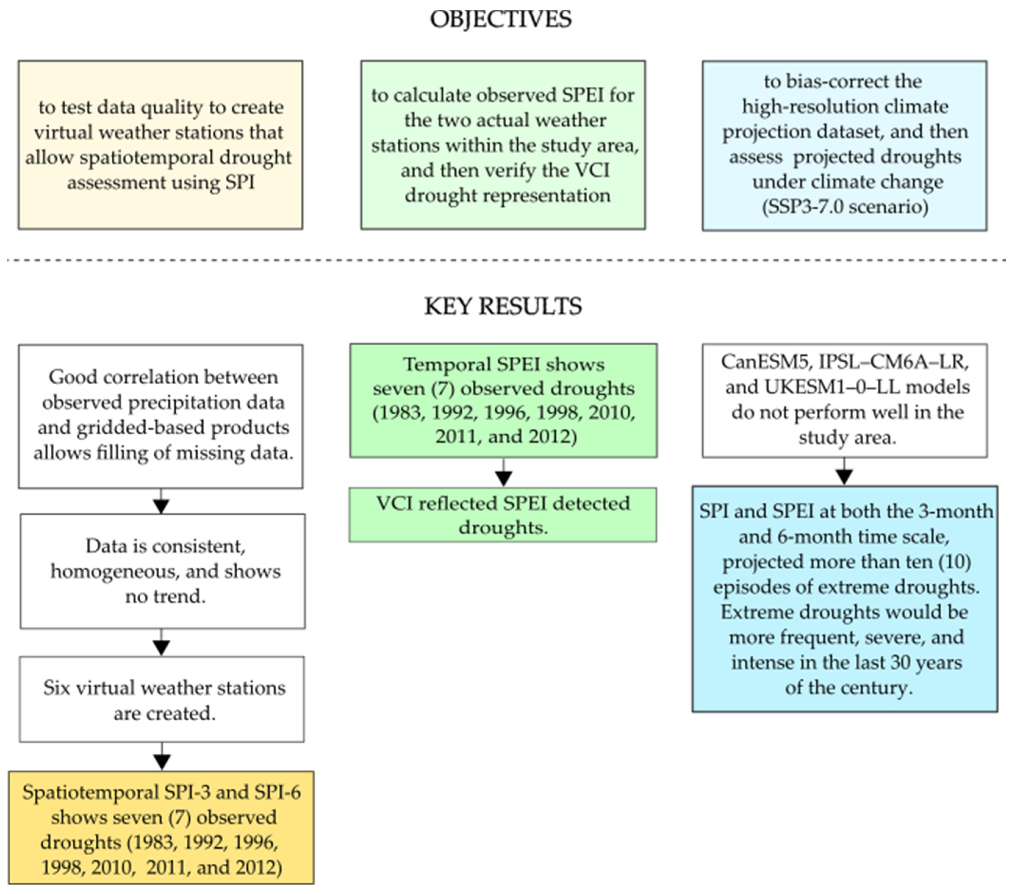
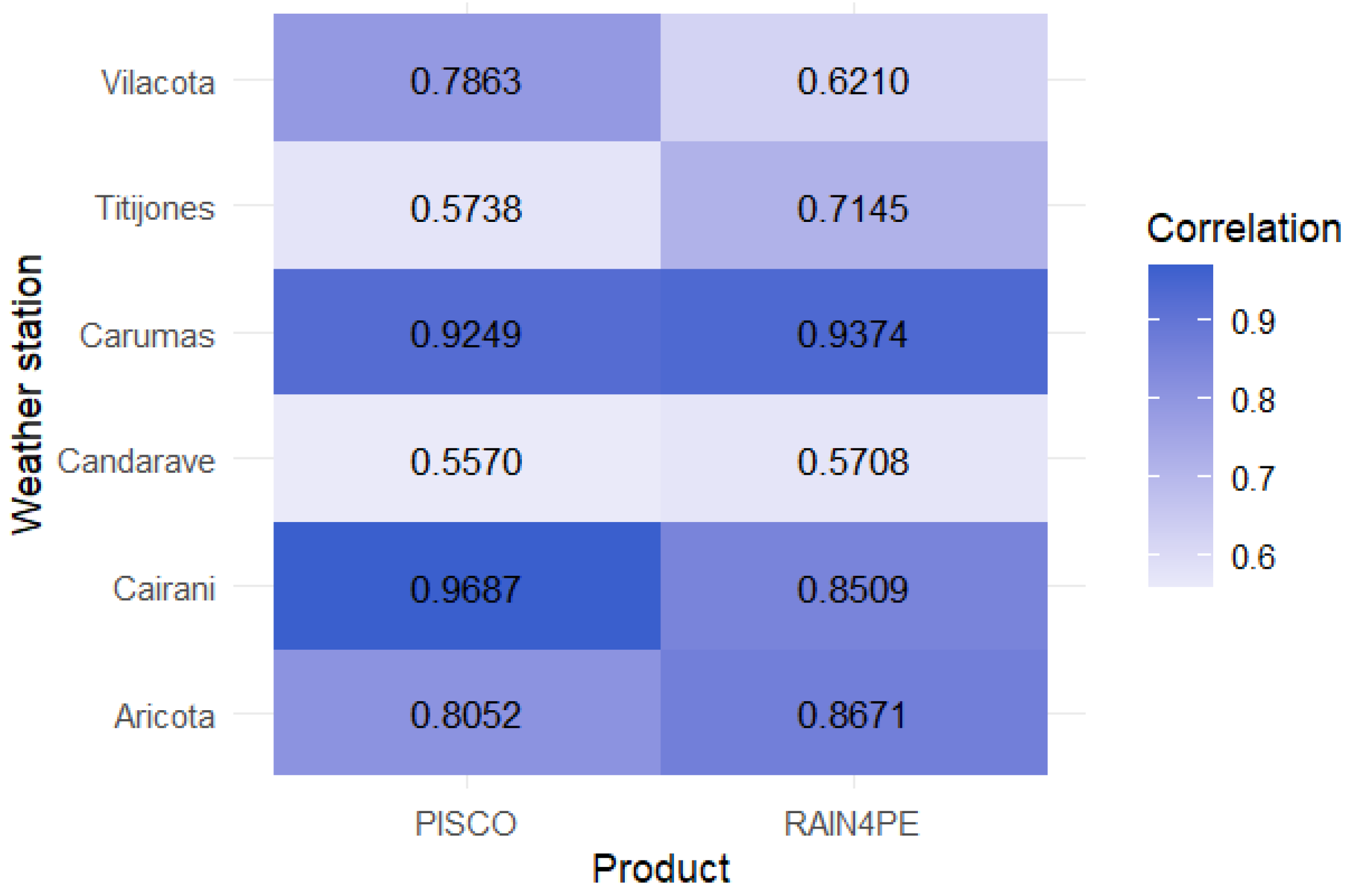
• Performing correlation between gridded-based meteorological data (PISCO and RAIN4PE datasets) and data from actual weather stations. According to these results, the adequate dataset was used to extract data from the location of the proposed virtual weather station;
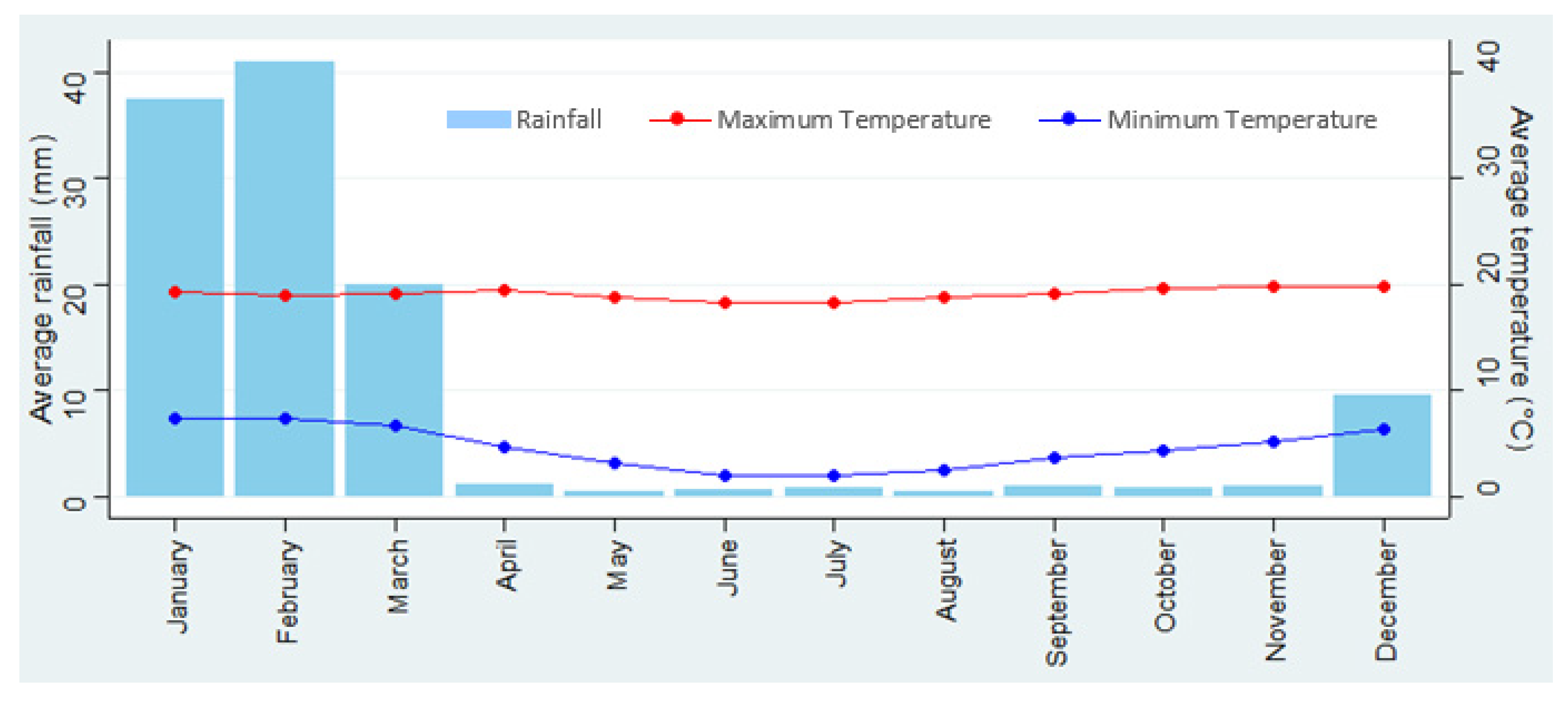
• Assessment of rainfall features; for this purpose, the sum of the average rainfall of the months where the wet season occurs (December to March) was evaluated. This sum was compared among the weather stations;
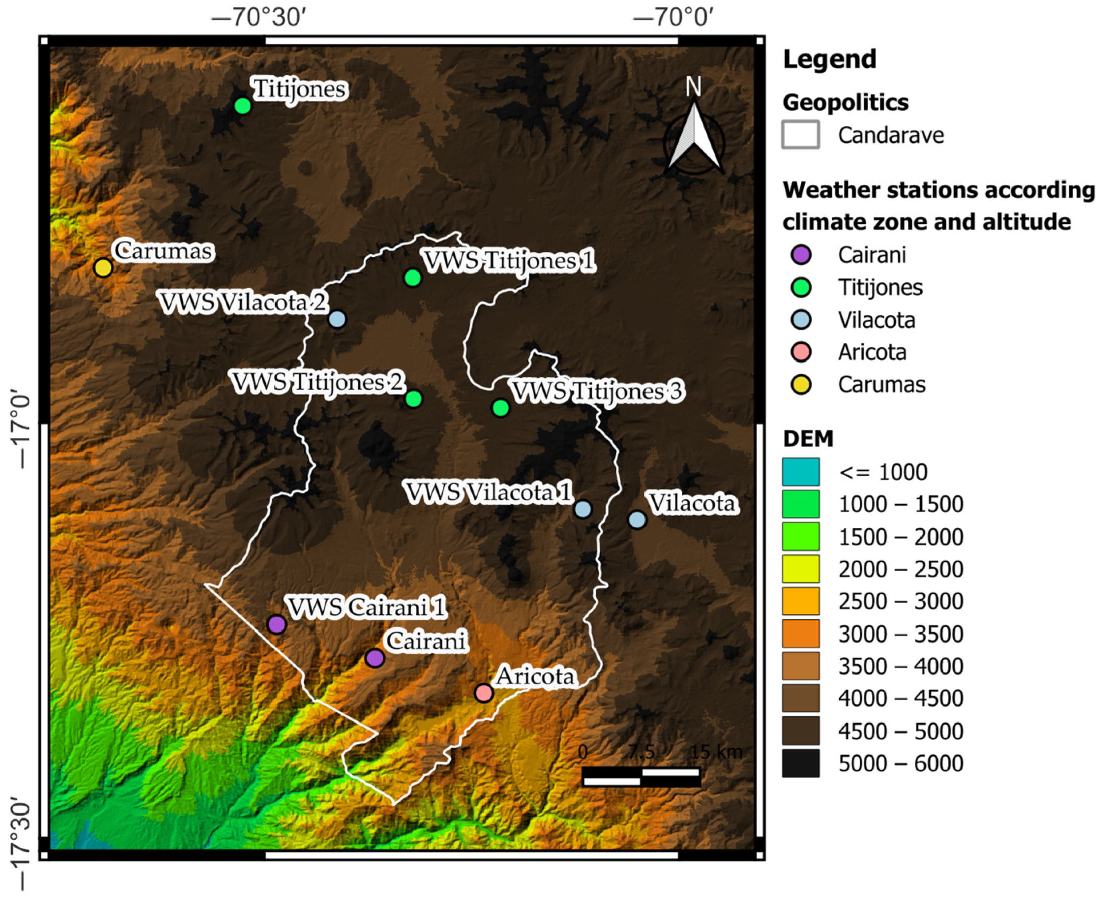
• Setting the location of the virtual weather stations according to their climatic zones and altitudes (Figure 5). Virtual weather stations are located within the same climatic zones as the actual weather station having considered a similar altitude as well;
• The gridded-based data for the virtual station location were corrected using the same linear correlation model found in Step 1 for each actual weather station.

Table 3. Features of the created virtual weather stations.

Virtual Weather Station Name	Climate	Geographic Coordinates (Degrees)		Altitude (m.a.s.l.)
		Longitude	Latitude
Titijones	Semi-frigid	−70.5260	−16.6179	4609
VWS Titijones 1	Semi-frigid	−70.321	−16.825	4646
VWS Titijones 2	Semi-frigid	−70.320	−16.971	4667
VWS Titijones 3	Semi-frigid	−70.215	−16.982	4594
Vilacota	Frigid	−70.0503	−17.1169	4438
VWS Vilacota 1	Frigid	−70.116	−17.104	4556
VWS Vilacota 2	Frigid	−70.412	−16.875	4558
Cairani	Semi-arid	−70.3667	−17.2833	3443
VWS Cairani 1	Semi-arid	−70.485	−17.243	3486

shows the location and other features of the created virtual weather stations. These virtual weather stations only contain rainfall information due to the lack of temperature data in the actual weather stations and their very low correlation with gridded-based products like PISCO.

2.2.4. Climate Data

To project local drought conditions in the study area during 2015–2100, a high-resolution climate projection dataset based on the CMIP6 for Peru (BASD-CMIP6-PE) was used. This dataset has a 1-day and 10 km resolution, and it is based on the bias-adjusted and statistically downscaled CMIP6 climate projections of 10 GCMs (

Table 4. Bias-adjusted and statistically downscaled CMIP6 models used in this study.

No.	Model	Member
1	CanESM5	r1i1p1f1
2	IPSL–CM6A–LR	r1i1p1f1
3	UKESM1–0–LL	r1i1p1f1
4	CNRM–CM6–1	r1i1p1f1
5	CNRM–ESM2–1	r1i1p1f1
6	MIROC6	r1i1p1f1
7	GFDL–ESM4	r1i1p1f1
8	MRI–ESM2–0	r1i1p1f1
9	MPI–ESM1–2–HR	r1i1p1f1
10	EC–Earth3	r1i1p1f1

Source: [26].

) under three Shared Socioeconomic Pathways (SSP1-2.6, SSP3-7.0, and SSP5-8.5) [26].

The BASD-CMIP6-PE dataset is available at https://www.pik-potsdam.de/data/doi10.5880PIK.2023.001/ accessed and downloaded on 19 August 2024.

This research focused on SSP3-7.0, where SSP3 represents a fragmented world with limited global cooperation, focusing on regional challenges, and 7.0 indicates a high greenhouse gas emissions pathway [27]. This scenario envisions significant challenges to mitigation and adaptation efforts due to socio-economic inequalities and environmental degradation.

2.2.5. Satellite Data

Landsat satellite data were acquired to calculate the Normalized Difference Vegetation Index (NDVI). The Google Earth Engine platform was used to process Landsat 5 and 8 satellite images, considering some requirements such as choosing images with a cloud cover percentage of less than 11% [28] (

Table 5. Downloaded scenes, Landsat Collections, (https://developers.google.com/earth-engine/datasets/catalog/landsat accessed on 9 September 2024), and period.

Data	Year	Product Identifier	Sensing Time (hh:mm:ss)	Cloud Cover %	Patch/Row
Landsat 5	1990	LANDSAT/LT05/C02/T1_L2/LT05_002072_19900222	14:12:54	4	02/72
		LANDSAT/LT05/C02/T1_L2/LT05_002072_19900513	14:01:54	2
		LANDSAT/LT05/C02/T1_L2/LT05_002072_19900614	14:01:47	0
Landsat 5	1992	LANDSAT/LT05/C02/T1_L2/LT05_002072_19920127	14:05:58	0	02/72
		LANDSAT/LT05/C02/T1_L2/LT05_002072_19920502	14:05:27	0
		LANDSAT/LT05/C02/T1_L2/LT05_002072_19920705	14:04:46	1
		LANDSAT/LT05/C02/T1_L2/LT05_002072_19920907	14:03:51	1
Landsat 5	1996	LANDSAT/LT05/C02/T1_L2/LT05_002072_19960513	13:52:38	0	02/72
		LANDSAT/LT05/C02/T1_L2/LT05_002072_19960801	13:56:57	1
		LANDSAT/LT05/C02/T1_L2/LT05_002072_19961004	14:00:24	9
		LANDSAT/LT05/C02/T1_L2/LT05_002072_19961121	14:02:43	0
Landsat 5	1998	LANDSAT/LT05/C02/T1_L2/LT05_002072_19980519	14:19:08	0	02/72
Landsat 5	2010	LANDSAT/LT05/C02/T1_L2/LT05_002072_20101112	14:31:25	3.2	02/72
		LANDSAT/LT05/C02/T1_L2/LT05_002072_20101214	14:31:29	3
Landsat 5	2011	LANDSAT/LT05/C02/T1_L2/LT05_002072_20110726	14:30:40	9	02/72
		LANDSAT/LT05/C02/T1_L2/LT05_002072_20111115	14:29:05	7
Landsat 8	2015	LANDSAT/LC08/C02/T1_L2/LC08_002072_20150502	14:40:50	5.17	02/72
		LANDSAT/LC08/C02/T1_L2/LC08_002072_20151126	14:41:48	10.51
Landsat 8	2016	LANDSAT/LC08/C02/T1_L2/LC08_002072_20160504	14:41:15	6.51	02/72
		LANDSAT/LC08/C02/T1_L2/LC08_002072_20160723	14:41:38	0.4
		LANDSAT/LC08/C02/T1_L2/LC08_002072_20161128	14:41:58	4.97
Landsat 8	2020	LANDSAT/LC08/C02/T1_L2/LC08_002072_20201123	14:41:58	3.51	02/72
Landsat 8	2021	LANDSAT/LC08/C02/T1_L2/LC08_002072_20210502	14:41:10	0.11	02/72
		LANDSAT/LC08/C02/T1_L2/LC08_002072_20210721	14:41:36	0.14
		LANDSAT/LC08/C02/T1_L2/LC08_002072_20210822	14:41:49	1.47
		LANDSAT/LC08/C02/T1_L2/LC08_002072_20211110	14:42:01	3.08
Landsat 8	2022	LANDSAT/LC08/C02/T1_L2/LC08_002072_20220606	14:41:43	2.76	02/72
		LANDSAT/LC08/C02/T1_L2/LC08_002072_20220825	14:42:11	0.54

).

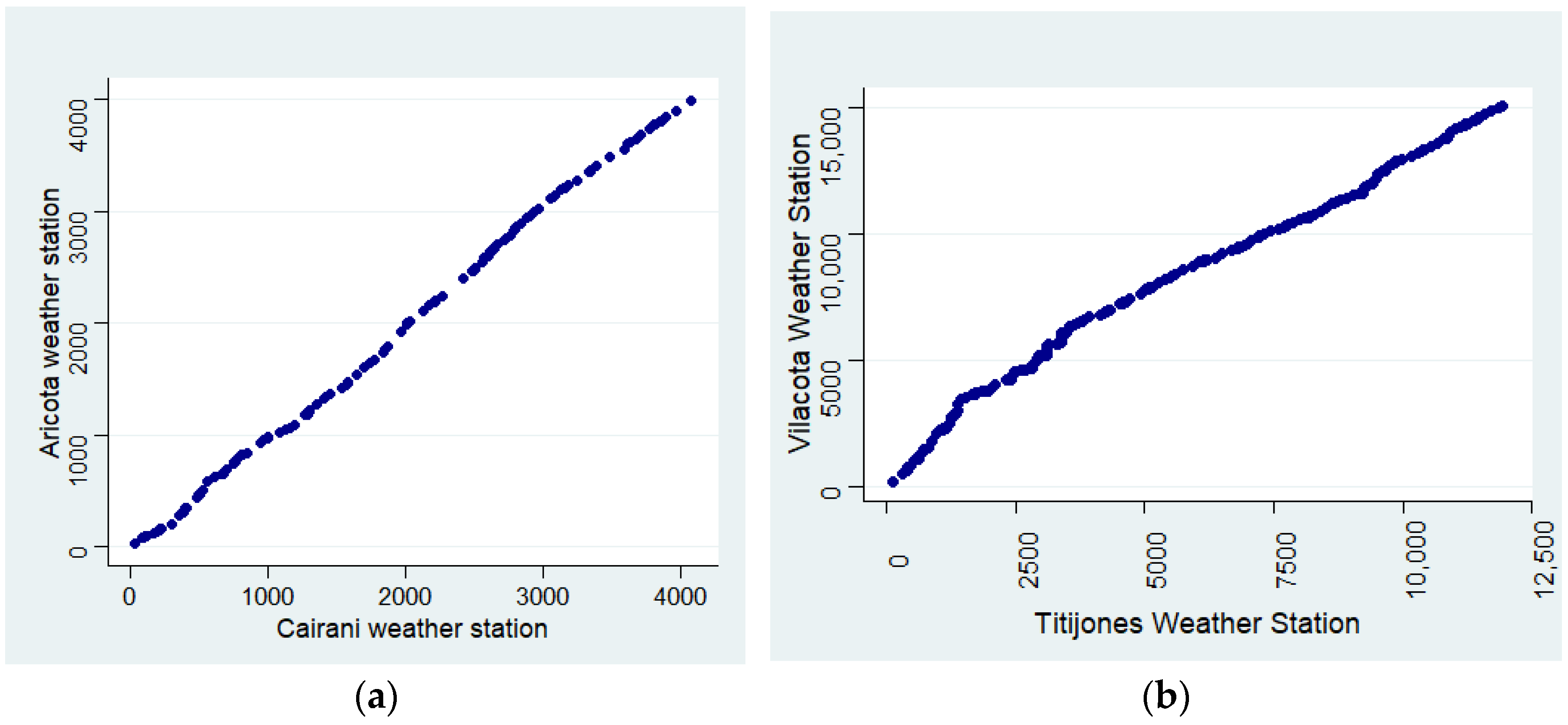
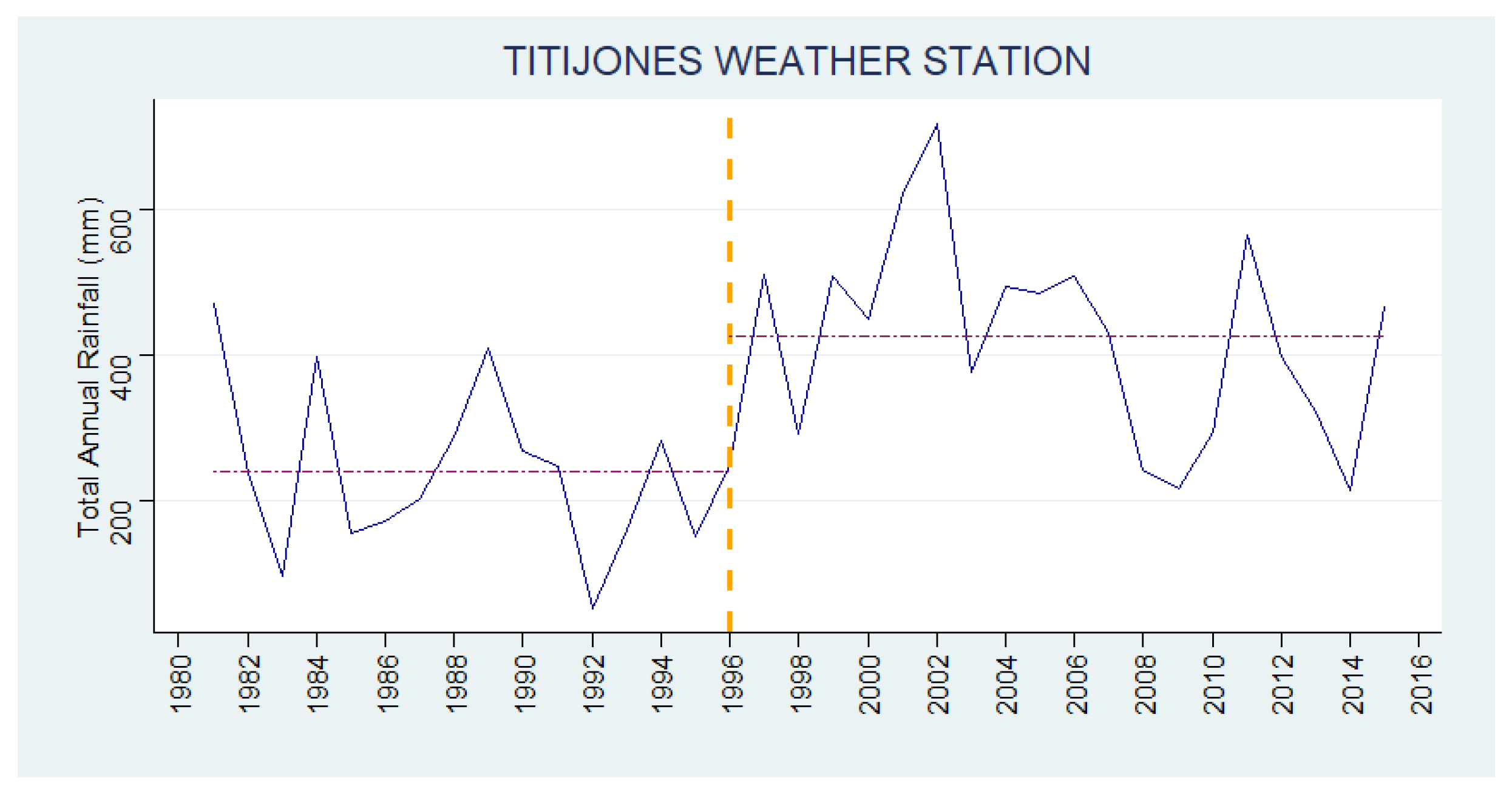
2.3. Data Quality Control

Before creating the virtual weather stations and after filling in the missing data, the quality of the observed meteorological data was assessed regarding its consistency, homogeneity, and trends. For this purpose, total annual rainfall data were used.

The double-mass curve test is used to verify data consistency by comparing data for one station with that of a pattern composed of the data from several other stations nearby [29,30], Also, homogeneity tests were performed as an annual series, and then, they were adjusted in case needed. The homogeneity tests applied in this study are shown in Table S1. Finally, the Mann–Kendall trend test is used to determine the presence of a monotonic trend in a time series [31].

On the other hand, bias correction and model performance were developed to secure a good local representation of the climate data. Even though the BASD-CMIP6-PE dataset was developed for Peru and is already downscaled, it still needs bias correction for a local scale. Quantile mapping (QM) is one of the most popular bias correction methods. This method corrects the cumulative distribution function (CDF) of the predicted value from the CDF of the observed value [32]. Additionally, many parametric or non-parametric correction methods originated on this principle, such as distribution-derived transformations, parametric transformations, and empirical quantiles [32]. In this study, non-parametric quantile mapping using the empirical quantiles method performed better on the correction of the meteorological variables. This method uses the empirical distribution of the data without fitting it to any theoretical distribution. The R package, qmap v. 1.0-4, was used to apply the quantile mapping methods.

Furthermore, after bias correction, the performance of each model was assessed using the Taylor Diagram [33] and the percentage bias (Equation (1)).

$$\mathrm{P}\mathrm{B}\mathrm{I}\mathrm{A}\mathrm{S}={\displaystyle \frac{{\sum }_{i=1}^n(M_i-O_i)}{{\sum }_{i=1}^n{O}_i}}$$

(1)

where n is the number of observations under evaluation, and M and O are the modeled and observed data. The optimal value of PBIAS is zero, and it moves away from being satisfactory as the values tend toward both directions (–∞ and +∞). Positive PBIAS values indicate a model underestimation bias.

The performance of the models was evaluated individually using the Taylor diagram. The Taylor diagram also takes into account the spatial correlation coefficient (CC), the centered root mean square error (RMSE), and the normalized standard deviation ratio (σ) of the modeled and observed data, which are commonly used to assess the agreement between simulated and observed data [33].

After the model performance assessment, monthly climate model output data for precipitation, and minimum and maximum temperature, were obtained from the BASD-CMIP6-PE multi-model ensemble (MME). Many researchers have concluded that MME performs better than individual models by reducing the simulation uncertainty [13,34]. In this study, the methodology stated by Lei et al. [34] was followed to ensemble the models using a weighted scheme. Summarizing, the rank of the individual model at each meteorological variable is calculated using four metrics (CC, RMSE, RB, and σ), and then these ranks are normalized, summing one. The mean of the four metrics is the model’s weight; therefore, the sum of the weights is also one.

2.4. Drought Indicators

This study uses 3-month and 6-month SPI and SPEI time scales. The 3-month time scale was selected as a short-term scale that reflects moisture conditions, and the 6-month time scale was chosen as a medium-term scale that reflects trends in precipitation [35].

SPI and SPEI from 1981 to 2015 were used to analyze observed extreme drought, and SPI and SPEI from 2016 to 2100 were used to assess projected extreme droughts.

2.4.1. Standardized Precipitation Index (SPI)

SPI is a widely used tool for assessing drought conditions by quantifying precipitation deviations over a specific period [36]. Its main advantage is that it relies solely on precipitation data, which are often readily available, making it a cost-effective and convenient tool, particularly in regions with limited or unreliable meteorological data such as temperature and evapotranspiration [37]. The SPI can be applied across various temporal and spatial scales due to its flexible and standardized nature. This enables the characterization of multiple types of drought events, from short-term droughts to prolonged droughts, and from meteorological to hydrological drought [38,39].

A drought is considered when SPI is less than −1 and ends when SPI becomes positive (

Table 6. Classification of drought conditions according to SPI.

SPI Value	Classification
−2.0 and less	Extreme drought
−1.5 to −1.99	Severe drought
−1.0 to −1.49	Moderate drought
−0.99 to 0.99	Normal conditions

). Its magnitude is measured by summing the indicator values over a drought period [40].

The SPI is calculated by fitting a probability density function to the rainfall frequency distribution as a sum outside the interval of interest. This process is performed separately for each month or timescale of the rainfall data time series and for each location in the interval. Then, each probability density function is transformed into a standard normal distribution. According to [41], climatic precipitation data follow a gamma distribution, one of the most frequently occurring distributions in technical hydrology. It is a positively skewed distribution defined only for the positive values of the variable, as summarized in Table S2 based on [42].

In this study, SPI was obtained using the SPI Generator Software v. 1.7.5. [43].

2.4.2. Standardized Precipitation Evapotranspiration Index (SPEI)

Vicente-Serrano [44] proposed SPEI based on the SPI and the water balance principle. SPEI uses the difference between precipitation (P) and potential evapotranspiration (PET) as an input condition to assess dry and wet conditions in the area. The climate–water balance is calculated using Equation (2).

$$D_i=P_i-{PET}_i$$

(2)

where D_i is the moisture deficit (mm) in month i, P_i is the precipitation (mm) in month i, and PET_i is the potential evapotranspiration (mm) in month i. According to [3], PET is estimated using the Penman–Monteith method or the Hargreaves method.

The values of D_i are summarized over different time scales in Equation (3).

$$D_n^k={\sum }_{i=0}^{k=1}\left(P_{n-\mathrm{i}}-{PET}_{n-1}\right), n\ge k$$

(3)

where k is the monthly time scale and n is the number of calculations.

A three-parameter log-logistic probability density function was used to adjust the established data series (Equation (4)).

$$f\left(x\right)={\displaystyle \frac{\beta }{\alpha }}{({\displaystyle \frac{x-\mathsf{\gamma }}{\alpha }})}^{\beta -1}{[1+{({\displaystyle \frac{x-\mathsf{\gamma }}{\alpha }})}^{\beta }]}^{-2}$$

(4)

where α, β, and γ are scale, shape, and origin parameters, respectively.

Thus, the cumulative distribution function for a given time scale was defined by Equation (5).

$$F\left(x\right)={[1+{({\displaystyle \frac{\alpha }{x}}-\gamma )}^{\beta }]}^{-1}$$

(5)

SPEI is calculated using Equation (6), as the standardized values of F(x).

$$SPEI=W-{\displaystyle \frac{C_0+C_{1}W+C_2{W}^2}{1+d_{1}W+d_2{W}^2+d_3{W}^3}}$$

(6)

where:

$$W=\sqrt{-2\ln \left(P\right)} for P\le 0.5$$

P is the probability of exceeding a given D value, $P=1-F\left(x\right)$.

If P > 0.5, then p is replaced by 1 − P and the sign of the resultant SPEI is reversed.

$$C_0=2.515517, C_1=0.802853, C_2=0.010328$$

$$d_1=1.432788, d_2=0.189269, d_3=0.001308$$

This means that negative values indicate drier conditions than average, while positive values indicate wetter conditions than average. The drought categories are shown in

Table 7. Classification of drought conditions according to SPEI.

SPEI Value	Classification
−2.0 and less	Extreme drought
−1.5 to −1.99	Severe drought
−1.0 to −1.49	Moderate drought
−0.99 to 0.99	Normal conditions

.

2.4.3. Vegetation Condition Index (VCI)

The Vegetation Condition Index (VCI) is a tool used to assess the health and vitality of vegetation in a specific region [45]. This index is calculated by measuring the reflectance of vegetation in different spectral bands, such as near-infrared (NIR) and red, using satellite images or ground sensors [46]. The VCI is based on the principle that healthy vegetation reflects light differently in these spectral bands compared to non-vegetated areas or stressed vegetation.

A commonly used vegetation index known as the Normalized Difference Vegetation Index (NDVI) is utilized to calculate VCI. The NDVI is calculated using Equation (7).

NDVI = (NIR − Red)/(NIR + Red)

(7)

NIR is the reflectance in the near-infrared band, and Red is the reflectance in the red band.

The interpretation of NDVI indicates that higher values are associated with greater vegetation cover and better vegetative health, while lower values suggest less vegetation or stressed vegetation. The VCI uses NDVI as a foundation and often involves comparing NDVI values over time to assess trends in vegetation conditions [47]. This is particularly useful for monitoring crops, managing natural resources, and evaluating ecosystem health.

Equation (8) is used to obtain VCI.

$$VCI= {\displaystyle \frac{{NDVI}_i-{NDVI}_{min}}{{NDVI}_{max}-{NDVI}_{min}}}\times 100$$

(8)

A lower VCI indicates a condition of drought and stress in vegetation (

Table 8. VCI ranges and their classification.

VCI Ranges (%)	Classification
0 < VCI < 20	Extremely dry
20 ≤ VCI < 40	Dry
40 ≤ VCI < 60	Normal condition
60 ≤ VCI < 80	Good condition
VCI ≥ 80	Optimal condition

Source: [17].

).

3. Results and Discussion

Figure 6 shows the key findings of this study according to the objectives.

3.1. Data Quality

3.1.1. Gridded-Based Meteorological Data

Figure 7 shows the correlation between the two gridded datasets used in this study and observed precipitation data from weather stations. As all correlation values are higher than 0.5, the gridded products performed moderately to very well in the study area. However, the Candarave Weather Station is no longer used in this study due to its low correlation with both gridded products and neighboring weather stations (Cairani and Aricota). The other weather stations were utilized to fill in missing observed data.

3.1.2. Meteorological Data

A total annual rainfall series was obtained after the completion of daily rainfall data using the better correlation gridded dataset (Table S3).

Figure 8 shows the double-mass curves for the weather stations with similar altitudes; while Aricota and Cairani show good consistency in their data, Titijones and Carumas show some smooth slope changes.

Additionally, homogeneity tests to detect changing points (steps) in the time series, as well as trend analysis, were performed (

Table 9. Homogeneity and trend test results.

Test 1	Results	Aricota	Cairani	Carumas	Titijones	Vilacota
Standard Normal Homogeneity Test (SNHT)	Test statistic	3.1772	4.8296	5.7184	12.237	5.5791
	p-value	0.6028	0.2958	0.1927	0.00385	0.2069
	Result	Homogeneous	Homogeneous	Homogeneous	Not homogeneous	Homogeneous
	Probable change point	–	–	–	1996	–
Buishand Range Test	Test statistic	1.1614	0.90446	1.1952	1.8814	1.287
	p-value	0.3363	0.744	0.3007	0.00165	0.2026
	Result	Homogeneous	Homogeneous	Homogeneous	Not homogeneous	Homogeneous
	Probable change point	–	–	–	1996	–
Pettitt’s test for single change-point detection	Test statistic	98	80	144	216	102
	p-value	0.5414	0.8373	0.1191	0.003501	0.4856
	Result	Homogeneous	Homogeneous	Homogeneous	Not homogeneous	Homogeneous
	Probable change point	–	–	–	1996	–
Mann–Kendall trend test	Test statistic	0.34083	−0.45445	0.73847	−0.6248 2	1.7042
	p-value	0.7332	0.6495	0.4602	0.5321	0.08835
	Result	No trends	No trends	No trends	No trends	No trends

¹ All tests were performed for n = 35. ² The test was performed after time series adjustment.

).

As can be seen in Table 9 and Figure 9, the rainfall data corresponding to Titijones Weather Station show a discontinuity due to a changing point in 1996. The methodology stated by [48] was followed to adjust the rainfall time series in Titijones. The values before the changing point were multiplied by a factor A calculated according to Equation (9).

$$\mathrm{A}={\displaystyle \frac{{\mathrm{q}}_{\mathrm{a}}}{{\mathrm{q}}_{\mathrm{b}}}}$$

(9)

where q_a and q_b are the means of {q_i} after and before the changing point date.

Figure 10 shows the adjusted rainfall data series in Titijones with no changing point presence.

On the other hand, according to the Mann–Kendall test for trend detection, data from all the stations show no autocorrelation and are identically distributed (Table 9).

3.1.3. Climate Data

Once the bias correction was performed on each model, the PBIAS was calculated to evaluate how well the corrected model represents the observed data. This was performed for both the precipitation data at 11 stations (Table S4) and the temperature data at 2 stations (Table S5). Only models with PBIAS values greater than −10 and less than 10 were considered for the subsequent analysis.

Regarding precipitation data, PBIAS indicated that CanESM5, IPSL–CM6A–LR, and UKESM1–0–LL models did not perform well for this study. Figure 11 confirms the PBIAS results as it can be seen that those models diverge from the solid black line that represents the statistics of the observed data.

Additionally, for maximum temperature, all the models showed good performance. However, for minimum temperature, most of the models performed moderately. In that case, only PBIAS values greater than −30 were considered. Like the precipitation variable, the CanESM5, IPSL–CM6A–LR, and UKESM1–0–LL models did not perform well in the area. Figure 12 and Figure 13 corroborate the performance results obtained with PBIAS.

As mentioned before, in this research, the methodology proposed by Lei et al. [34] was followed to calculate the performance of each model and thus obtain its weight in the MME. Tables S6 and S7 show the weights of each model for each station according to the studied variable. The data obtained from each model were then multiplied by the corresponding weight, resulting in projected meteorological variables up to 2100.

3.2. Drought Assessment

Three drought indexes were used to assess both historical and future droughts. SPI was utilized to study the spatiotemporal variability of the droughts. This was possible due to the creation of six virtual weather stations inside the study area. However, the virtual weather stations only provide rainfall data. Developing virtual weather stations with temperature variables was not possible due to the very low correlation between in-situ observed data and gridded-based products.

SPEI was calculated only in two locations inside the study area, Cairani and Aricota Weather Stations, because those data were available in the SENAMHI portal. SPEI was obtained, mainly to assess agricultural drought. Additionally, VCI use was evaluated to conduct the spatial analysis of agricultural droughts.

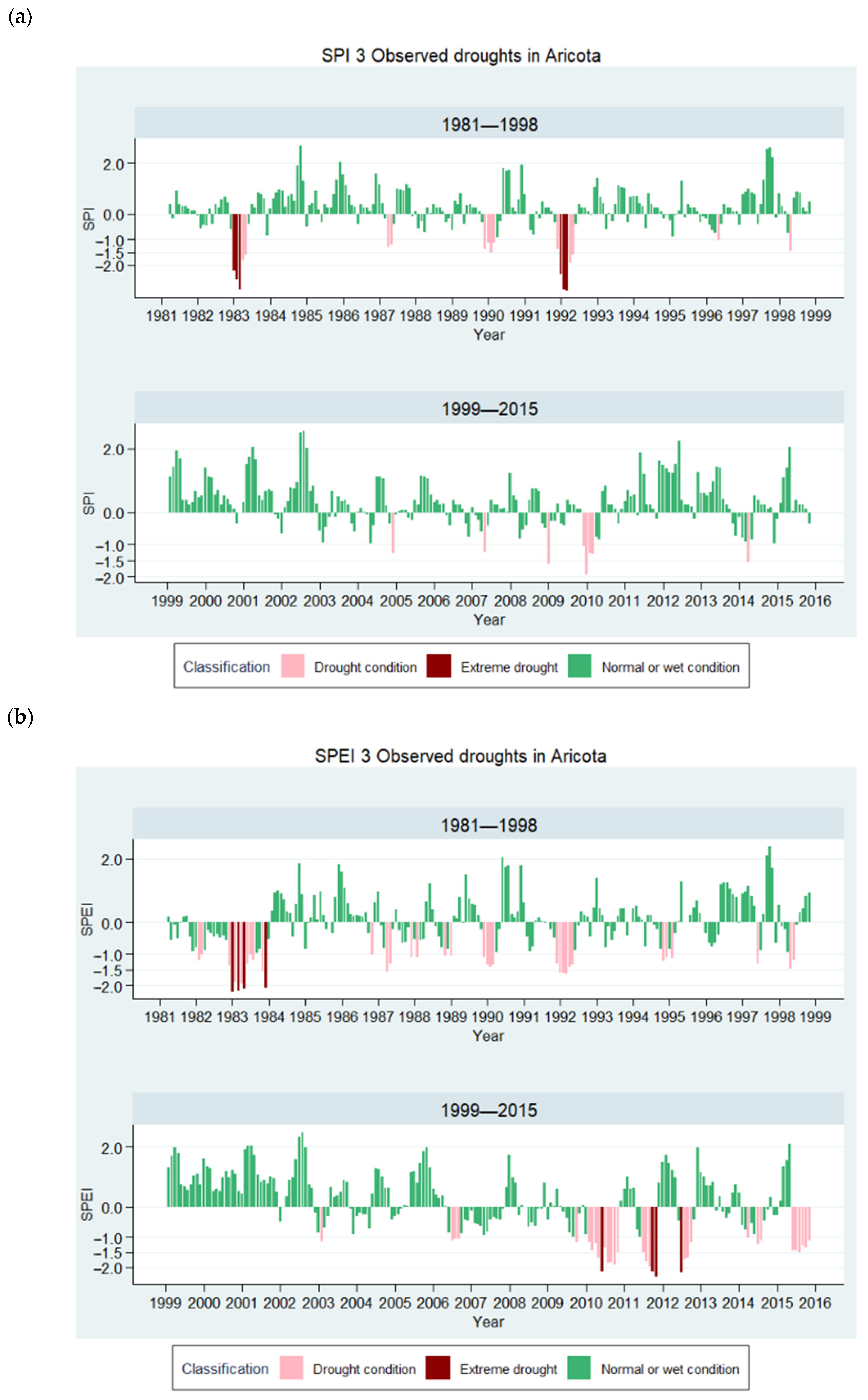
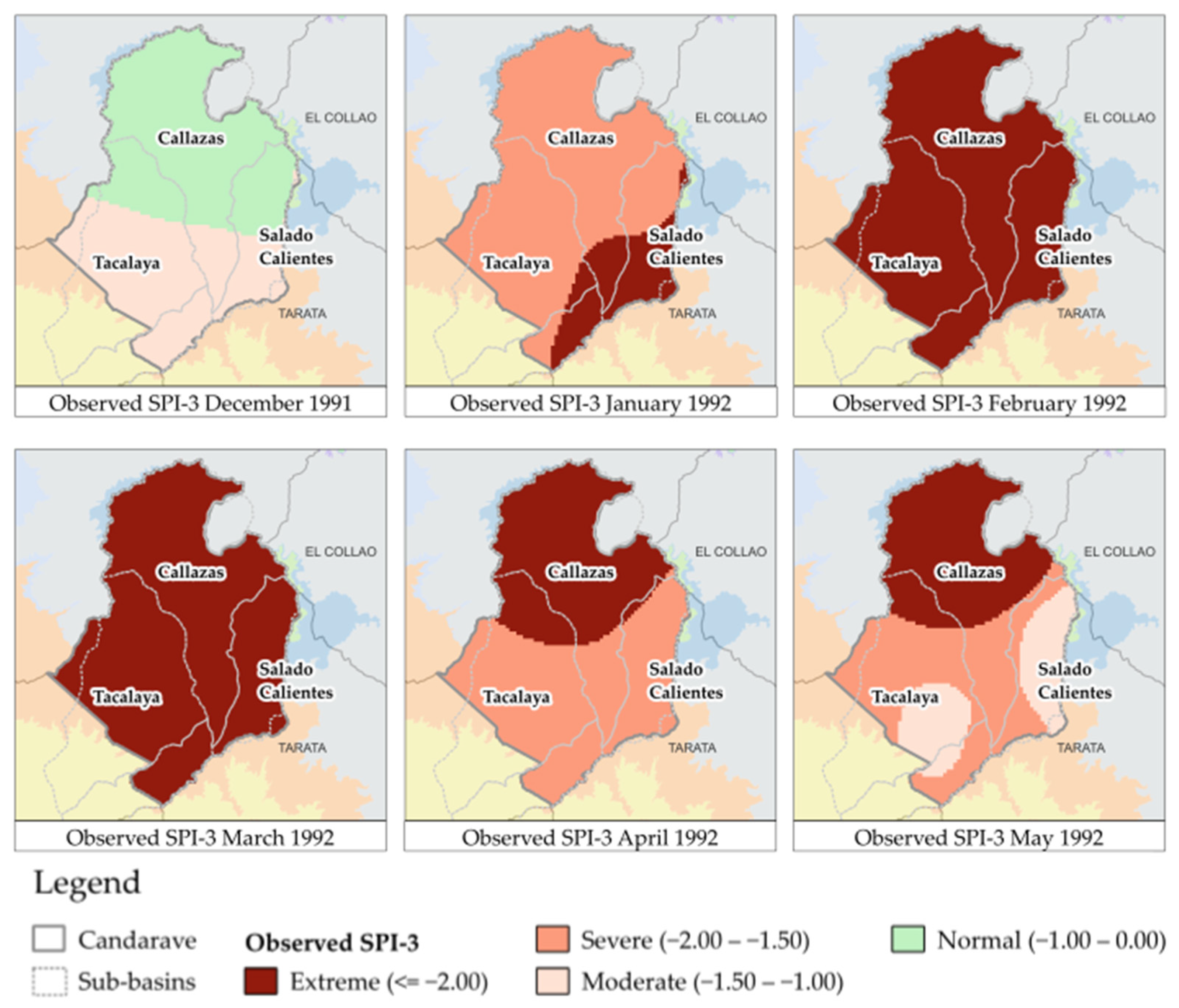
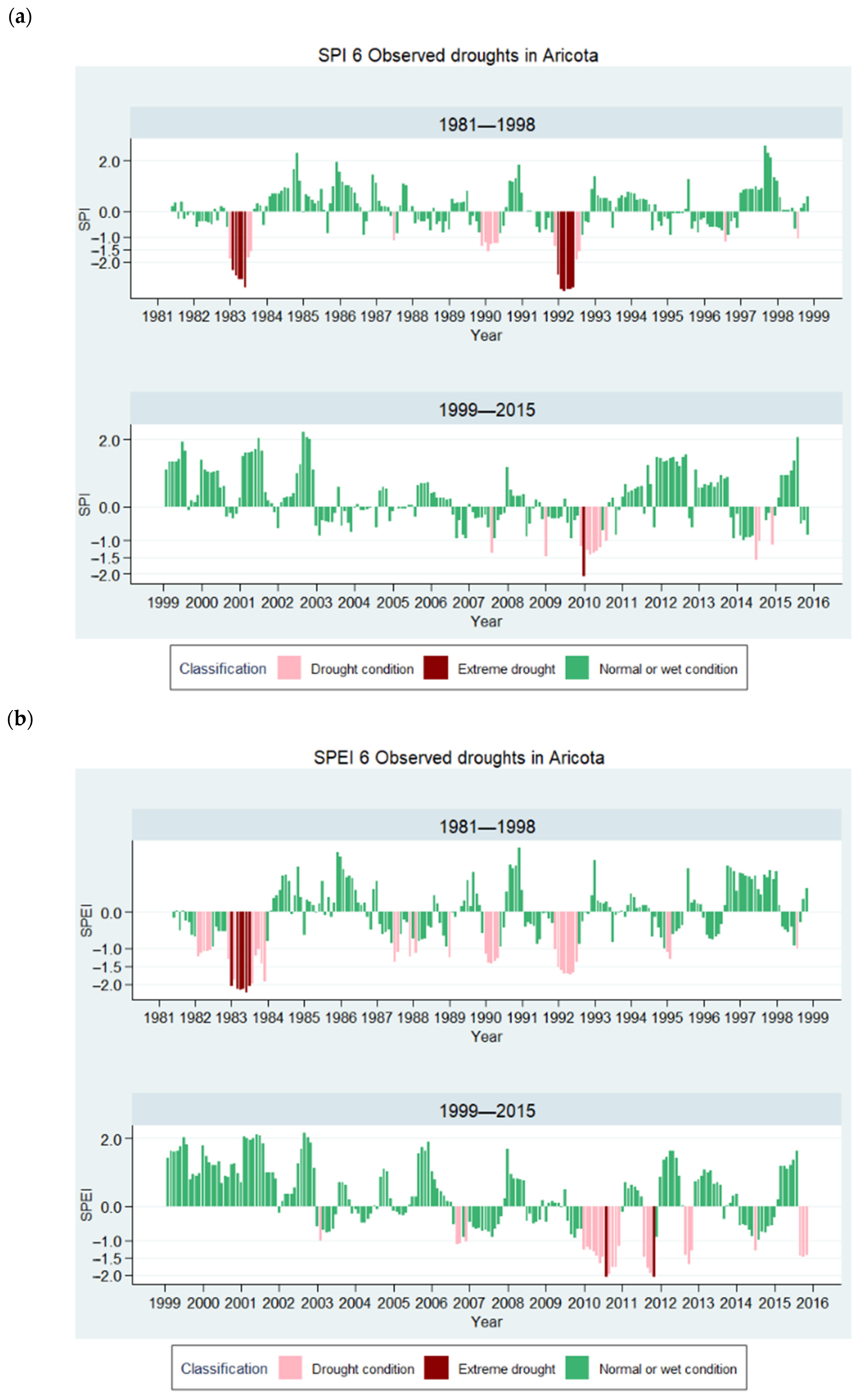
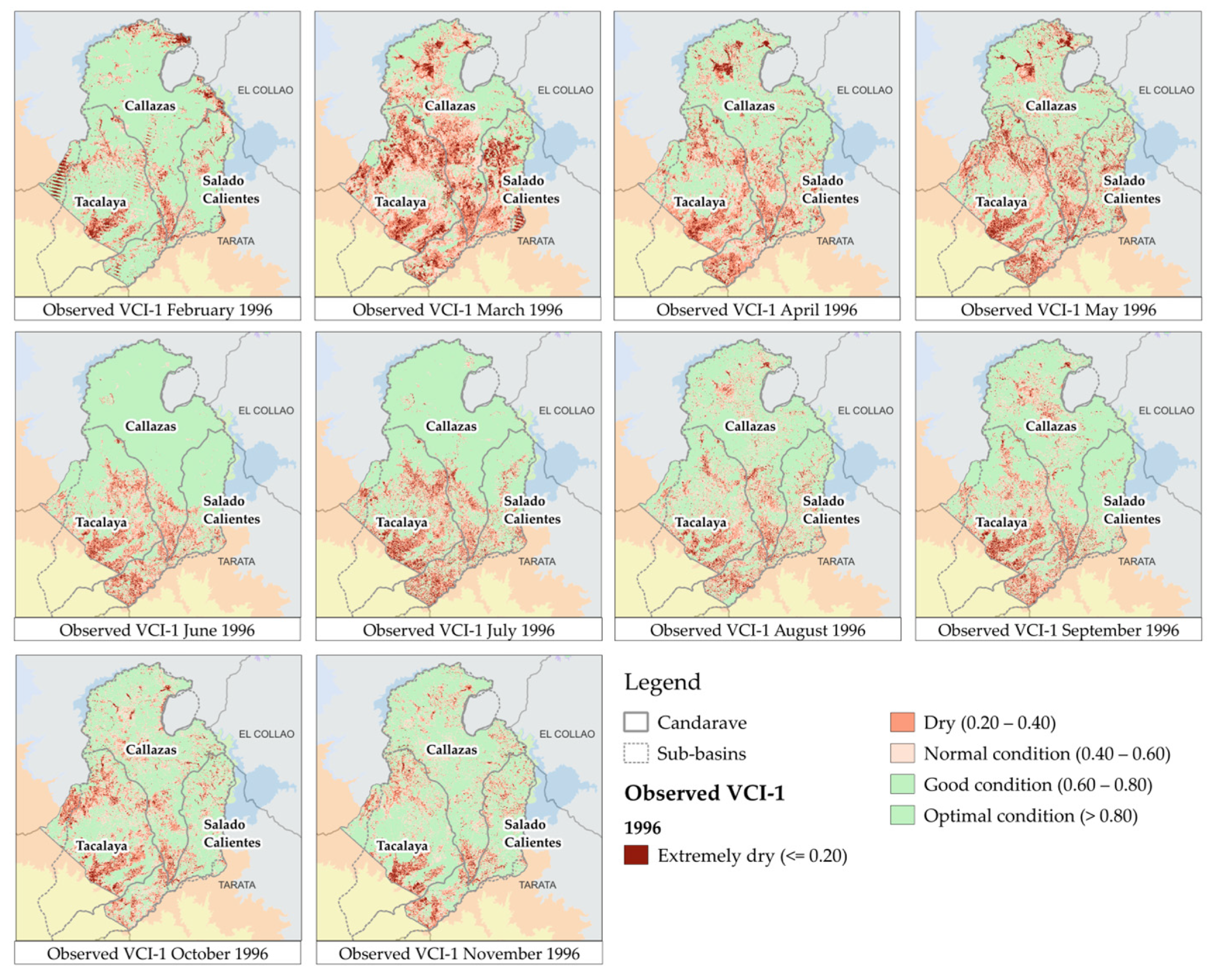
3.2.1. Observed Drought

Figure 14 shows the temporal variability of meteorological drought in the Aricota Weather Station.

SPI-3 noted extreme drought events in 1983 and 1992 (

Table 10. Observed drought features at a 3-month time scale according to SPI and SPEI results.

Index	Weather Station	Start Date	End Date	Duration (Months)	Maximum Intensity	Severity
SPI-3	Aricota	January 1983	June 1983	6	−2.97	−11.57
		January 1992	June 1992	6	−2.98	−12.21
	Cairani	February 1983	May 1983	4	−2.22	−6.90
		February 1992	May 1992	4	−3.04	−9.00
SPEI-3	Aricota	December 1982	January 1984	14	−2.18	−21.12
		February 2010	November 2010	10	−2.13	−16.08
		July 2011	November 2011	5	−2.32	−9.78
		July 2012	November 2012	5	−2.16	−−7.20
	Cairani	June 1995	December 1996	19	−2.15	−21.79
		December 1997	January 1999	14	−3.09	−19.29
		July 2012	November 2012	5	−2.67	−10.85

). This result is consistent with reports from SENAMHI that recognize the 1992 drought as the most severe, affecting a large part of the Peruvian territory [40]. There is no specific information about the impacts in the study area. However, at the national level, the drought had a significant effect on agriculture, resulting in economic losses of US$ 3.283 billion, or 11.6% of the annual Gross Domestic Product [40].

Nevertheless, while SPEI-3 did not report any drought in that year, it coincided with the extreme drought of 1983. SPEI might not have detected the 1992 drought due to an increase in precipitation occurring before a decrease in temperature [49]. Also, drought events at this small-time scale usually have short durations.

On the other hand, the virtual stations generated in this study allowed for spatial analysis of the droughts using SPI-3 (Figure 15). The most severe drought (1992) began to extend from the southern area of the province and gradually lost intensity in the same way.

Figure 16 shows the temporal variability of agricultural drought in the Aricota Weather Station. It is seen that SPEI drought events are less severe than the ones calculated with SPI because this one considers only precipitation data and it does not account for the mitigating effects of available moisture from the soil. Similar to the 3-month time scale, though SPEI did not detect the 1992 drought event as an extreme one, it coincided with the 1983 and the 2010 extreme drought events (

Table 11. Observed drought features at a 6-month time scale according to SPI and SPEI results.

Index	Weather Station	Start Date	End Date	Duration (Months)	Maximum Intensity	Severity
SPI-6	Aricota	February 1983	August 1983	7	−3.02	−16.72
		January 1992	November 1992	11	−3.14	−23.23
		January 2010	August 2010	8	−2.08	−10.42
	Cairani	March 1983	December 1983	9	−2.29	−11.42
		January 1992	November 1992	11	−3.14	−21.82
SPEI-6	Aricota	December 1982	January 1984	14	−2.15	−24.30
		January 2010	January 2011	13	−2.06	−18.51
		August 2011	December 2011	5	−2.06	−8.16
	Cairani	September 1995	December 1996	16	−2.19	−20.48
		March 1998	January 1999	11	−2.37	−16.70
		October 2012	November 2012	2	−2.20	−4.13

).

However, these results contrast with a study [50] which found that SPI was unable to identify severe droughts based on the short droughts in the area, although it could detect prolonged periodic drought episodes. This suggests that the performance of the indexes can vary by location, and there is no specific explanation for these variations yet. For instance, Chilean research concluded that warming trends are lower on the coast, so SPI could be a good indicator for coastal areas, while SPEI could be a good indicator for inland areas [51].

Due to the lack of weather stations in the study area and the low availability of temperature data, VCI was evaluated as an option to assess spatial agricultural droughts. Figure 17 shows the 1-month time scale VCI for the drought event detected by SPEI in 1996. It is seen that VCI detected vegetation affectation during the whole of 1996. Areas showing good condition correspond to bare soil or minimal vegetation. Even though, according to SPEI-6, the drought event started in September 1995, VCI shows more extremely dry areas in March 1996. That could be attributed to the biophysical changes that vegetation must undergo for the effect of drought to be detected by VCI [52]. Also, vegetation in semiarid regions may respond only to longer droughts because they are adapted to withstand frequent water deficits [52].

The usage of VCI for the study area should be studied more in detail because Landsat has many satellite images that do not meet the cloud cover requirements. This lack of information hinders VCI calculation at different time scales.

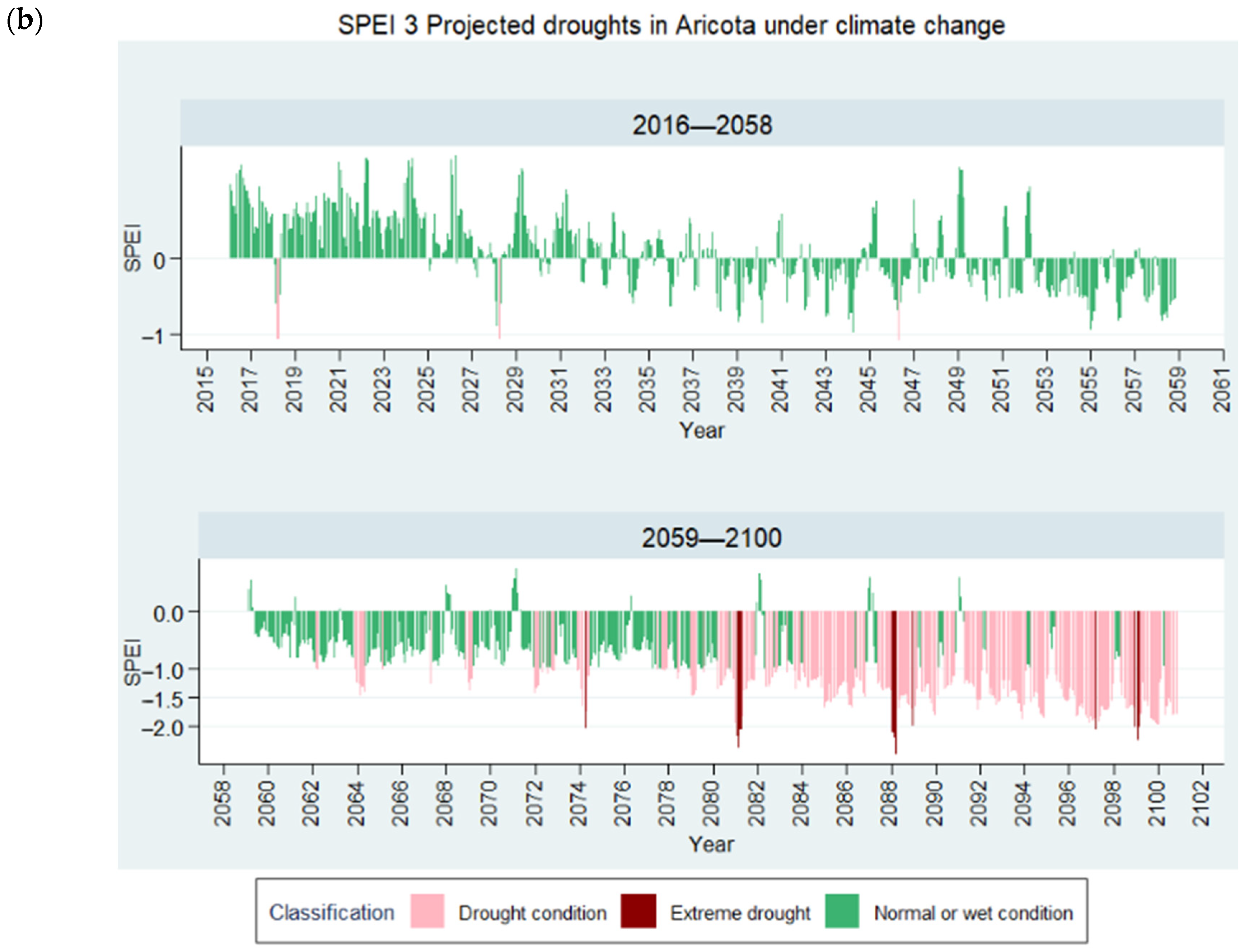
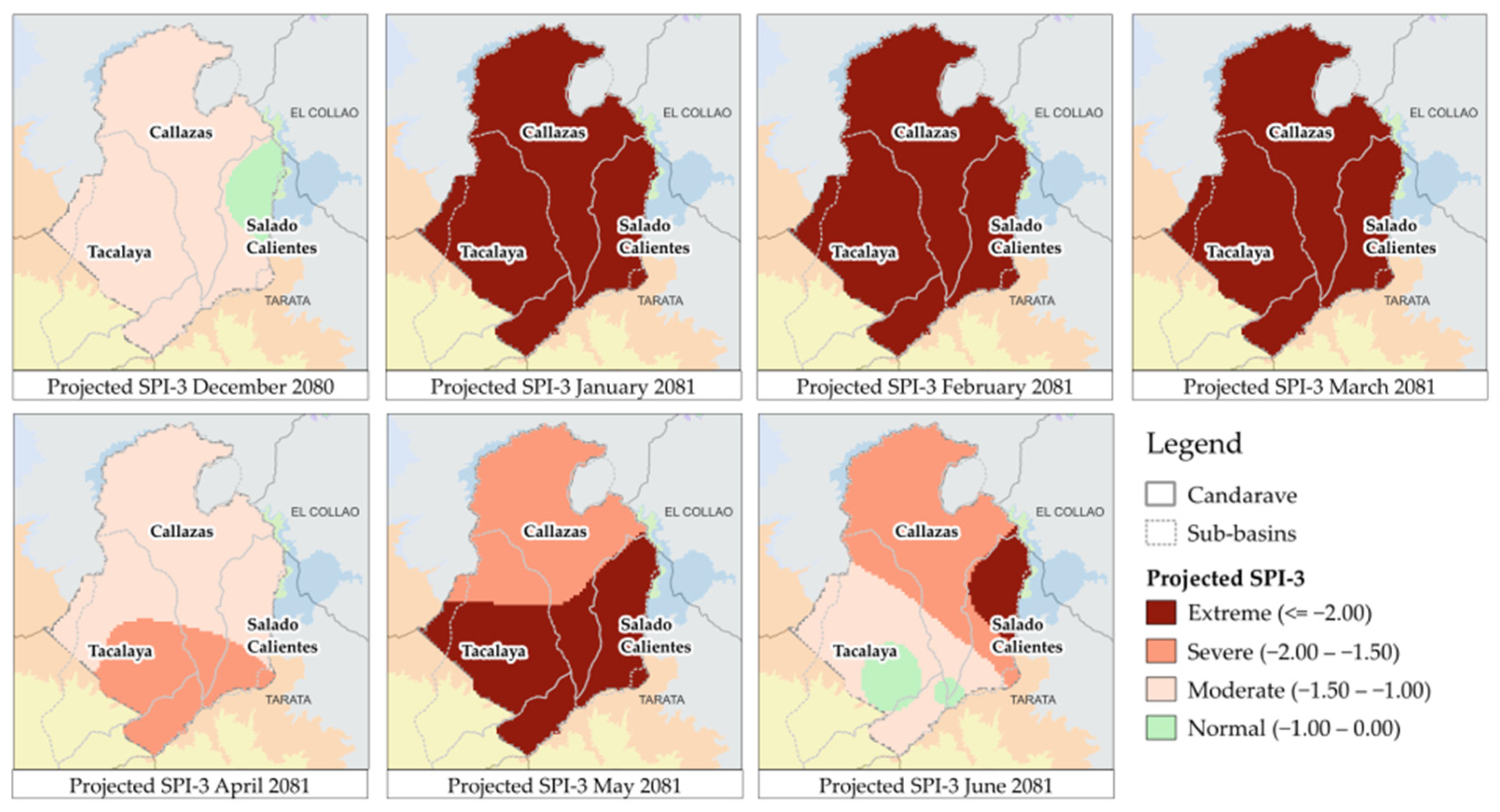
3.2.2. Projected Drought

Figure 18 shows the temporal variability of projected meteorological drought in Aricota Weather Station. Both indexes and all virtual weather stations highlight an increase in drought frequency and intensity in the last 30 years of the century; however, SPEI presents a concerning long-lasting drought scenario from 2087.

SPI-3 projected extreme drought events in 2074, 2081, 2088, 2089, and 2099. According to SPI-3, the more intense and severe droughts are those in 2081 and 2088 (

Table 12. Projected drought features at a 3-month time scale according to SPI and SPEI results.

Index	Weather Station	Start Date	End Date	Duration (Months)	Maximum Intensity	Severity
SPI-3	Aricota	May 2074	June 2074	2	−2.56	−3.68
		January 2081	June 2081	6	−3.55	−14.41
		February 2088	June 2088	5	−3.79	−10.5
		January 2089	March 2089	3	−2.68	−5.73
		January 2099	April 2099	4	−2.69	−8.21
	Cairani	May 2074	June 2074	2	−2.57	−4.38
		January 2081	June 2081	6	−3.68	−14.27
		February 2088	June 2088	5	−3.75	−10.37
		January 2089	April 2089	4	−2.68	−5.84
		January 2099	April 2099	4	−2.63	−7.9
SPEI-3	Aricota	December 2073	April 2076	29	−2.03	−25.10
		April 2080	December 2081	21	−2.38	−29.17
		June 2087	December 2090	43	−2.49	−60.70
		June 2095	December 2100	67	−2.25	−107.87
	Cairani	February 2074	February 2076	25	−2.23	−19.94
		March 2080	December 2081	21	−2.53	−32.33
		June 2087	March 2090	34	−2.63	−52.84
		June 2098	December 2100	31	−2.32	−47.76

). SPEI-3 also reported extreme droughts in those years; however, those events are longer, grouping two SPI events in one. Since SSP3-7.0 projected a steady rise in temperature toward the end of the century, it is possible to anticipate that the balance between precipitation and evapotranspiration will increasingly become negative.

The virtual weather stations generated in this study allowed for spatial analysis of the droughts using SPI-3 (Figure 19). The most severe drought (2081) began to extend from the southern area of the province and gradually lost intensity in the same way, showing a similar pattern to what occurred in 1992.

Figure 20 shows the temporal variability of projected droughts in the Aricota Weather Station. In the same way as the 3-month scale, both indexes show a trend of increasing frequency, severity, and intensity of agricultural droughts (

Table 13. Projected drought features at a 6-month time scale according to SPI and SPEI results.

Index	Weather Station	Start Date	End Date	Duration (Months)	Maximum Intensity	Severity
SPI-6	Aricota	October 2024	November 2024	2	−2.38	−4.07
		November 2035	June 2036	8	−2.27	−4.92
		November 2062	November 2062	1	−2.11	−2.11
		August 2067	October 2067	3	−2.12	−4.55
		August 2074	August 2074	1	−2.15	−2.15
		January 2081	August 2081	8	−3.52	−22.73
		February 2088	August 2088	7	−3.73	−17.4
		January 2089	July 2089	7	−2.71	−9.91
		September 2096	August 2097	12	−2.63	−15.83
		January 2099	July 2099	7	−2.65	−14.56
	Cairani	November 2035	June 2036	8	−2.27	−4.39
		December 2050	December 2050	1	−2.06	−2.06
		November 2051	December 2051	2	−2.12	−2.7
		August 2067	October 2067	3	−2.1	−4.32
		August 2074	August 2074	1	−2.14	−2.14
		January 2081	September 2081	9	−3.65	−23.03
		February 2088	July 2089	18	−3.77	−30.7
		September 2096	August 2097	12	−2.27	−13.84
		January 2099	July 2099	7	−2.63	−13.96
SPEI-6	Aricota	April 2080	February 2082	23	−2.19	−30.62
		August 2087	December 2100	161	−2.24	−234.84
	Cairani	February 2074	April 2076	27	−2.02	−22.74
		July 2080	December 2081	18	−2.41	−30.73
		August 2087	December 2090	41	−2.50	−62.56
		August 2098	December 2100	29	−2.12	−46.40

).

There will always be differences between SPI and SPEI due to the climate conditions of the area under analysis, especially because SPI does not consider the importance of evapotranspiration on droughts [3]. With increasing global warming, semiarid regions tend to present higher rates of evapotranspiration, which makes SPEI more suitable for drought monitoring in our study area [3]. This is corroborated in Figure 18b and Figure 20b, where the SPEI results show more concordance with the increase in temperature in the SSP3-7.0 scenario.

In semi-arid and arid regions, drought poses a constant threat to the sustainability of both local communities and ecosystems [53]. In these climatic zones, vegetation depends not only on precipitation and evapotranspiration but also on other factors, such as the use of groundwater [54], as in the case of wetland meadows. These types of climates are less resilient to the effects of droughts, likely because their water resources are already more stressed or limited; however, they do not need greater water demand for drought recovery [55]. A study conducted in the semi-arid Yellow Basin concluded that meteorological droughts will gradually intensify from 2040 to 2099 [6]. Additionally, research in Syria predicted severe and prolonged drought events under different emission scenarios from 2061 to 2100 [13]. Our findings also confirm previous research [56,57], which highlights concerns about future droughts in semi-arid regions.

On the other hand, one of the most important aquatic ecosystems and sources of moisture in the study area are the Andean wetland meadows (bofedales). These meadows serve as habitats for numerous plant and animal species. Supplied by groundwater runoff, they function as water flow regulators by retaining water during the wet season and releasing it during the dry season [58]. Bofedales are critical components of pastoral production systems because they provide forage year-round in areas with unimodal rainfall (a distinct wet and dry season) [58]. However, there is no climatic research in the area to contrast the findings of this study. Frequent drought events would lead to population migration because their only source of income is small agriculture and livestock farming dependent on the bofedales.

4. Conclusions

This research aimed to assess observed and projected extreme droughts in Candarave, the headwater of the Locumba Basin, using three drought indicators (SPI, SPEI, and VCI). It is significant to analyze the spatiotemporal variability of droughts in the study area due to their importance for the rest of the basin and people’s subsistence. In this study, observed droughts were assessed from 1981 to 2015, while projected droughts were obtained for the 2016 to 2100 period. A high-resolution climate projection dataset was used to project droughts under the SSP3-7.0 scenario.

Based on the climate data quality test, it was observed that the CanESM5, IPSL–CM6A–LR, and UKESM1–0–LL models did not perform well in the study area.

SPI and SPEI at a 3-month time scale detected seven episodes of observed extreme drought (1983, 1992, 1996, 1998, 2010, 2011, and 2012). At a 6-month time scale, both indices detected the same episodes as the 3-month time scale. Additionally, the use of VCI as an agricultural drought index needs to be evaluated in more detail, because, although it reflected SPEI-6 droughts, the low availability of suitable satellite images hindered the calculation of the indicator at different time scales.

SPI and SPEI at a 3-month and a 6-month time scale projected more than ten episodes of extreme droughts. Both indexes pointed out that extreme droughts will be more frequent, severe, and intense in the last 30 years of the century. This confirms previous research in similar climatic regions, which have projected more severe and frequent droughts by the end of the century.

One of the limitations of this study is the lack of weather stations in the area, particularly in the Andean zone, complicating the spatial analysis of droughts. The limited availability of minimum and maximum temperature data adds uncertainty to the climate models that project potential future droughts.

This research raises awareness about potential future droughts in the area and recommends the development of drought mitigation plans to protect the population from their disastrous consequences. Based on this study, future research should detect the areas that are more vulnerable to drought and develop a drought hazard map to identify the areas in Candarave that are most at risk.

References

1. Eslamian, S.; Eslamian, F. Handbook of Drought and Water Scarcity Principles of Drought and Water Scarcity; CRC Press: New York, NY, USA, 2017. [Google Scholar]
2. Liu, C.; Yang, C.; Yang, Q.; Wang, J. Spatiotemporal Drought Analysis by the Standardized Precipitation Index (SPI) and Standardized Precipitation Evapotranspiration Index (SPEI) in Sichuan Province, China. Sci. Rep. 2021, 11, 1280. [Google Scholar] [CrossRef] [PubMed]
3. Pei, Z.; Fang, S.; Wang, L.; Yang, W. Comparative Analysis of Drought Indicated by the SPI and SPEI at Various Timescales in Inner Mongolia, China. Water 2020, 12, 1925. [Google Scholar] [CrossRef]
4. Vicente-Serrano, S.M.; Quiring, S.M.; Peña-Gallardo, M.; Yuan, S.; Domínguez-Castro, F. A Review of Environmental Droughts: Increased Risk under Global Warming? Earth Sci. Rev. 2020, 201, 102953. [Google Scholar] [CrossRef]
5. Sadiqi, S.S.J.; Hong, E.-M.; Nam, W.-H.; Kim, T. Review: An Integrated Framework for Understanding Ecological Drought and Drought Resistance. Sci. Total Environ. 2022, 846, 157477. [Google Scholar] [CrossRef]
6. Wang, L.; Shu, Z.; Wang, G.; Sun, Z.; Yan, H.; Bao, Z. Analysis of Future Meteorological Drought Changes in the Yellow River Basin under Climate Change. Water 2022, 14, 1896. [Google Scholar] [CrossRef]
7. Fiorella, V.J. Análisis Del Riesgo de Sequías En El Sur Del Perú; Senamhi: Lima, Perú, 2016. [Google Scholar]
8. Zubieta, R.; Molina-Carpio, J.; Laqui, W.; Sulca, J.; Ilbay, M. Comparative Analysis of Climate Change Impacts on Meteorological, Hydrological, and Agricultural Droughts in the Lake Titicaca Basin. Water 2021, 13, 175. [Google Scholar] [CrossRef]
9. Shen, M.; Chen, J.; Zhuan, M.; Chen, H.; Xu, C.-Y.; Xiong, L. Estimating Uncertainty and Its Temporal Variation Related to Global Climate Models in Quantifying Climate Change Impacts on Hydrology. J. Hydrol. 2018, 556, 10–24. [Google Scholar] [CrossRef]
10. Viloria, J.A.; Olivares, B.O.; García, P.; Paredes-Trejo, F.; Rosales, A. Mapping Projected Variations of Temperature and Precipitation Due to Climate Change in Venezuela. Hydrology 2023, 10, 96. [Google Scholar] [CrossRef]
11. Zhang, Y.; Fu, B.; Feng, X.; Pan, N. Response of Ecohydrological Variables to Meteorological Drought under Climate Change. Remote Sens. 2022, 14, 1920. [Google Scholar] [CrossRef]
12. Xu, F.; Bento, V.A.; Qu, Y.; Wang, Q. Projections of Global Drought and Their Climate Drivers Using CMIP6 Global Climate Models. Water 2023, 15, 2272. [Google Scholar] [CrossRef]
13. Mathbout, S.; Martin-Vide, J.; Bustins, J.A.L. Drought Characteristics Projections Based on CMIP6 Climate Change Scenarios in Syria. J. Hydrol. Reg. Stud. 2023, 50, 101581. [Google Scholar] [CrossRef]
14. Abara, M.; Komariah; Budiastuti, S. Drought Frequency, Severity, and Duration Monitoring Based on Climate Change in Southern and Southeastern Ethiopia. In IOP Conference Series: Earth and Environmental Science; IOP Publishing: Bristol, UK, 2020; Volume 477, p. 012011. [Google Scholar] [CrossRef]
15. Liu, X.; Zhu, X.; Pan, Y.; Bai, J.; Li, S. Performance of Different Drought Indices for Agriculture Drought in the North China Plain. J. Arid Land 2018, 10, 507–516. [Google Scholar] [CrossRef]
16. Montes-Vega, M.J.; Guardiola-Albert, C.; Rodríguez-Rodríguez, M. Calculation of the SPI, SPEI, and GRDI Indices for Historical Climatic Data from Doñana National Park: Forecasting Climatic Series (2030–2059) Using Two Climatic Scenarios RCP 4.5 and RCP 8.5 by IPCC. Water 2023, 15, 2369. [Google Scholar] [CrossRef]
17. Senhorelo, A.P.; Sousa, E.F.; Santos, A.R.D.; Ferrari, J.L.; Peluzio, J.B.E.; Zanetti, S.S.; Carvalho, R.d.C.F.; Camargo Filho, C.B.; Barbosa de Souza, K.; Moreira, T.R.; et al. Application of the Vegetation Condition Index in the Diagnosis of Spatiotemporal Distribution of Agricultural Droughts: A Case Study Concerning the State of Espírito Santo, Southeastern Brazil. Diversity 2023, 15, 460. [Google Scholar] [CrossRef]
18. Sh, S. Comparison of the Vegetation Condition Index with Meteorological Drought Indices:A Case Study in Henan Province. J. Glaciol. Geocryol. 2013, 35, 990–998. [Google Scholar]
19. Fiorella, V.J. Regionalización y Caracterización de Sequías En El Perú; Senamshi: Lima, Perú, 2015. [Google Scholar]
20. Chucuya, S.; Vera, A.; Pino-Vargas, E.; Steenken, A.; Mahlknecht, J.; Montalván, I. Hydrogeochemical Characterization and Identification of Factors Influencing Groundwater Quality in Coastal Aquifers, Case: La Yarada, Tacna, Peru. Int. J. Environ. Res. Public Health 2022, 19, 2815. [Google Scholar] [CrossRef]
21. Pocco, V.; Chucuya, S.; Huayna, G.; Ingol-Blanco, E.; Pino-Vargas, E. A Multi-Criteria Decision-Making Technique Using Remote Sensors to Evaluate the Potential of Groundwater in the Arid Zone Basin of the Atacama Desert. Water 2023, 15, 1344. [Google Scholar] [CrossRef]
22. Consorcio, R.L. Estudio de Los Recursos Hídricos Superficiales y Subterráneos e Infraestructura Hidráulica Para El Plan de Aprovechamiento En La Cuenca Del Río Locumba, En La Región de Tacna; Autoridad Nacional del Agua: Lima, Perú, 2016. [Google Scholar]
23. Pino-Vargas, E.; Chávarri-Velarde, E.; Ingol-Blanco, E.; Mejía, F.; Cruz, A.; Vera, A. Impacts of Climate Change and Variability on Precipitation and Maximum Flows in Devil’s Creek, Tacna, Peru. Hydrology 2022, 9, 10. [Google Scholar] [CrossRef]
24. Fernandez-Palomino, C.A.; Hattermann, F.F.; Krysanova, A.L.; Vega-Jácome, F.; Lavado, W.; Santini, W.; Aybar, C.; Bronstert, A. A Novel High-Resolution Gridded Precipitation Dataset for Peruvian and Ecuadorian Watersheds–Development and Hydrological Evaluation. J. Hydrometeorol. 2021, 23, 309–336. [Google Scholar] [CrossRef]
25. Llauca, H.; Lavado-Casimiro, W.; Montesinos, C.; Santini, W.; Rau, P. PISCO_HyM_GR2M: A Model of Monthly Water Balance in Peru (1981–2020). Water 2021, 13, 1048. [Google Scholar] [CrossRef]
26. Fernandez-Palomino, C.A.; Hattermann, F.F.; Krysanova, V.; Vega-Jácome, F.; Menz, C.; Gleixner, S.; Bronstert, A. High-Resolution Climate Projection Dataset Based on CMIP6 for Peru and Ecuador: BASD-CMIP6-PE. Sci. Data 2024, 11, 34. [Google Scholar] [CrossRef] [PubMed]
27. Escoto Castillo, A.; Sánchez Peña, L.; Gachuz Delgado, S. Shared Socioeconomic Pathways (SSP): New Ways to Assess Climate and Social Change. Estud. Demogr. Urbanos Col. Mex. 2017, 32, 669–693. [Google Scholar] [CrossRef]
28. Quille-Mamani, J.A.; Huayna, G.; Pino-Vargas, E.; Chucuya-Mamani, S.; Vera-Barrios, B.; Ramos-Fernandez, L.; Espinoza-Molina, J.; Cabrera-Olivera, F. Spatio-Temporal Evolution of Olive Tree Water Status Using Land Surface Temperature and Vegetation Indices Derived from Landsat 5 and 8 Satellite Imagery in Southern Peru. Agriculture 2024, 14, 662. [Google Scholar] [CrossRef]
29. Searcy, J.K.; Hardison, C.H. Double-Mass Curves; United States Department of the Interior: Washington, DC, USA, 1960. [Google Scholar]
30. Urrutia-Mosquera, J. Metodología Para La Imputación de Datos Faltantes En Metereología. Lex Sci. 2010, 3, 44–49. [Google Scholar]
31. Kocsis, T.; Kovács-Székely, I.; Anda, A. Homogeneity Tests and Non-Parametric Analyses of Tendencies in Precipitation Time Series in Keszthely, Western Hungary. Theor. Appl. Climatol. 2020, 139, 849–859. [Google Scholar] [CrossRef]
32. Wang, X.; Yang, J.; Xiong, J.; Shen, G.; Yong, Z.; Sun, H.; He, W.; Luo, S.; Cui, X. Investigating the Impact of the Spatiotemporal Bias Correction of Precipitation in CMIP6 Climate Models on Drought Assessments. Remote Sens. 2022, 14, 6172. [Google Scholar] [CrossRef]
33. Taylor, K.E. Summarizing Multiple Aspects of Model Performance in a Single Diagram. J. Geophys. Res. Atmos. 2001, 106, 7183–7192. [Google Scholar] [CrossRef]
34. Lei, X.; Xu, C.; Liu, F.; Song, L.; Cao, L.; Suo, N. Evaluation of CMIP6 Models and Multi-Model Ensemble for Extreme Precipitation over Arid Central Asia. Remote Sens. 2023, 15, 2376. [Google Scholar] [CrossRef]
35. Pramudya, Y.; Onishi, T. Assessment of the Standardized Precipitation Index (SPI) in Tegal City, Central Java, Indonesia. In IOP Conference Series: Earth and Environmental Science; IOP Publishing: Bristol, UK, 2018; Volume 129, p. 012019. [Google Scholar] [CrossRef]
36. Tsesmelis, D.E.; Vasilakou, C.G.; Kalogeropoulos, K.; Stathopoulos, N.; Alexandris, S.G.; Zervas, E.; Oikonomou, P.D.; Karavitis, C.A. Drought Assessment Using the Standardized Precipitation Index (SPI) in GIS Environment in Greece. In Computers in Earth and Environmental Sciences: Artificial Intelligence and Advanced Technologies in Hazards and Risk Management; Elsevier: Amsterdam, The Netherlands, 2021; pp. 619–633. [Google Scholar] [CrossRef]
37. Fassouli, V.P.; Karavitis, C.A.; Tsesmelis, D.E.; Alexandris, S.G. Factual Drought Index (FDI): A Composite Index Based on Precipitation and Evapotranspiration. Hydrol. Sci. J. 2021, 66, 1638–1652. [Google Scholar] [CrossRef]
38. Wagesho, N.; Claire, M. Analysis of Rainfall Intensity-Duration-Frequency Relationship for Rwanda. J. Water Resour. Prot. 2016, 08, 706–723. [Google Scholar] [CrossRef]
39. Karavitis, C.A.; Alexandris, S.; Tsesmelis, D.E.; Athanasopoulos, G. Application of the Standardized Precipitation Index (SPI) in Greece. Water 2011, 3, 787–805. [Google Scholar] [CrossRef]
40. Endara, S.; Acuña, J.; Vega, F.; Febre, C.; Correa, K.; Ávalos, G. Caracterización Espacio Temporal de La Sequía En Los Departamentos Altoandinos Del Perú (1981–2018); Senamhi: Lima, Perú, 2019. [Google Scholar]
41. Thom, H.C. A Note on the Gamma Distribution. Mon. Weather Rev. 1958, 86, 117–122. [Google Scholar] [CrossRef]
42. Şenaut, Z. Applied Drought Modeling, Prediction, and Mitigation; Elsevier: Amsterdam, The Netherlands, 2015; ISBN 9780128021767. [Google Scholar]
43. National Drought Mitigation Center. SPI Generator [Software]; University of Nebraska–Lincoln: Lincoln, NE, USA, 2018. [Google Scholar]
44. Vicente-Serrano, S.M.; Beguería, S.; López-Moreno, J.I. A Multiscalar Drought Index Sensitive to Global Warming: The Standardized Precipitation Evapotranspiration Index. J. Clim. 2010, 23, 1696–1718. [Google Scholar] [CrossRef]
45. Orimoloye, I.R.; Belle, J.A.; Orimoloye, Y.M.; Olusola, A.O.; Ololade, O.O. Drought: A Common Environmental Disaster. Atmosphere 2022, 13, 111. [Google Scholar] [CrossRef]
46. Mupepi, O.; Matsa, M.M. A Combination of Vegetation Condition Index, Standardized Precipitation Index and Human Observation in Monitoring Spatio-Temporal Dynamics of Drought. A Case of Zvishavane District in Zimbabwe. Environ. Dev. 2023, 45, 100802. [Google Scholar] [CrossRef]
47. Liang, L.; Qiu, S.; Yan, J.; Shi, Y.; Geng, D. VCI-Based Analysis on Spatiotemporal Variations of Spring Drought in China. Int. J. Environ. Res. Public Health 2021, 18, 7967. [Google Scholar] [CrossRef]
48. Vincent, L.A.; Mekis, E. Discontinuities Due to Joining Precipitation Station Observations in Canada. J. Appl. Meteorol. Clim. 2009, 48, 156–166. [Google Scholar] [CrossRef]
49. Rascón, J.; Gosgot Angeles, W.; Quiñones Huatangari, L.; Oliva, M.; Barrena Gurbillón, M.Á. Dry and Wet Events in Andean Populations of Northern Peru: A Case Study of Chachapoyas, Peru. Front Environ. Sci. 2021, 9, 614438. [Google Scholar] [CrossRef]
50. Akter, M.L.; Rahman, M.N.; Azim, S.A.; Rony, M.R.H.; Sohel, M.D.S.; Abdo, H.G. Estimation of Drought Trends and Comparison between SPI and SPEI with Prediction Using Machine Learning Models in Rangpur, Bangladesh. Geol. Ecol. Landsc. 2023, 1–15. [Google Scholar] [CrossRef]
51. Meseguer-Ruiz, O.; Serrano-Notivoli, R.; Aránguiz-Acuña, A.; Fuentealba, M.; Nuñez-Hidalgo, I.; Sarricolea, P.; Garreaud, R. Comparing SPI and SPEI to Detect Different Precipitation and Temperature Regimes in Chile throughout the Last Four Decades. Atmos. Res. 2024, 297, 107085. [Google Scholar] [CrossRef]
52. Andujar, E.; Krakauer, N.Y.; Yi, C.; Kogan, F. Ecosystem Drought Response Timescales from Thermal Emission versus Shortwave Remote Sensing. Adv. Meteorol. 2017, 2017, 8434020. [Google Scholar] [CrossRef]
53. Patel, R.; Patel, A. Evaluating the Impact of Climate Change on Drought Risk in Semi-Arid Region Using GIS Technique. Results Eng. 2024, 21, 101957. [Google Scholar] [CrossRef]
54. Hamarash, H.; Hamad, R.; Rasul, A. Meteorological Drought in Semi-Arid Regions: A Case Study of Iran. J. Arid Land 2022, 14, 1212–1233. [Google Scholar] [CrossRef]
55. Lan, X.; Liu, Z.; Ge, Y.; Yan, Y.; She, Z.; Cheng, L.; Chen, X. Semi-Arid Rather than Arid Regions of China Deserve the Priority in Drought Mitigation Efforts. J. Hydrol. 2024, 641, 131791. [Google Scholar] [CrossRef]
56. Li, J.; Miao, C.; Wei, W.; Zhang, G.; Hua, L.; Chen, Y.; Wang, X. Evaluation of CMIP6 Global Climate Models for Simulating Land Surface Energy and Water Fluxes During 1979–2014. J. Adv. Model. Earth Syst. 2021, 13, e2021MS002515. [Google Scholar] [CrossRef]
57. Zhai, J.; Mondal, S.K.; Fischer, T.; Wang, Y.; Su, B.; Huang, J.; Tao, H.; Wang, G.; Ullah, W.; Uddin, M.J. Future Drought Characteristics through a Multi-Model Ensemble from CMIP6 over South Asia. Atmos. Res. 2020, 246, 105111. [Google Scholar] [CrossRef]
58. Franco León, P.; Sulca Quispe, L. Evaluación Socio-Ambiental Del Bofedal Huaytire de La Provincia de Candarave-Tacna. Cienc. Desarro. 2019, 12, 93–98. [Google Scholar] [CrossRef]
Figure 1. Location and climate classification of Candarave.
Atmosphere 16 00018 g001
Figure 2. Average maximum temperature, minimum temperature, and rainfall in Aricota.
Atmosphere 16 00018 g002
Figure 3. Homogeneous drought regions in Peru based on the SPI. Source: [19].
Atmosphere 16 00018 g003
Figure 4. Flowchart of the methodology followed in this study.
Atmosphere 16 00018 g004
Figure 5. Grouping of virtual weather stations according to climatic zone and altitude.
Atmosphere 16 00018 g005
Figure 6. Results roadmap.
Atmosphere 16 00018 g006
Figure 7. Correlation between gridded datasets and observed precipitation data.
Atmosphere 16 00018 g007
Figure 8. Double mass curves: (a) Aricota and Cairani Weather Stations; (b) Vilacota and Titijones Weather Stations.
Atmosphere 16 00018 g008
Figure 9. Total annual rainfall series at Titijones Weather Station showing a changing point (step) in 1996.
Atmosphere 16 00018 g009
Figure 10. Rainfall series at Titijones Weather Station showing homogeneity of the data.
Atmosphere 16 00018 g010
Figure 11. Taylor diagram for precipitation variable: (a) Aricota Weather Station; (b) Cairani Weather Station.
Atmosphere 16 00018 g011
Figure 12. Taylor diagram for maximum temperature variable: (a) Aricota Weather Station; (b) Cairani Weather Station.
Atmosphere 16 00018 g012
Figure 13. Taylor diagram for minimum temperature variable: (a) Aricota Weather Station; (b) Cairani Weather Station.
Atmosphere 16 00018 g013
Figure 14. Observed droughts in Aricota. (a) SPI-3; (b) SPEI-3.
Atmosphere 16 00018 g014
Figure 15. Spatial variability of the extreme drought that occurred in 1992.
Atmosphere 16 00018 g015
Figure 16. Observed droughts in Aricota. (a) SPI-6; (b) SPEI-6.
Atmosphere 16 00018 g016
Figure 17. VCI-1 for 1996.
Atmosphere 16 00018 g017
Figure 18. Projected droughts in Aricota. (a) SPI-3; (b) SPEI-3.
Atmosphere 16 00018 g018aAtmosphere 16 00018 g018b
Figure 19. Spatial variability of the most extreme projected drought in 2081.
Atmosphere 16 00018 g019
Figure 20. Projected droughts in Aricota. (a) SPI-6; (b) SPEI-6.
Atmosphere 16 00018 g020