Abstract
A machine learning algorithm combined with measurements obtained by a NILU-UV irradiance meter enables the determination of total ozone column (TOC) amount and cloud optical depth (COD). In the New York City area, a NILU-UV instrument on the rooftop of a Stevens Institute of Technology building (40.74° N, −74.03° E) has been used to collect data for several years. Inspired by a previous study [Opt. Express 22, 19595 (2014)], this research presents an updated neural-network-based method for TOC and COD retrievals. This method provides reliable results under heavy cloud conditions, and a convenient algorithm for the simultaneous retrieval of TOC and COD values. The TOC values are presented for 2014–2023, and both were compared with results obtained using the look-up table (LUT) method and measurements by the Ozone Monitoring Instrument (OMI), deployed on NASA’s AURA satellite. COD results are also provided.
1. Introduction
Atmospheric ozone plays a crucial role in absorbing ultraviolet (UV) radiation, thus providing protection of the biosphere, which encompasses all living organisms and ecosystems. While a moderate amount of UV radiation can stimulate vitamin D production in the skin, excessive exposure to UV radiation poses risks to both humans and most organisms [1]. Thus, monitoring the total ozone column (TOC) amount is important, providing a strong motivation and incentive to develop improved satellite and ground-based TOC retrieval techniques. Recently, machine learning techniques and neural networks [2] have been successfully applied in many fields of the natural sciences. Neural networks have great flexibility and potential to address a variety of problems in cognitive science, information science, computer science, marketing, artificial intelligence, biology, and chemistry.
In 2013, the latest TOC and COD results for the New York City area were reported, derived using a radial basis function neural network [3]. Since then, new developments have been made in radiative transfer simulations, machine learning, and computer hardware. The two main motivators of this study are (i) to follow up on the state and trends of the ozone layer in this area for the time period 2014–2024, and (ii) to create an updated machine learning-based retrieval technique that is accurate and easy to use.
The main instruments used in this research are the NILU-UV (No. 115), which has been deployed and operated in the New York City area (40.74° N, −74.03° E) for eleven years (2014–2024), and the Ozone Monitoring Instrument (OMI).
A detailed description of the radiative transfer simulations, retrieval methodology, machine learning and training methods used in this research is provided in the following sections. Furthermore, comparisons of results obtained by the neural network and LUT methods applied to the NILU-UV data and the OMI results as well as the relationship between the radiation modification factor (RMF) and COD are presented and discussed.
2. Methodology
A combination of radiative transfer simulations based on AccuRT [4], machine learning methods and irradiance measurements has been used to infer TOC and COD values. First, radiative transfer simulations were used to create synthetic training data for a neural network. After establishing the neural network, we used the synthetic dataset, with the absolute response functions of the NILU-UV applied to it, for training. Once the training was completed, we undertook the validation of the results. This step was followed by the preparation of the collected NILU-UV raw data to be used as input to the neural network for obtaining the TOC and COD values. Once the TOC results had been obtained, they were compared to the OMI values, and statistics were calculated to quantify their similarities/discrepancies. In the following sections, we describe (i) the instrumentation, (ii) the radiative transfer simulations, (iii) the neural network approach, (iv) the NILU-UV and OMI data preparation, (v) the results of our research, and finally, (vi) our conclusions.
3. Instrumentation
3.1. NILU-UV
The NILU-UV No. 115 irradiance radiometer was used to collect the data employed in this research. The NILU-UV radiometer measures voltages in six channels, each depending on the magnitude of the downward irradiance of that channel, its bandwidth, and its spectral response function. Five channels of the NILU-UV instrument are centered at, respectively, 302 nm, 312 nm, 320 nm, 340 nm and 380 nm, each having a full width at half maximum (FWHM) of approximately 10 nm. A sixth channel takes measurements in the visible (or so-called photosynthetically active) spectral range, 400–700 nm, with a bandwidth of 300 nm at FWHM. For the five UV channels, the range of the absolute response function of the NILU-UV spans wavelengths from 290 nm to 387 nm. The NILU-UV instrument No. 115 was optically characterized (spectral and cosine responses) at the optical laboratory of the Norwegian Radiation and Nuclear Safety Authority (DSA) [5]. Figure 1 shows the absolute response functions for each channel.
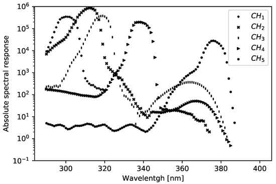
Figure 1.
The absolute spectral response of No. 115 NILU-UV instrument.
The response functions were characterized with a 1 nm resolution. Throughout this study, channels 1, 3 and 5 were used. Channel 3 is significantly less sensitive to ozone abundance than channel 1, so the ratio of the two is a good choice for TOC amount retrieval. At (channel 5), the ozone cross-section is near minimal. Therefore, channel 5 is relatively insensitive to ozone but is responsive to clouds, aerosol particles, and surface albedo. Hence, channel 5 is optimal for quantifying the impact of clouds, aerosols and surface reflection on the measured radiation field through the radiation modification factor (RMF) defined in Equation (1) below. The absolute response of these channels span over the whole range mentioned above, i.e., 290 nm nm with a 1 nm resolution.
The radiometer has built-in memory to store data and a temperature controller. It records data at a 1-min time resolution. The built-in memory has a limited capacity of about 24 days, but data can be recorded and stored by connecting the device to a computer with a RS-232 port. The instrument is equipped with moderate bandwidth filters that tend to drift with time; hence, the instrument requires a relative calibration (typically once or twice a month). The total weight of the instrument is 3.3 kg; it is waterproof and designed to operate in harsh environments.
3.2. OMI
The Ozone Monitoring Instrument (OMI) is deployed on NASA’s AURA satellite, which is in a sun-synchronous orbit. This satellite was launched on 15 July 2004. The OMI measures UV radiation in several wavelength bands that is used to infer TOC amounts and aerosol abundance. OMI data are gridded at 0.25 degrees, it has a 780 × 576 (spectral × spatial) pixel CCD detector. AURA’s swath is 2600 km and the nadir viewing footprint is 13 km × 24 km [6].
4. Radiative Transfer Simulations
In order to train the neural network, one needs to provide training data to the algorithm. To create a suitable training (or synthetic) dataset, we used AccuRT [4], which is a unique, state of the art radiative transfer simulation package that was designed to provide a reliable, well-tested, robust, versatile, and easy-to-use radiation transfer tool for coupled (atmosphere and underlying surface) systems. AccuRT uses the discrete ordinate method for the radiative transfer modeling.
The desired outputs from the neural network are the TOC amount and the COD at 380 nm (). The available possible inputs from the NILU-UV are the raw measurements from its six channels, and the so-called radiation modification factor (RMF) inferred from the measurements, as follows.
From [7]: “When solar radiation passes through the ozone layer of the atmosphere, a portion of the UV radiation will be absorbed by ozone, while the portion that penetrates the ozone layer will be multiply scattered or absorbed by air molecules, aerosols, and cloud particles. To take into account the effects of clouds, aerosol particles, and surface albedo on the UV radiation a radiation modification factor (RMF) is introduced. The RMF is the measured irradiance at wavelength and solar zenith angle , , divided by the calculated irradiance, , at the same , , and TOC at the instrument location for a cloud- and aerosol-free sky and for zero surface albedo”:
In this study, the 380 nm channel was used to determine the RMF. As already mentioned, the RMF is relatively insensitive to the ozone abundance because the ozone absorption cross-section is very small at 380 nm, but sensitive to clouds, aerosol particles, and the surface albedo. “The RMF may be larger than 100 when broken clouds are present and the direct beam from the unobscured Sun is measured by the instrument as well as diffuse sky radiation scattered by broken clouds” [8].
The goal was to train the neural network in terms of the measured voltages in each channel at different atmospheric conditions for varying COD () values, TOC amounts, and solar zenith angles . Hence, the solar spectrum (290 nm–387 nm) and the resolution of the absolute response functions (1 nm) were used in the AccuRT computations to obtain the irradiances at these wavelengths.
The cloud optical depth (COD) is not used as a direct input to AccuRT. Instead, the cloud volume fraction () is used in conjunction with the cloud extinction coefficient to generate the cloud optical depth at 380 nm, . The relationship between the cloud volume fraction () and the cloud optical depth is shown in Figure 2 below.
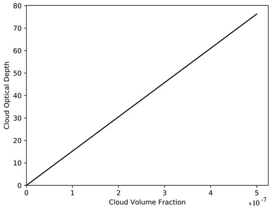
Figure 2.
Cloud optical depth versus cloud volume fraction .
The input parameters and their ranges are shown in Table 1. A total of 20,000 simulations were prepared to be computed. For each simulation, a value was randomly selected for , O3, and within the ranges presented in Table 1. A MATLAB [9] script was used to cycle through the 20,000 prearranged cases and run the individual AccuRT simulations.

Table 1.
Input parameters and their ranges for the AccuRT simulations.
For the simulations, the US Standard Atmosphere [10] model was used and the surface albedo was chosen to be 0.14, which is typical for cities [11]. The location-specific aerosol size distribution and fine and coarse mode values were adopted from our previous research [12]. The aerosol particles were placed between 0 and 2000 m with the volume fraction set to . The COD retrieval sensitivity assessment is given in Section 7.2. With the cloud model used (see Section 4), the limits of are equivalent to min and max in terms of COD. In Table 1, min reflects the lowest possible solar zenith angle at the measurement site, and max the upper limit to minimize measurement error. The minimum of was chosen to be the lowest solar zenith angle throughout the year and the maximum limit was selected to be to accommodate the slab geometry used in the calculations, in which the curvature of the atmosphere is not accounted for, and to keep measurement errors low. For , the impact of cloudiness, the vertical profile of ozone and temperature, the imperfect cosine response of the instrument, and the absolute calibration error reduce the accuracy of the results [13].
Cloud Model
Clouds were assumed to consist of a collection of homogeneous water spheres having a single-mode log-normal volume size distribution with a specified volume mode radius μm and width . Clouds were placed between 2000 m and 4000 m altitude, and a Mie code was used to compute the inherent optical properties of cloud particles. To convert the cloud volume fraction to cloud optical depth, repeated AccuRT simulations were conducted to obtain at different cloud volume fractions. The results are shown in Figure 2. The exact formulation of the relationship between versus is presented in Appendix A.
The relationship between the RMF and was investigated. Using AccuRT to calculate irradiance at 380 nm for different values yielded the theoretical relationship between RMF and as shown in Figure 3.
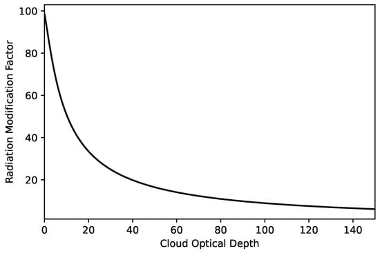
Figure 3.
Modeled relation between RMF and .
5. Neural Network
A machine learning algorithm based on a multi-layer neural network (MLNN) [14] was built with three hidden layers consisting of 100, 90 and 75 neurons using the scikit-learn Python 3 library [15]. To deal with the large data range and to improve the training performance, logarithmic scaling was performed, except for the solar zenith angle, where the cosine of the angle was used. An adaptive learning rate was applied to the training with hyperbolic tangent activation functions. The Adam optimizer [16] was applied with a validation tolerance limit of and a 0.1 validation fraction. To prevent overfitting, early stopping was applied. It took about 90 iterations to train the network.
The predecessor of our present method was based on a radial basis function neural network (RBFNN) [17] that needed experimentation for optimization as described by Fan et al. (2014) [3]. This “manual” interaction to tune the RBFNN is not needed in our MLNN approach, providing increased practicality and ease of use. In terms of training and retrieval, Fan et al. (2014) [3] used irradiances, while our MLNN was trained on simulated measured voltages, as described in Section 5.1. The TOC and COD retrievals are also based on the voltages measured by the NILU-UV instrument. The training data preparation and the two types of validation are described below.
5.1. Training Data
Besides taking the cosine of the solar zenith angle , to prepare the inputs () for the neural network training, the simulated irradiances were convolved with the absolute response functions of the corresponding NILU-UV channels. Here, i denotes the channel number. This transformation yields the corresponding voltages that would be measured in the NILU-UV channels. For channels 1, 3 and 5, the convolutions were as follows:
where the summation is carried out using a wavelength step of 1 nm.
The ratio of voltages in two channels was used for the TOC retrieval. As a reminder, our goal is to retrieve TOC and (COD at 380 nm). The inputs and outputs of the neural network are shown in Table 2.

Table 2.
Input and output parameters of the neural network.
5.2. Holdout Validation
Holdout validation involves splitting the dataset into two separate sets: one for training the model and one for testing it. The K-fold validation divides the dataset into K equal parts, or “folds”. The model is trained and tested K times, each time using a different fold as the test set and the remaining folds as the training set. This approach ensures that every data point is used for both training and validation. After data processing, and setting up the training (defining loss function, selecting an optimizer, determining the learning rate and number of neurons), the neural network was ready for the supervised learning and the synthetic data were applied for the training. To validate the results, two procedures were used. First, a 75:25 holdout, and then, a K-fold validation for (see Section 5.3) was applied. For the holdout method [18] (Section 8.2.2), the mean percent error (PE), the mean absolute percent error (APE) and the squared correlation coefficient ( were calculated using 5000 data points of the neural network (MLNN) predictions versus the modeled results described in Section 4. The APE and PE are defined as follows:
and
where and are the results from the neural network and radiative transfer simulations (Section 4 model), respectively, for the i-th set of parameters, or i-th case, represented by the input array . The results predicted by the trained neural network vs. the simulated values are plotted in Figure 4 and Figure 5.
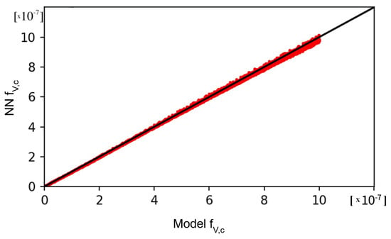
Figure 4.
Cloud volume fraction results by the MLNN vs. modeled values.
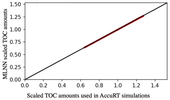
Figure 5.
Scaled TOC by the MLNN vs. the modeled values.
In Figure 5, the red color indicates the values from the trained MLNN and the model data. The x-axis represents the scaled TOC amounts used in AccuRT for the simulations. The TOC amount is scaled to the standard US atmosphere [10], where the equivalent TOC depth is m, which in Dobson units corresponds to 345 DU. The lower and upper limits of the modeled TOC amounts (220 DU, 440 DU) correspond to 0.6377 and 1.2754, respectively, in terms of scaled ozone amounts. The strong correlation between the data points is evident from Figure 4, Figure 5, the high value, and the low error rates. The calculated statistical parameters are provided in Table 3.

Table 3.
Statistical results of the neural network validation, calculated using 5000 data points from the modeled and MLNN-predicted values.
5.3. K-Fold Validation
A K-fold cross-validation [19] was also performed on the training data to see how they perform on “unseen” data. A standard cross-validation technique is based on partitioning a portion of the training data and utilizing it to generate predictions from the neural network. The resulting error estimation provides insight into how the model performs on unseen data (or validation set). This technique is commonly referred to as the holdout method, a simple form of cross-validation. In this case, was adopted, which is a common choice for this kind of validation method. K-fold cross-validation is a technique where the dataset is divided into K subsets. The holdout method is repeated K times, in which each subset is used once as the validation set and the remaining subsets are combined to form the training set. The error estimation is averaged over all K trials to determine the overall effectiveness of our model. This approach ensures that each data point is included only once in the validation set and in the training set times. Swapping the training and test sets further enhances the efficacy of this method. In this case, each time ( times), 16,000 data points were used for training and 4000 for validation. The statistical results for the K-fold cross-validation are provided in Table 4.

Table 4.
Statistical results of the neural network K-fold cross-validation using .
The values for both O3 and at 380 nm are 0.999, demonstrating high correlation between the predicted and simulated values. This high correlation indicates that the model explains almost all of the variability in the data. The percentage errors for O3 and are low, reflecting the model’s high accuracy. The negative PE value reveals a slight underestimation of COD by the MLNN in both Table 3 and Table 4. The low APE-s for O3 and suggests that the model performs accurately. Overall, the neural network model exhibits good performance for both variables, with high values and low errors.
6. NILU-UV and OMI Data Preparation
Once the MLNN had been trained and validated, the preparation of the NILU-UV raw data was performed. Unfortunately, some of the measurements were erroneous as the instrument occasionally logged faulty data. Missing data points, unfinished readings and the appearance of random characters were the most common occurrences of faulty data. These NILU-UV data were removed from the dataset before the following steps were taken.
The NILU-UV instrument registers the timestamps in UTC time. First, the solar zenith angle is calculated based on the location and time. The other two pieces of information needed are the ratio and , where stands for channel reading. As mentioned in Section 3b in [7], the drift factor for each channel needs to be used to compensate for the degradation of the Teflon diffuser of the instrument. The drift data nearest to the measurement time were always used to take instrument drift into account. The imperfect cosine response of the instrument was also accounted for by dividing the measured signal in each channel with the corresponding cosine correction value, as described in Section 3 in [8]. The cosine response functions are provided in Figure A5 in the Appendix A. A schematic illustration of the full retrieval methodology is provided in Figure 6.

Figure 6.
Schematic illustration of the retrieval methodology.
There were some missing data in the available dataset for the years 2014–2019, mainly for the year 2016. Approximately the first third and last third portions of the data were lacking from 2017 and 2019, respectively. Unfortunately, because of technical difficulties, NILU-UV data collected after 2019 had significant gaps of missing data.
Level 3 OMI data were acquired from NASA’s Goddard Earth Sciences Data and Information Services Center (GESDISC) in hierarchical data format (release 5) for the years of interest.
7. Results
7.1. TOC Results
The retrieved TOC amounts from the NILU-UV and OMI measurements versus day of the year are plotted for the years 2014, 2015, 2018 and 2019 in Figure 7a–d. Plots for the years 2016 and 2017 are provided in the Appendix A.
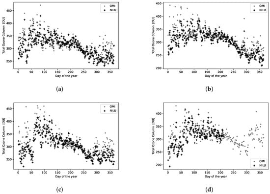
Figure 7.
TOC amounts from OMI (gray dots) and NILU-UV (black crosses) versus day of the year for (a): 2014; (b): 2015; (c): 2018; and (d): 2019.
The results in Figure 7a–d show that TOC amounts retrieved from NILU-UV measurements tend to be lower than the corresponding amounts derived from OMI measurements (see Table 5). The same tendency was observed in Section 6 in [7], and, as stated, this tendency might indicate a solar zenith angle-related error either in NILU-UV or OMI measurements.

Table 5.
Annual TOC statistical results for the years 2014–2019.
For large COD values ( > 100), the NILU-UV measurements show unrealistically low TOC values. This phenomenon has already been noticed by Dahlback [20], who showed the following observations: (i) For clouds located between 2 and 4 km with an optical depth of at zero surface albedo, the error in the calculated TOC is less than 2 DU when the LUT is computed for a cloudless sky overlying a black surface. (ii) The error will increase with increasing surface albedo. For a cloud between 2 and 4 km with an optical depth of and a surface albedo of 0.8, the error will be larger than in the case of zero surface albedo, but it will not exceed 20 DU. (iii) For a COD value of and a surface albedo of 0.8, NILU-UV measurements will give an underestimate of the TOC amount by about 6% [8]. As mentioned in Section 4, in our simulations, the surface albedo was adopted to be 0.14 and the COD value () occasionally exceeded 50.
Because the above-mentioned underestimation of TOC amounts occurred when the NILU-UV data analysis was carried out using both the look-up table method and our neural-network-based method, it may have been caused by a non-linearity of the electronic components of the NILU-UV, i.e., for low irradiances (when is large or cloud cover is heavy), the instrument may record too-high voltages (in channel 3), leading to an underestimation of TOC amounts. Note that this explanation is a conjecture.
The annual TOC amount averages retrieved using the neural network (MLNN), look-up table method and OMI measurements, and the percentage errors using OMI as a reference are listed in Table 6. The daily mean TOC amounts were used to calculate the averages. Besides the above-mentioned COD limit, an upper limit of 70° for the solar zenith angle was set to minimize measurement errors.

Table 6.
Annual TOC results and the percent error between the annual averages.
Daily average TOC amounts were obtained after removing very large COD values or outliers, for which > 100. This removal of outliers led to very small (per mille) changes and to a variance in the annual TOC amounts of about 0.5 DU. This data removal or filtration method is an improvement compared to the method suggested in [8], based on using the look-up table method and accepting data for which RMF < 30. A COD value of corresponds to an RMF value of 9.1. Figure 3 shows the relationship between RMF values and COD () values.
For the TOC amounts, Table 5 shows annual absolute differences () using OMI as a reference, annual relative percentage errors (PEs) defined by Equation (3), and standard deviations (), also for the LUT method.
As mentioned in Section 6, a significant amount of data from the NILU-UV measurements were missing for the years 2016, 2017 and 2019. These years are marked with a light gray color in Table 5 to indicate that the high values are not representative as annual statistical results. Note that these light gray color values in Table 3 are included in the overall statistical results for all years (2014–2019) in the last line of the table. The available data from these years are mainly from winter seasons when the daily average SZA is high. The high values in Table 5 for these years support the observation made in regard to the SZA-related error in one of the instruments (NILU-UV or OMI).
The seasonal variations and annual periodicity of the TOC amounts in both the NILU-UV and OMI data are clearly discernible in Figure 8.
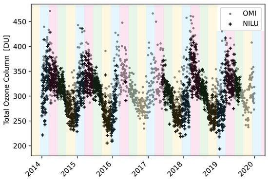
Figure 8.
The seasonal variations in TOC amounts: blue: winter, pink: spring, green: summer, yellow: autumn.
The calculated annual and semi-annual variations are caused by seasonal changes in odd-oxygen production rates, temperature-dependent ozone destruction rates and transport by the mean circulation and by eddies [21].
Unfortunately, due to technical difficulties, after 2019, the availability of reliable NILU-UV data dropped significantly, but to create an up-to-date overview of the annual TOC amounts, the missing data points were replaced by data from OMI. The yearly TOC amounts are shown in Figure 9.
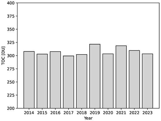
Figure 9.
Annual average TOC amounts from merged NILU-UV and OMI data for 2014–2023.
7.2. COD Results
As mentioned in Section 4, one output of the neural network is the cloud volume fraction, , which is converted to COD values at 380 nm, as shown in Figure 2. The results for the years 2014, 2015, 2018 and 2019 are shown in Figure 10a–d.
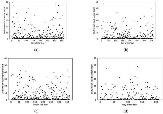
Figure 10.
Daily mean COD () values for (a) 2014, (b) 2015, (c) 2018 and (d) 2019.
The irradiance measurements of the 380 nm channel were used to derive the COD amounts, , because at this wavelength, there is negligible absorption by ozone and other trace gases (see Figure 7 in [12]). Thus, among the available channels, this channel is responsive to clouds but has the smallest sensitivity to ozone. The maximum daily mean COD value observed in our study was 60, as shown in Figure 10, exceeding the maximum daily value of about 35 which was reported by Fan et al. (2014) [3].
Using a location-specific aerosol model described in [12], we found the estimated TOC amount error due to a heavy aerosol loading (i.e., due to an aerosol volume fraction of ) to be about 3 Dobson units. The main difference between the RMF value and the COD value () is that the RMF value, which is derived using a look-up table (LUT) method, is unreliable both under broken cloud conditions and for large surface albedo values [8]. Our MLNN-based method infers the COD value () simultaneously with the TOC amount and is therefore expected to give more reliable results than the LUT method, as was also argued by Fan et al. (2014) [3].
8. Conclusions
Our multi-layer neural network (MLNN) method that retrieves total ozone column (TOC) amounts and cloud optical depth (COD) values [i.e., ] simultaneously from NILU-UV measurements yields TOC amounts in close agreement with OMI retrievals. The percentage error estimates were similar to those presented in [3].
The neural network method described in [3] relies on the tuning of radial basis functions. Since such tuning is not needed in our MLNN method, it is more robust and easier to use. Also, in our MLNN method, the imperfect cosine response of the instrument is taken into account in the retrieval as described in Section 6. Overall, the two methodologies (MLNN and LUT) yielded similar results and error estimates as the OMI method (see Table 6).
In contrast to the LUT method, our MLNN approach accounts for cloud effects in the retrieval of TOC amounts. Even under heavily overcast conditions, up to , the retrieved TOC amounts were consistent and showed the same seasonal variation of ozone as the OMI measurements. To obtain acceptable TOC results from the NILU-UV measurements using the LUT method, one should require RMF , because if the RMF is less than 30, the cloud is deemed to be too optically thick for NILU-UV measurements to yield reliable TOC amounts using the LUT method. Our MLNN method provides a significant improvement in this regard as the MLNN results agree with the OMI results when data for which RMF were excluded.
The results in Figure 8 and Figure 9 show no significant change in the TOC amounts. The lowest annual TOC amount of 299.4 DU was found in 2017, and the highest annual average of TOC amount of 321.6 DU was found in 2019.
The error in the COD due to the presence of aerosols was found to be small (see Section 7.2). Beyond the previously discussed sources of error, the large footprint and low time resolution of OMI (once a day) contribute to the discrepancies between results obtained from the NILU-UV and OMI measurements. For the same reasons, the NILU-UV instrument is well suited for local short- or long-term monitoring of total ozone column (TOC) amounts, aerosol optical depth (AOD) values and cloud optical depth (COD) values.
Author Contributions
Conceptualization, M.S., W.L. and K.S.; Data curation, M.S.; Formal analysis, M.S.; Funding acquisition, K.S.; Investigation, M.S. and L.K.; Methodology, M.S. and W.L.; Project administration, K.S.; Resources, K.S.; Software, M.S. and W.L.; Supervision, W.L. and K.S.; Validation, M.S. and L.K.; Visualization, M.S.; Writing—original draft, M.S.; Writing—review and editing, J.J.S., T.S. and K.S. All authors have read and agreed to the published version of the manuscript.
Funding
This research received no external funding.
Institutional Review Board Statement
Not applicable.
Informed Consent Statement
Not applicable.
Data Availability Statement
The modeled synthetic data used for neural network training—the NILU-UV instrument files and raw measurement data—are provided along with the article. Due to the large volume of the satellite data files, all OMI data used in this study are publicly available from the NASA-GESDISC website [22].
Acknowledgments
We would like to acknowledge the Environmental Modeling Center (EMC) of the National Oceanic and Atmospheric Administration (NOAA)/National Weather Service (NWS)/National Centers for Environmental Prediction (NCEP)/for their support in the preparation of this manuscript.
Conflicts of Interest
The authors declare no conflicts of interest.
Abbreviations
The following abbreviations are used in this manuscript:
| APE | Absolute percent error |
| CCD | Charge-coupled device |
| COD | Cloud optical depth |
| DSA | Norwegian Radiation and Nuclear Safety Authority |
| EMC | Environmental Modeling Center |
| FWHM | Full width at half maximum |
| GESDISC | Goddard Earth Sciences Data and Information Services Center |
| LUT | Look-up table |
| MLNN | Multi-layer neural network |
| NASA | National Aeronautics and Space Administration |
| NCEP | National Centers for Environmental Prediction |
| NOAA | National Oceanic and Atmospheric Administration |
| NWS | National Weather Service |
| OMI | Ozone monitoring instrument |
| PE | Percent error |
| RBFNN | Radial basis function neural network |
| RMF | Radiation modification factor |
| RS | Recommended standard |
| SZA | Solar zenith angle |
| TOC | Total ozone column |
| UTC | Coordinated Universal Time |
| US | United States |
| USA | United States of America |
| UV | Ultraviolet |
Appendix A
The linear relationship attained between and (presented in Figure 2) is .
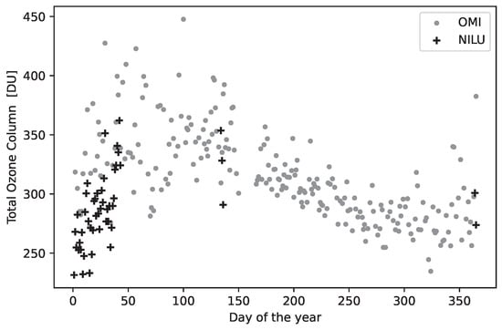
Figure A1.
TOC values from OMI (gray dots) and NILU-UV (black crosses) versus day of the year for 2016.
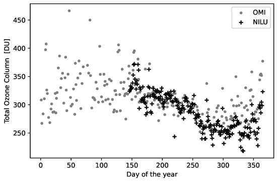
Figure A2.
TOC values from OMI (gray dots) and NILU-UV (black crosses) versus day of the year for 2017.
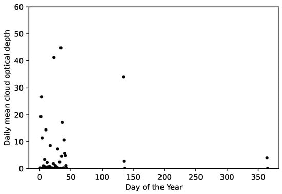
Figure A3.
Daily mean values versus day of the year for 2016.
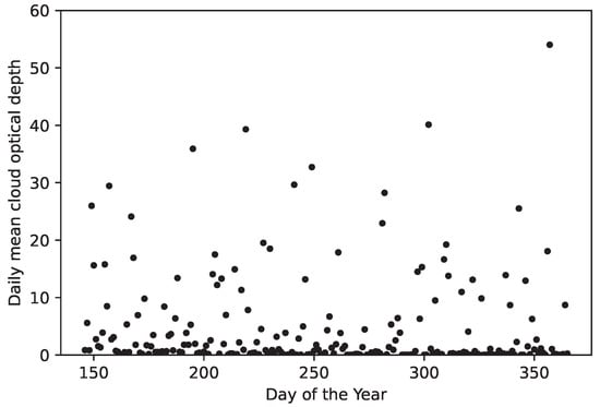
Figure A4.
Daily mean values versus day of the year for 2017.
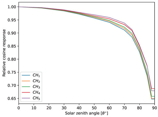
Figure A5.
The cosine response functions of the NILU-UV 115 instrument’s channels.
References
- Holick, M.F. Sunlight and vitamin D for bone health and prevention of autoimmune diseases, cancers, and cardiovascular disease. Am. J. Clin. Nutr. 2004, 80, 1678S–1688S. [Google Scholar] [CrossRef] [PubMed]
- Bishop, C.M.; Nasrabadi, N.M. Pattern Recognition and Machine Learning; Springer: Berlin/Heidelberg, Germany, 2006; Volume 4. [Google Scholar]
- Fan, L.; Li, W.; Dahlback, A.; Stamnes, J.J.; Stamnes, S.; Stamnes, K. New neural-network-based method to infer total ozone column amounts and cloud effects from multi-channel, moderate bandwidth filter instruments. Opt. Express 2014, 22, 19595–19609. [Google Scholar] [CrossRef] [PubMed]
- Stamnes, K.; Hamre, B.; Stamnes, S.; Chen, N.; Fan, Y.; Li, W.; Lin, Z.; Stamnes, J. Progress in Forward-Inverse Modeling Based on Radiative Transfer Tools for Coupled Atmosphere-Snow/Ice-Ocean Systems: A Review and Description of the AccuRT Model. Appl. Sci. 2018, 8, 2682. [Google Scholar] [CrossRef]
- Aalerud, T.N.; Johnsen, B. The Norwegian UV Monitoring Network; Norwegian Radiation Protection Authority: Østerås, Norway, 2006.
- Levelt, P.; van den Oord, G.; Dobber, M.; Malkki, A.; Visser, H.; de Vries, J.; Stammes, P.; Lundell, J.; Saari, H. The ozone monitoring instrument. IEEE Trans. Geosci. Remote Sens. 2006, 44, 1093–1101. [Google Scholar] [CrossRef]
- Sztipanov, M.; Tumeh, L.; Li, W.; Svendby, T.; Kylling, A.; Dahlback, A.; Stamnes, J.J.; Hansen, G.; Stamnes, K. Ground-based measurements of total ozone column amount with a multichannel moderate-bandwidth filter instrument at the Troll research station, Antarctica. Appl. Opt. 2020, 59, 97–106. [Google Scholar] [CrossRef] [PubMed]
- Høiskar, B.A.K.; Haugen, R.; Danielsen, T.; Kylling, A.; Edvardsen, K.; Dahlback, A.; Johnsen, B.; Blumthaler, M.; Schreder, J. Multichannel moderate-bandwidth filter instrument for measurement of the ozone-column amount, cloud transmittance, and ultraviolet dose rates. Appl. Opt. 2003, 42, 3472–3479. [Google Scholar] [CrossRef] [PubMed]
- The MathWorks Inc. MATLAB R2022b; The MathWorks Inc.: Natick, MA, USA, 2022. [Google Scholar]
- NASA; NOAA; USAF. U.S. Standard Atmosphere; U.S. Government Printing Office: Washington, DC, USA, 1976.
- Sugawara, H.; Takamura, T. Surface Albedo in Cities: Case Study in Sapporo and Tokyo, Japan. Bound.-Layer Meteorol. 2014, 153, 539–553. [Google Scholar] [CrossRef]
- Sztipanov, M.; Li, W.; Dahlback, A.; Stamnes, J.; Svendby, T.; Stamnes, K. Method for retrieval of aerosol optical depth from multichannel irradiance measurements. Opt. Express 2023, 31, 40070–40085. [Google Scholar] [CrossRef] [PubMed]
- Kazantzidis, A.; Bais, A.F.; Zempila, M.M.; Meleti, C.; Eleftheratos, K.; Zerefos, C.S. Evaluation of ozone column measurements over Greece with NILU-UV multi-channel radiometers. Int. J. Remote Sens. 2009, 30, 4273–4281. [Google Scholar] [CrossRef]
- LeCun, Y.; Bengio, Y.; Hinton, G. Deep learning. Nature 2015, 521, 436–444. [Google Scholar] [CrossRef] [PubMed]
- Pedregosa, F.; Varoquaux, G.; Gramfort, A.; Michel, V.; Thirion, B.; Grisel, O.; Blondel, M.; Prettenhofer, P.; Weiss, R.; Dubourg, V.; et al. Scikit-learn: Machine Learning in Python. J. Mach. Learn. Res. 2011, 12, 2825–2830. [Google Scholar]
- Kingma, D.P.; Ba, J. Adam: A method for stochastic optimization. arXiv 2014, arXiv:1412.6980. [Google Scholar]
- Broomhead, D.S.; Lowe, D. Radial Basis Functions, Multi-Variable Functional Interpolation and Adaptive Networks; Number 4148, Memorandum Report; Royal Signals and Radar Establishment: London, UK, 1988. [Google Scholar]
- Sztipanov, M. Methods for Retrieval of Ozone Amount, Cloud and Aerosol Optical Depth from Ground-Based Irradiance Measurements. Ph.D. Thesis, Stevens Institute of Technology, Hoboken, NJ, USA, 2023. [Google Scholar]
- Hastie, T.; Tibshirani, R.; Friedman, J. The Elements of Statistical Learning, 2nd ed.; Springer: New York, NY, USA, 2017. [Google Scholar]
- Dahlback, A. Measurements of biologically effective UV doses, total ozone abundances, and cloud effects with multichannel, moderate bandwidth filter instruments. Appl. Opt. 1996, 35, 6514–6521. [Google Scholar] [CrossRef] [PubMed]
- Perliski, L.M.; Solomon, S.; London, J. On the interpretation of seasonal variations of stratospheric ozone. Planet. Space Sci. 1989, 37, 1527–1538. [Google Scholar] [CrossRef]
- NASA. Goddard Earth Sciences Data and Information Services Center. Available online: https://disc.gsfc.nasa.gov (accessed on 23 January 2024).
Disclaimer/Publisher’s Note: The statements, opinions and data contained in all publications are solely those of the individual author(s) and contributor(s) and not of MDPI and/or the editor(s). MDPI and/or the editor(s) disclaim responsibility for any injury to people or property resulting from any ideas, methods, instructions or products referred to in the content. |
© 2024 by the authors. Licensee MDPI, Basel, Switzerland. This article is an open access article distributed under the terms and conditions of the Creative Commons Attribution (CC BY) license (https://creativecommons.org/licenses/by/4.0/).