Sea Fog Recognition near Coastline Using Millimeter-Wave Radar Based on Machine Learning

Abstract

Sea fog is a hazardous natural phenomenon that reduces visibility, posing a threat to ports and nearshore navigation, making the identification of nearshore sea fog crucial. Millimeter-wave radar has significant advantages over satellites in capturing sudden and localized sea fog weather. The use of millimeter-wave radar for sea fog identification is still in the exploratory stage in operational fields. Therefore, this paper proposes a nearshore sea fog identification algorithm that combines millimeter-wave radar with multiple machine learning methods. Firstly, Density-Based Spatial Clustering of Applications with Noise (DBSCAN) is used to partition radar echoes, followed by the K-means clustering algorithm (KMEANS) to divide the partitions into recognition units. Then, Sea-Fog-Recognition-Convolutional Neural Network (SFRCNN) is used to classify whether the recognition units are sea fog areas, and finally, the partition coverage algorithm is employed to improve identification accuracy. The experiments conducted using millimeter-wave radar observation data from the Pingtan Meteorological Observation Base in Fujian, China, achieved an identification accuracy of 96.94%. The results indicate that the proposed algorithm performs well and expands the application prospects of such equipment in meteorological operations.

1. Introduction

Sea fog is an important meteorological phenomenon, similar to wind and precipitation. It is also known as marine fog and usually occurs in the lower atmosphere over the ocean surfaces or coastal areas, where horizontal visibility is reduced to less than 1 km due to a large accumulation of water droplets or ice crystals (or both) [1,2]. Sea fog adversely affects transportation, fishery farming, oil and gas exploration and development, and marine social and economic activities due to its greatly reduced visibility. In particular, poor visibility caused by sea fog is a major contributor to ship collisions, posing a serious threat to life and property in maritime navigation. Sea fog is a catastrophic weather phenomenon, and sea fog identification is absolutely meaningful work that can help to reduce losses and avoid risks [3,4,5].

Satellite remote sensing technology is one of the primary tools for sea fog monitoring. Compared to ground observations, it is good at providing more real-time, accurate, and wider coverage of sea fog information [6,7]. Scientists utilize satellite remote sensing data, comprehensively employing techniques such as spectral analysis and structural analysis. By analyzing the spectral characteristics of each satellite channel, they extract the characteristic differences of sea fog reflected in the remote sensing data, thus conducting sea fog monitoring and applications, achieving significant results [8,9,10,11]. Han et al. [12] conducted sea fog monitoring using the reflectivity difference between fog and other objects at 0.63 µm and the dual-channel difference method for both daytime and nighttime. Ryu et al. [13] proposed a sea fog detection algorithm based on Himawari-8 satellite data, utilizing the reflectance of visible and near-infrared bands (1.6 µm), which can be applied to optical satellites without shortwave infrared bands (3.9 µm). Wu et al. [14] developed an automatic sea fog monitoring algorithm based on Moderate Resolution Imaging Spectroradiometer data, incorporating multiple variables such as the normalized snow index and the normalized difference of near-infrared water vapor index.

However, with the continuous increase in the amount of remote sensing data and the complexity of data processing demands, the limitations of traditional methods have gradually become apparent. Machine learning methods, due to their ability to autonomously learn feature information from data, have seen sharply widespread application in remote sensing data analysis in recent years [15]. This approach not only enhances the efficiency and accuracy of data processing but also expands the application domains of remote sensing data. From image classification and object detection to change detection and semantic segmentation, the innovation and adaptability of machine learning have brought revolutionary advancements to the analysis and interpretation of remote sensing data [16,17,18,19,20,21,22].

Additionally, several exciting advancements for sea fog identification were exploited by previous research. For instance, Jeon et al. [23] utilized a transfer learning model to identify sea fog and verified the effects of different band combinations on sea fog identification. Zhou et al. [24] proposed a dual-branch sea fog detection network, which achieved comprehensive and accurate sea fog monitoring by incorporating sea fog events recorded by the Geostationary Ocean Color Imager (GOCI). Tang et al. [25] proposed a model based on a two-stage deep learning strategy. By using fully connected networks and convolutional neural networks, along with the established Yellow Sea and Bohai Sea fog datasets, they successfully enhanced the ability to distinguish between low clouds and sea fog in satellite images. Wang et al. [26] utilized FengYun-3D satellite images to detect sea fog by constructing a 13-dimensional feature matrix and using Cloud-Aerosol Lidar and Infrared Pathfinder Satellite Observation (CALIPSO) sample labels. They applied four supervised classification models: decision tree, support vector machine (SVM), k-nearest neighbors (KNN), and neural networks. The study results indicate that SVM, KNN, and neural networks show significant performance in distinguishing between sea fog and low-level clouds, but their effectiveness in detecting fog under cloud layers is relatively poor. Lu et al. [27] proposed an ECA-TransUnet model that combines convolutional neural networks (CNN) and transformers. By incorporating an efficient channel attention module and a dual-branch feedforward network module, this model effectively captures the global contextual information of sea fog data. The results indicate that this model significantly outperforms existing models that rely solely on CNNs. In summary, by utilizing methods such as transfer learning, deep learning, and supervised classification, these techniques have not only improved the efficiency and accuracy of data processing but also enhanced the ability to distinguish between sea fog and low clouds. These innovative approaches and models have brought revolutionary advancements to the analysis and interpretation of sea fog data.

Although machine learning has achieved remarkable results in sea fog identification and monitoring, there is still noteworthy room for improvement. Satellite monitoring of sea fog faces the following challenges: Firstly, interference from upper-level cloud systems makes all-weather real-time observation difficult, thereby affecting the effectiveness of satellite monitoring. Secondly, due to limitations in spatial and temporal resolution, satellites can only quantitatively monitor sea fog that has a long duration and a certain coverage area. However, there is a more urgent need to service sudden and localized sea fog events, which are often difficult for satellites to capture [28]. With the advancement of ground-based remote sensing technology, inspired by the application of meteorological radar in cloud and precipitation monitoring, experts hope to use millimeter-wave radar, which has a relatively shorter wavelength, for sea fog observation [29]. Uematsu et al. [30] conducted observational experiments using millimeter-wave radar to study the spatial distribution, intensity, formation, and dissipation characteristics of sea fog, and they performed a detailed analysis of the cellular structures observed in the radar echoes. Gultepe et al. [31] developed a physical model between atmospheric visibility and millimeter-wave radar observations through simulation and subsequently validated it in observational experiments. Boers et al. [32] analyzed the relationship between ground visibility and millimeter-wave radar reflectivity in radiation fog. They developed a droplet activation model using a Scanning Mobility Particle Sizer to analyze the spectral characteristics of fog droplets, highlighting that the chemical composition of the fog significantly influences the relationship between visibility and radar reflectivity.

To overcome the limitations of satellites in detecting sea fog, this research proposes a sea fog recognition algorithm based on machine learning using millimeter-wave radar. According to the authors’ knowledge, this study is the first to apply millimeter-wave radar to sea fog recognition, expanding its application in meteorological services. Utilizing millimeter-wave radar for nearshore sea fog recognition provides a feasible solution for nearshore sea fog detection and ensures safety for nearshore navigation. The main contributions of this study are as follows:

(1) Expanding the application of millimeter-wave radar data from classical cloud observation to nearshore sea fog detection and monitoring. This effectively leverages the advantages of rapid and efficient cloud radar observation, broadening the utilization scope of millimeter-wave radar data and extending its application range in meteorological operations.

(2) Addressing the challenges in the application of millimeter-wave radar data for sea fog recognition, the paper subdivides the recognition process into multiple steps, integrating various machine learning models. This approach establishes a novel sea fog recognition model based on cloud radar observational data, providing a new feasible method for the comprehensive application of millimeter-wave radar data in meteorological research and operations.

2. Materials and Methods

2.1. Data

This study conducted experiments using observation data from the scanning millimeter-wave radar installed at the Pingtan Meteorological Observation Base in Fujian. The radar is equipped with a fully solid-state transmitter, capable of three-dimensional scanning with an elevation angle range from −2° to 180° and an azimuth angle range from 0° to 360°, to obtain information on meteorological targets such as clouds, rain, and fog. The millimeter-wave radar employs two scanning modes: Plan Position Indicator (PPI) and Range Height Indicator (RHI). The parameters of the millimeter-wave radar are shown in

Table 1. Main parameters of millimeter-wave radar [29].

System	Parameter	Indicator
Antenna	Diameter/m	1.8
	Gain/dB	53
	Beam width/(°)	0.39
	Operating mode	Single transmit and receive
Transmitter	Frequency band	35 GHz ± 100 MHz
	Peak power/W	130
	Pulse width/μs	1, 5, 20
	Pulse repetition frequency/Hz	1000~10,000
Receiver	Linear dynamic range/dB	80
	Noise figure/dB	5.2
	Gain/dB	37.2
Final product	Reflectivity factor/dBz	−50~40
	Radial velocity/(m·s−1)	−17~17
	Velocity spectrum width/(m·s−1)	0~8
	Radial velocity ambiguity/dB	−30~5

.

Due to the elevation of the radar installation site being 23.5 m, the scanning process is significantly obstructed by ground objects. The data used in this study are from PPI scans with azimuth angles ranging from 10° to 190° (north is 0°), covering mostly sea surface areas. For instance, using PPI scans at a 1.5° elevation angle, considering the radar beam width and installation height, the lowest height of the detected echoes above sea level is approximately 50 m at 1 km, 154 m at 5 km, and 285 m at 10 km from the radar, all below the typical development height of sea fog. Therefore, this study uses PPI scan data at or below a 1.5° elevation angle and employs the reflectivity factor and velocity spectrum width from the PPI scan data as raw data for model training. The reflectivity factor is a physical quantity used to describe the strength of radar echoes and is commonly employed to describe the scattering effects of water droplets, raindrops, snowflakes, and other hydrometeors in the atmosphere. The velocity spectrum width refers to the width of the peak of the radar echo signal in the frequency domain and is typically used to describe the range of the velocity distribution of meteorological targets. The PPI scan data used in the experiment have a set of data at each integer azimuth angle, with a spatial resolution of 30 m and a data volume of 833. The scanning millimeter-wave radar at the Pingtan can collect up to 833 data points per azimuth angle.

The experimental data includes nine sea fog events observed in 2020 and 2021, which serve as the raw data for this study. Due to the lack of a standardized sea fog dataset, the data in this study were annotated by meteorological experts. In these nine sea fog events, a total of 82,920 samples were labeled, including 40,067 sea fog samples and 42,853 non-fog samples.

2.2. Methods

2.2.1. Data Partition

The data partition process is shown in Algorithm 1. The distance from the data point to the radar is assigned using the scale of the distance; if the data point is the R-th point on an angle, the distance from the point to the radar is R.

Algorithm 1: Data partition

Input: reflectivity factor of the data points (DZ), ϵ, MinPts, angular range of the sea surface data (AR) Output: data after partition

1:   add the angle (DA) and distance (R) of data points     2:   keep the data within the AR range; this experiment’s AR is between 10 degrees and 190 degrees     3:   select DA and R as partition attributes     4:   normalize the partitioned attributes     5:   delete data points for which no DZ exists, and the remaining points are considered as DP     6:   DBSCAN uses ϵ and MinPts as model parameters to cluster DP and complete data partitioning     7:   add partition labels

This study uses Density-Based Spatial Clustering of Applications with Noise (DBSCAN) [33] to group radar echo areas that are close and connected in space into the same connected domain. DBSCAN has two key parameters: radius (ϵ) and minimum number of points (MinPts). By adjusting these two parameters, we can optimize the division of connected domains. This paper selects suitable parameter values (ϵ = 0.1, MinPts = 10) through experiments to divide the connected domains.

2.2.2. Construction of Recognition Units

Given the actual occurrence of sea fog, sea fog areas generally appear in patches that are relatively independent of non-fog areas. As such, the algorithm’s recognition results for sea fog areas and non-fog areas should appear in patches, to avoid a mixture of small regions of different types. Based on the above considerations, the K-means clustering algorithm (KMEANS) [34] is used in this section to construct recognition units. The construction of recognition units is achieved by dividing each partition obtained in the data partitioning process into basic units, which can be used to divide sea fog areas and non-fog areas, to achieve the result that sea fog appears in continuous patches.

The area of the data points is shown in Equation (1), where R represents the distance of the data points, and S is a scale value as well as R. Equation (2) shows the area of the partition (Section 2.2.1 Data Partition). Here, $n$ represents the number of data points in the partition, $S_i$ represents the area corresponding to the i-th data point, and $SA$ is the total area of the partition. Equation (3) shows the calculation for the number of units in partition construction. Here, $SA$ stands for the area of the partition, $K$ is the number of units in partition construction, and K is the same as the value of $K$ in the KMEANS. The process of constructing the recognition unit is shown in Algorithm 2.

$$S=2\ast R-1$$

(1)

$$SA=\sum _{i=1}^n{S}_i$$

(2)

$$K=\lfloor SA/\mathrm{500,000}\rfloor +1$$

(3)

Algorithm 2: Construction of recognition units

Input: the set of partitions after data partition (P), reflectivity factor of data points (DZ) Output: data after constructing the recognition unit

1:  for P {     2:   use Equations (1) and (2) to calculate the partition area SA     3:   if SA < 500,000     4:     construct partition as single recognition unit, add recognition unit label     5:   else     6:     add the Cartesian coordinates (DC) of the data point     7:     select DZ and DC as constructed attributes     8:     normalize the constructed attribute,     9:     calculate K using Equation (3); the data point set within the partition is counted as PDP     10:    KMEANS uses K as a model parameter to cluster PDP and build recognition units     11:    add recognition unit labels     12: }

This study uses the KMEANS to divide the partition into appropriately sized recognition units. In KMEANS, the K value and the initial centroids are key parameters. The KMEANS is implemented using the scikit-learn software package (version 1.1.3) [35] with Python (version 3.8.19) [36]. In scikit-learn, KMEANS defaults to initializing 10 sets of different centroids and returns the best result to reduce errors from random initialization. Since the area of the recognition units is relatively stable, more recognition units need to be constructed when the partition area increases. Therefore, this research sets the number of recognition units (K value) to be positively related to the partition area. After experiments, this paper finds that the number of recognition units (K value) calculated by Equation (3) is reasonable.

2.2.3. Recognition Unit Classification

The recognition unit classification process is shown in Algorithm 3, and the preliminary recognition results are obtained after the recognition unit classification.

Algorithm 3: Recognition unit classification.

Input: set of partitions after data partition (P), reflectivity factor of the data points (DZ), Velocity spectrum width of data points (DW), SFRCNN Output: data after classification of recognition units

1:  for P {     2:    count the set PK of identified units in the partition     3:    for PK {     4:     select the classification attributes DZ and DW     5:     calculate the mean, standard deviation, minimum, 1/4 quantile, 2/4 quantile, 3/4 quantile, and maximum values of the categorical attributes in the recognition unit, remove the maximum value and standard deviation of DW, and record as DD_12     6:     after every 3 elements in DD_12, insert a data point with value 0 and reorganize it into 3-dimensional data of 1 × 4 × 4, denoted as DD_16     7:     DD_16 is input to SFRCNN to obtain the classification result     8:     classification result of marker recognition unit     9:    }     10: }

Neural networks are a subset of machine learning and are at the core of deep learning algorithms. The name and structure of neural networks are inspired by the human brain, as they mimic the way biological neurons signal and transmit information to each other. Artificial neural networks comprise layers of interconnected nodes, consisting of an input layer, one or more concealed layers, and an output layer. Each node, commonly referred to as an artificial neuron, is linked to another node using connected weights and thresholds. If the output of any individual node surpasses the designated threshold, the node is stimulated, and information is dispatched to the next layer of the network. Conversely, data will not advance to the subsequent layer of the network if the threshold is not exceeded.

The structure of the SFRCNN model is shown in Figure 1. The input data format is [1, 4, 4] ([Channels, Height, Width]; Channels, Height, and Width represent the different dimensions of the data). After 1 × 1 convolution, the number of channels becomes 2, and again after 1 × 1 convolution, the number of channels becomes 5. Then, after 2 × 2 maximum pooling and activation of the Rectified Linear Unit (RELU) and Flatten functions, the hidden layer has 20 nodes; furthermore, after two linear layers, the number of nodes becomes 2, and then the output is generated.

2.2.4. Partition Coverage

In the classification results of the recognition unit, there are two special cases: the first case is where most of the units in the partition are classified as non-fog, with only a few units classified as sea fog; the second case is where most of the units in the partition are sea fog, with only a few classified as non-fog. After experiments and expert analysis, we believe that when the two special cases mentioned occur, the phase with a smaller area in the partition is abnormal. In such cases, these abnormal phases should be covered by the phases with a larger area in the partition [37]. Therefore, this study proposes a partition coverage algorithm; the process is shown in Algorithm 4. In the algorithm, the expression for step 6 is: “((A/(A + B) > 0.35) and (B/(A + B) > 0.35) and (A > 6 × 10⁶) and (B > 6 × 10⁶)) or ((A > 2 × 10⁷) and (B > 2 × 10⁷))”. This expression is used to determine whether partitioning should be covered. Here, A represents the area of the fog region, and B represents the area of the non-fog region. The condition can be divided into two parts: the first part requires both A and B to be greater than 6 × 10⁶, and both A and B must each account for more than 35% of the total area; the second part requires both A and B to be greater than 2 × 10⁷. If either of these two conditions is met, partition coverage is not required; if neither condition is met, the partition coverage strategy will be adopted, meaning that larger areas will cover smaller areas. Based on experiments, this paper chose these reasonable thresholds. After partition coverage, the recognition results are more accurate.

Algorithm 4: Partition coverage

Input: the set of partitions after data partition (P) Output: data after partition coverage

1:  for P {     2:  if the classification results of all recognition units in the partition are uniform     3:    no partition coverage required     4:  else     5:    calculate the areas of the sea fog region (A) and the non-fog region (B) within the partition     6:    if ((A/(A + B) > 0.35) and (B/(A + B) > 0.35) and (A > 6 × 106) and (B > 6 × 106)) or ((A > 2 × 107) and (B > 2 × 107))     7:     no partition coverage required;     8:    else     9:     achieve partition coverage, where large areas cover small areas;     10: }

2.2.5. Evaluation Metrics

The three-fold cross-validation method was used for evaluation during the experiment. In each iteration, six sea fog events are selected as the training set for the model, and the remaining three are used as the test set. Finally, by averaging the results of each iteration, the validation results for the entire dataset are obtained. In this study, sea fog samples are considered positive samples, while non-fog samples are considered negative samples. We evaluate the model’s performance using accuracy (ACC), probability of detection (POD), and false alarm rate (FAR). ACC provides an overview of the overall model performance, measuring the model’s prediction accuracy across all samples (including both positive and negative classes). POD measures the model’s ability to identify positive samples, i.e., how well the model correctly identifies all positive samples. FAR measures the model’s false alarm rate for negative samples. All three metrics—ACC, POD, and FAR—range from 0 to 1, with an ideal ACC and POD score of 1 and an ideal FAR score of 0. In Equations (4)–(6), TP represents the true positive samples predicted by the model, FN represents the false negative samples predicted by the model, FP represents the false positive samples predicted by the model, and TN represents the true negative samples predicted by the model.

$$ACC={\displaystyle \frac{TP+TN}{TP+FP+TN+FN}}$$

(4)

$$POD={\displaystyle \frac{TP}{TP+FN}}$$

(5)

$$FAR={\displaystyle \frac{FP}{TP+FP}}$$

(6)

3. Results and Analysis

3.1. Sea Fog Recognition Experiment

The sea fog recognition experiment consists of Recognition Unit Classification (Section 2.2.3) and Partition Coverage (Section 2.2.4). By comparing the sea fog region and the non-fog region, it was found that there are differences in the reflectivity factor and velocity spectrum width between the two regions. In the experiment, the mean, standard deviation, minimum, 1/4 quantile, 2/4 quantile, 3/4 quantile, and maximum values of the reflectivity factor and spectral width of data points within the recognition unit were selected as the recognition unit classification attributes. The chi-square test [38,39,40] was next performed for selected attributes and partition categories. The results are shown in

Table 2. Chi-square test for the classification attribute of the recognition unit.

	p-Value
	Reflectivity Factor	Velocity Spectrum Width
Mean	1 × 10−6	0.001
Standard deviation	0.001	0.258
Minimum	1 × 10−6	0.008
1/4 quartile	1 × 10−6	0.018
2/4 quartile	1 × 10−6	0.005
3/4 quartile	1 × 10−6	0.001
Maximum	1 × 10−6	0.940

, and it can be found that the p-values of the standard deviation and the maximum value of the velocity spectrum width are greater than 0.05, so these two attributes are removed, and the remaining attributes are selected as the identification unit classification attributes.

In this paper, the experiment utilized Python (version 3.8.19) [36]. The models used are as follows: SVM [41], KNN [42], Gaussian Naive Bayes (GaussianNB) [43], and Logistic Regression (LR) [44] from scikit-learn (version 1.1.3) [35]; eXtreme Gradient Boosting (XGBoost) [45] from XGBoost library (XGB_Lib, version 2.0.3) [46]; and SFRCNN built with Pytorch (version 1.13.0) [47]. These algorithms represent different types of machine learning methods, including linear models, non-linear models, probabilistic models, and ensemble models, which are widely applied and demonstrate excellent performance. By comparing these algorithms, we can comprehensively evaluate the performance of the proposed algorithm.

We carefully tuned the model parameters using scikit-learn, XGB_Lib, and PyTorch to achieve optimal outcomes. The evaluation metrics for the test set in Recognition Unit Classification (Section 2.2.3) are shown in

Table 3. Recognition unit classification test set evaluation index table.

	ACC	POD	FAR
SVM	92.77%	93.15%	8.45%
KNN	92.63%	93.12%	8.68%
GaussianNB	92.65%	93.20%	8.72%
LR	93.09%	95.78%	9.91%
XGBoost	93.40%	96.42%	9.84%
SFRCNN	94.90%	97.59%	8.00%

. For Partition Coverage (Section 2.2.4), the test set evaluation metrics are presented in

Table 4. Sea fog recognition experiment test set evaluation index table.

	ACC	POD	FAR
SVM	94.74%	95.66%	6.73%
KNN	94.49%	95.40%	6.99%
GaussianNB	94.21%	95.28%	7.44%
LR	94.89%	97.66%	8.07%
XGBoost	94.93%	98.01%	8.27%
SFRCNN	96.94%	99.24%	5.50%

. Comparison between Table 3 and Table 4 reveals a significant improvement in classification performance metrics when using partitioning coverage, indicating that it is a reasonable and effective approach. In Table 4, SFRCNN performs best in terms of ACC, POD, and FAR metrics. Specifically, SFRCNN achieves an ACC of 96.94%, at least two percentage points higher than other methods; a POD of 99.24%, at least one percentage point higher than other methods; and an FAR of 5.5%, at least one percentage point lower than other methods. Therefore, we choose SFRCNN as the classifier for the sea fog recognition experiments.

3.2. Independent Test

To demonstrate the applicability of the algorithm proposed in this study, we selected three different cases for illustration and explanation, which are not included in the model’s training and testing datasets.

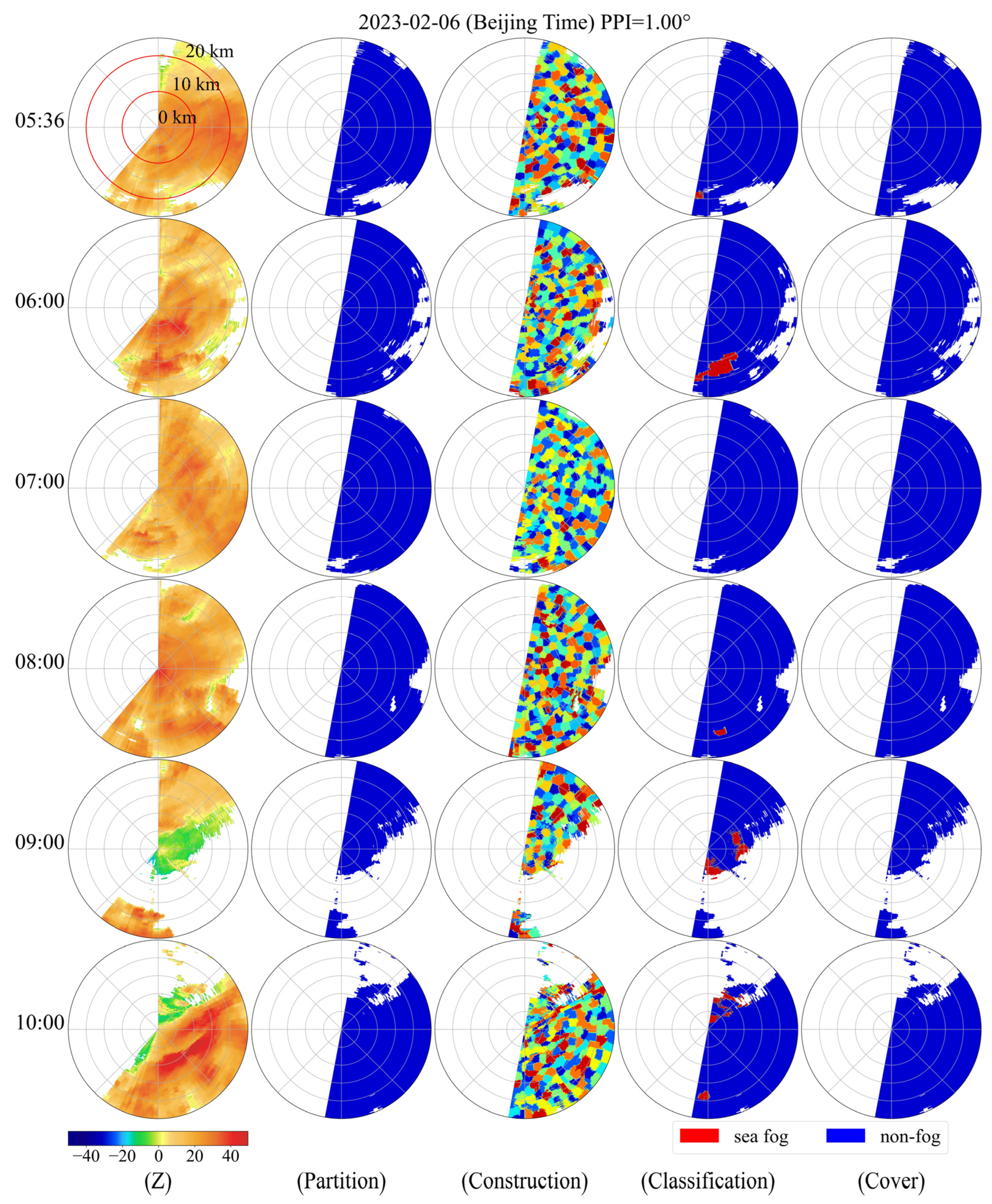
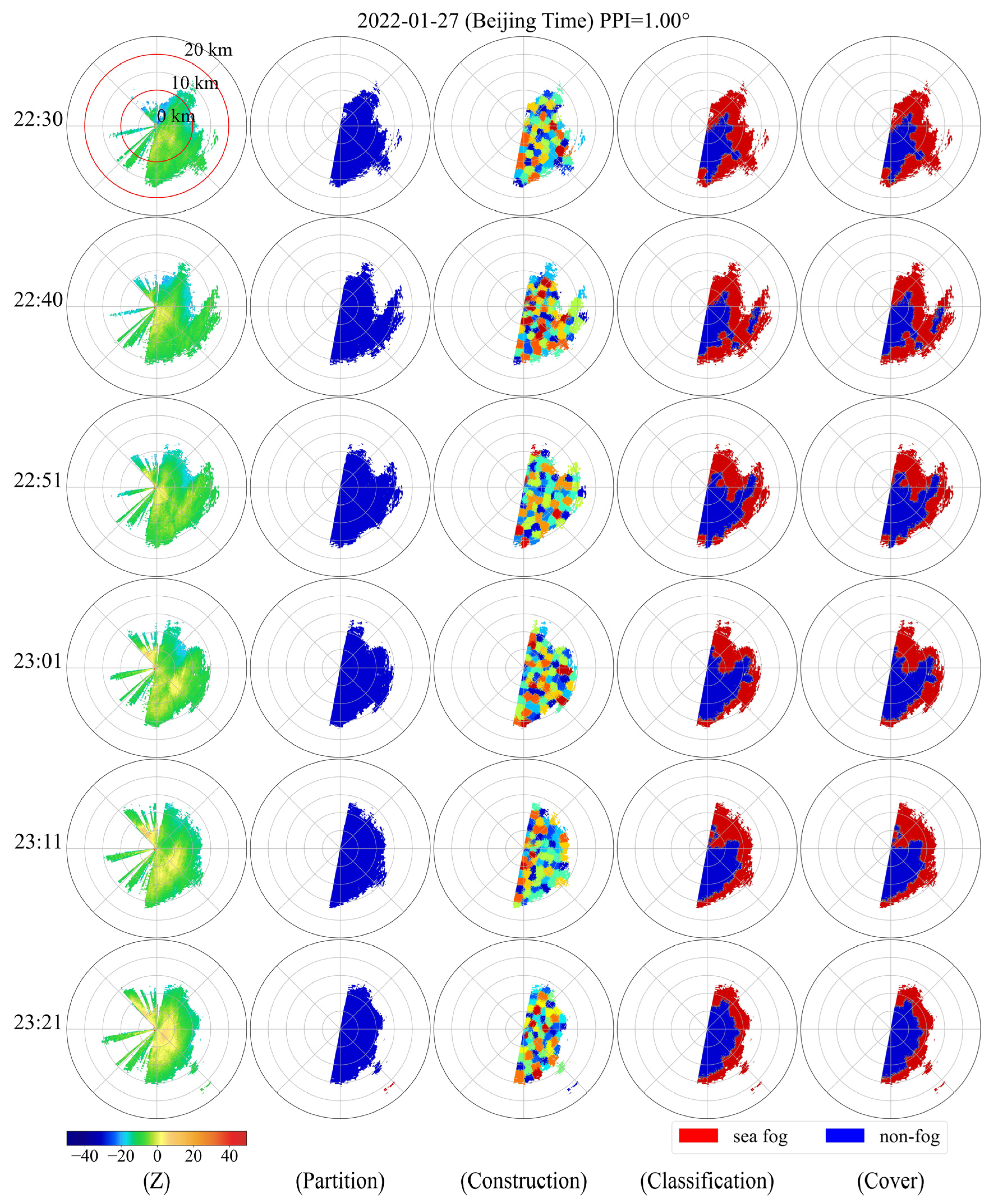
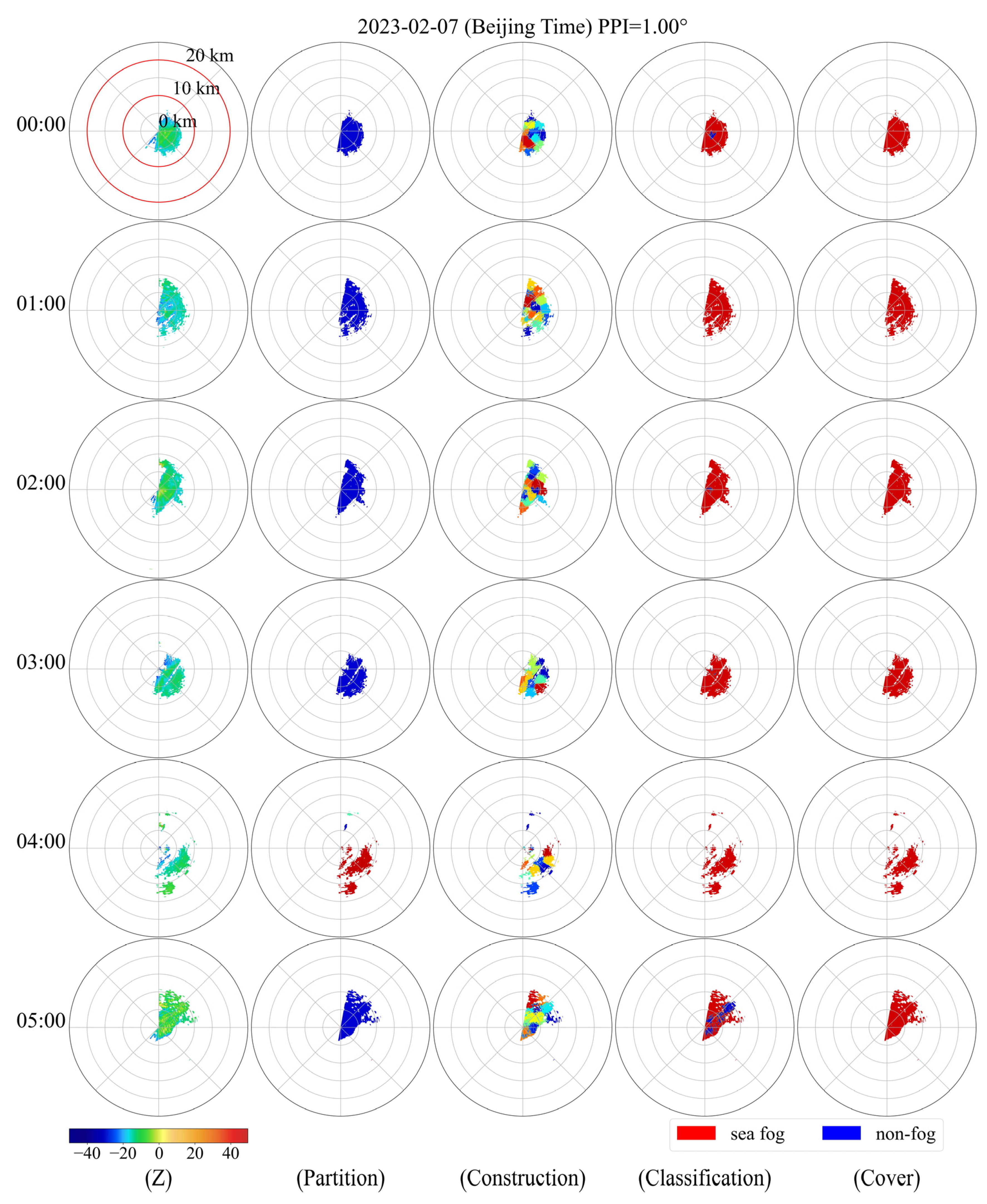
Case 1 (Figure 2): non-fog (precipitation) process. Case 2 (Figure 3): mixed rain and fog process. Case 3 (Figure 4): sea fog process. Figure 2, Figure 3 and Figure 4 (Z) display the radar reflectivity factor echo maps. Figure 2, Figure 3 and Figure 4 (Partition) present the partition results of the effective radar echo regions, with different colors representing different partitions. Figure 2, Figure 3 and Figure 4 (Construction) show the partition identification units, with different colors indicating different identification units. Figure 2, Figure 3 and Figure 4 (Classification) display the classification results of the identification units, where red indicates sea fog regions and blue indicates non-fog regions. Figure 2, Figure 3 and Figure 4 (Cover) present the classification results after applying the coverage method, where red indicates sea fog regions and blue indicates non-fog regions.

Case 1: Figure 2 shows the performance of our algorithm in non-fog conditions. Ideally, all areas should be correctly identified as non-fog regions. In Figure 2 (Classification), most non-fog areas are accurately recognized. However, a few non-fog areas are mistakenly identified as sea fog areas. To address this, we proposed Algorithm 4 (Partition Coverage). Using Algorithm 4 on the results from Figure 2 (Classification), we find that it meets the partition coverage requirement. Here, the non-fog area is larger than the sea fog area, so the non-fog area covers the sea fog area. Therefore, in Figure 2 (Cover), the blue area covers the red area, achieving the ideal result.

Case 2: Figure 3 shows the performance in mixed conditions. In this case, the center area is non-fog, and the outer area is sea fog. The difference from Figure 2 is that Algorithm 4 does not perform partition coverage. Therefore, in Figure 4 (Cover), the center area is non-fog, and the outer area is sea fog. This indicates that the identification result effectively distinguishes between sea fog and non-fog.

Case 3: Figure 4 shows the performance of our algorithm in sea fog conditions. Ideally, all areas should be correctly identified as sea fog regions. The difference from Figure 2 is that after applying Algorithm 4, the sea fog area covers the non-fog area. Therefore, in Figure 4 (Cover), the red area covers the blue area, achieving the ideal result.

Cases 1–3 demonstrate the high feasibility of our method for identifying both single and mixed conditions.

4. Conclusions

This paper proposes a nearshore sea fog identification algorithm that combines millimeter-wave radar and multiple machine learning methods. The algorithm aims to explore the application of millimeter-wave radar in nearshore sea fog detection. It extends the functionality of millimeter-wave radar from cloud detection to sea fog detection, thereby enhancing the device’s applicability. Compared to satellites and other detection devices, millimeter-wave cloud radar offers higher spatial and temporal resolution, making it more suitable for detecting localized nearshore sea fog. The algorithm first uses DBSCAN to partition radar echoes, then applies KMEANS to segment these partitions into recognition units. Subsequently, SFRCNN is employed to classify the recognition units, and finally, a partition coverage algorithm is used to improve identification accuracy. In the test set, the algorithm achieved an ACC of 96.94%, a POD of 99.24%, and an FAR of 5.5%. Additionally, the algorithm was validated through three independent processes in different states, further confirming its effectiveness in distinguishing between fog and non-fog areas. Thus, the proposed algorithm effectively addresses the problem of nearshore sea fog detection, providing reliable safety assurance for nearshore navigation. Additionally, it expands the application prospects of millimeter-wave radar in meteorological services. However, millimeter-wave radar in sea fog research is still in its infancy, and further exploration is needed in several areas in the future. For instance, developing more advanced data annotation methods and conducting research on the inversion of fog visibility.

References

1. Bendix, J. A satellite-based climatology of fog and low-level stratus in Germany and adjacent areas. Atmos. Res. 2002, 64, 3–18. [Google Scholar] [CrossRef]
2. Gultepe, I.; Tardif, R.; Michaelides, S.C.; Cermak, J.; Bott, A.; Bendix, J.; Müller, M.D.; Pagowski, M.; Hansen, B.; Ellrod, G. Fog research: A review of past achievements and future perspectives. Pure Appl. Geophys. 2007, 164, 1121–1159. [Google Scholar] [CrossRef]
3. Akimoto, Y.; Kusaka, H. A climatological study of fog in Japan based on event data. Atmos. Res. 2015, 151, 200–211. [Google Scholar] [CrossRef]
4. Guo, J.; Li, P.; Fu, G.; Zhang, W.; Gao, S.; Zhang, S. The structure and formation mechanism of a sea fog event over the Yellow Sea. J. Ocean Univ. 2015, 14, 27–37. [Google Scholar] [CrossRef]
5. Yi, L.; Thies, B.; Zhang, S.; Shi, X.; Bendix, J. Optical thickness and effective radius retrievals of low stratus and fog from MTSAT daytime data as a prerequisite for Yellow Sea fog detection. Remote Sens. 2015, 8, 8. [Google Scholar] [CrossRef]
6. Mahdavi, S.; Amani, M.; Bullock, T.; Beale, S. A probability-based daytime algorithm for sea fog detection using GOES-16 imagery. IEEE J. Sel. Top. Appl. Earth Observ. Remote Sens. 2020, 14, 1363–1373. [Google Scholar] [CrossRef]
7. Du, P.; Zeng, Z.; Zhang, J.; Liu, L.; Yang, J.; Qu, C.; Jiang, L.; Liu, S. Fog season risk assessment for maritime transportation systems exploiting Himawari-8 data: A case study in Bohai Sea, China. Remote Sens. 2021, 13, 3530. [Google Scholar] [CrossRef]
8. Ahn, M.; Sohn, E.; Hwang, B. A new algorithm for sea fog/stratus detection using GMS-5 IR data. Adv. Atmos. Sci. 2003, 20, 899–913. [Google Scholar] [CrossRef]
9. Fu, G.; Guo, J.; Pendergrass, A.; Li, P. An analysis and modeling study of a sea fog event over the Yellow and Bohai Seas. J. Ocean Univ. 2008, 7, 27–34. [Google Scholar] [CrossRef]
10. Zhang, S.; Yi, L. A comprehensive dynamic threshold algorithm for daytime sea fog retrieval over the Chinese adjacent seas. Pure Appl. Geophys. 2013, 170, 1931–1944. [Google Scholar] [CrossRef]
11. Yang, J.; Yoo, J.; Choi, Y. Advanced dual-satellite method for detection of low stratus and fog near Japan at dawn from FY-4A and Himawari-8. Remote Sens. 2021, 13, 1042. [Google Scholar] [CrossRef]
12. Han, J.; Suh, M.; Yu, H.; Roh, N. Development of fog detection algorithm using GK2A/AMI and ground data. Remote Sens. 2020, 12, 3181. [Google Scholar] [CrossRef]
13. Ryu, H.; Hong, S. Sea fog detection based on Normalized Difference Snow Index using advanced Himawari imager observations. Remote Sens. 2020, 12, 1521. [Google Scholar] [CrossRef]
14. Wu, X.; Li, S. Automatic sea fog detection over Chinese adjacent oceans using Terra/MODIS data. Int. J. Remote Sens. 2014, 35, 7430–7457. [Google Scholar] [CrossRef]
15. Lecun, Y.; Bengio, Y.; Hinton, G. Deep learning. Nature 2015, 521, 436–444. [Google Scholar] [CrossRef]
16. Hirahara, N.; Sonogashira, M.; Iiyama, M. Cloud-free sea-surface-temperature image reconstruction from anomaly inpainting network. IEEE Trans. Geosci. Remote Sens. 2021, 60, 4203811. [Google Scholar] [CrossRef]
17. Jing, Y.; Lin, L.; Li, X.; Li, T.; Shen, H. Cascaded downscaling–calibration networks for satellite precipitation estimation. IEEE Geosci. Remote Sens. Lett. 2022, 19, 1506105. [Google Scholar] [CrossRef]
18. Zhu, S.; Wang, X.; Jiao, D.; Zhang, Y.; Liu, J. Spatial Downscaling of GPM Satellite Precipitation Data Using Extreme Random Trees. Atmosphere 2023, 14, 1489. [Google Scholar] [CrossRef]
19. Sachindra, D.A.; Ahmed, K.; Rashid, M.M.; Shahid, S.; Perera, B. Statistical downscaling of precipitation using machine learning techniques. Atmos. Res. 2018, 212, 240–258. [Google Scholar] [CrossRef]
20. Jing, Y.; Lin, L.; Li, X.; Li, T.; Shen, H. An attention mechanism based convolutional network for satellite precipitation downscaling over China. J. Hydrol. 2022, 613, 128388. [Google Scholar] [CrossRef]
21. Glawion, L.; Polz, J.; Kunstmann, H.; Fersch, B.; Chwala, C. spateGAN: Spatio-temporal downscaling of rainfall fields using a cGAN approach. Earth Space Sci. 2023, 10, e2023EA002906. [Google Scholar] [CrossRef]
22. Sha, Y.; Gagne Ii, D.J.; West, G.; Stull, R. Deep-learning-based gridded downscaling of surface meteorological variables in complex terrain. Part II: Daily precipitation. J. Appl. Meteorol. Climatol. 2020, 59, 2075–2092. [Google Scholar] [CrossRef]
23. Jeon, H.; Kim, S.; Edwin, J.; Yang, C. Sea fog identification from GOCI images using CNN transfer learning models. Electronics 2020, 9, 311. [Google Scholar] [CrossRef]
24. Zhou, Y.; Chen, K.; Li, X. Dual-branch neural network for sea fog detection in geostationary ocean color imager. IEEE Trans. Geosci. Remote Sens. 2022, 60, 4208617. [Google Scholar] [CrossRef]
25. Tang, Y.; Yang, P.; Zhou, Z.; Zhao, X. Daytime Sea Fog Detection Based on a Two-Stage Neural Network. Remote Sens. 2022, 14, 5570. [Google Scholar] [CrossRef]
26. Wang, Y.; Qiu, Z.; Zhao, D.; Ali, M.A.; Hu, C.; Zhang, Y.; Liao, K. Automatic detection of daytime sea fog based on supervised classification techniques for fy-3d satellite. Remote Sens. 2023, 15, 2283. [Google Scholar] [CrossRef]
27. Lu, H.; Ma, Y.; Zhang, S.; Yu, X.; Zhang, J. Daytime Sea Fog Identification Based on Multi-Satellite Information and the ECA-TransUnet Model. Remote Sens. 2023, 15, 3949. [Google Scholar] [CrossRef]
28. Hu, S.Z.; Wang, Z.C.; Zhang, X.F.; Tao, F.; Ding, H.X.; Li, C.N. Analysis of Sea Fog Echo Characteristics and Visibility Inversion of Millimeter-Wave Radar. Meteor Mon. 2022, 48, 1270–1280. [Google Scholar]
29. Hu, S.Z.; Cao, X.Z.; Tao, F.; Zhang, X.F. Comparative Analysis of Cloud Macro Characteristics from Two ShipbornedMillimeter Wave Cloud Radars in the West Pacific. Meteor Mon. 2020, 46, 745–752. [Google Scholar]
30. Uematsu, A.; Hashiguchi, H.; Teshiba, M.; Tanaka, H.; Hirashima, K.; Fukao, S. Moving cellular structure of fog echoes obtained with a millimeter-wave scanning Doppler radar at Kushiro, Japan. J. Appl. Meteorol. Climatol. 2005, 44, 1260–1273. [Google Scholar] [CrossRef]
31. Gultepe, I.; Pearson, G.; Milbrandt, J.A.; Hansen, B.; Platnick, S.; Taylor, P.; Gordon, M.; Oakley, J.P.; Cober, S.G. The fog remote sensing and modeling field project. Bull. Amer. Meteorol. Soc. 2009, 90, 341–360. [Google Scholar] [CrossRef]
32. Boers, R.; Baltink, H.K.; Hemink, H.J.; Bosveld, F.C.; Moerman, M. Ground-based observations and modeling of the visibility and radar reflectivity in a radiation fog layer. J. Atmos. Ocean. Technol. 2013, 30, 288–300. [Google Scholar] [CrossRef]
33. Ester, M.; Kriegel, H.; Sander, J.; Xu, X. A density-based algorithm for discovering clusters in large spatial databases with noise. In Kdd; University of Munich: München, Germany, 1996; pp. 226–231. [Google Scholar]
34. Krishna, K.; Murty, M.N. Genetic K-means algorithm. IEEE Trans. Syst. Man Cybern. Part B Cybern. 1999, 29, 433–439. [Google Scholar] [CrossRef] [PubMed]
35. Scikit-Learn. Available online: https://scikit-learn.org/stable/auto_examples/release_highlights/plot_release_highlights_1_1_0.html (accessed on 16 August 2024).
36. Python. Available online: https://www.python.org/ (accessed on 16 August 2024).
37. Bringi, V.N.; Chandrasekar, V. Polarimetric Doppler Weather Radar: Principles and Applications; Cambridge University Press: Cambridge, UK, 2001. [Google Scholar]
38. Pearson, K.X. On the criterion that a given system of deviations from the probable in the case of a correlated system of variables is such that it can be reasonably supposed to have arisen from random sampling. Lond. Edinb. Dublin Philos. Mag. J. Sci. 1900, 50, 157–175. [Google Scholar] [CrossRef]
39. Fisher, R.A. On the interpretation of χ2 from contingency tables, and the calculation of P. J. R. Stat. Soc. 1922, 85, 87–94. [Google Scholar] [CrossRef]
40. Cochran, W.G. The χ2 test of goodness of fit. Ann. Math. Stat. 1952, 23, 315–345. [Google Scholar] [CrossRef]
41. Cortes, C.; Vapnik, V. Support-vector networks. Mach. Learn. 1995, 20, 273–297. [Google Scholar] [CrossRef]
42. Cover, T.; Hart, P. Nearest neighbor pattern classification. IEEE Trans. Inf. Theory 1967, 13, 21–27. [Google Scholar] [CrossRef]
43. Zhang, H. The optimality of naive Bayes. Aa 2004, 1, 3. [Google Scholar]
44. Cox, D.R. The regression analysis of binary sequences. J. R. Stat. Soc. Ser. B Stat. Methodol. 1958, 20, 215–232. [Google Scholar] [CrossRef]
45. Chen, T.; Guestrin, C. Xgboost: A scalable tree boosting system. In Proceedings of the 22nd ACM Sigkdd International Conference on Knowledge Discovery and Data Mining, San Francisco, CA, USA, 13–17 August 2016; pp. 785–794. [Google Scholar]
46. XGBoost. Available online: https://xgboost.readthedocs.io/en/release_2.0.0/python/python_intro.html (accessed on 16 August 2024).
47. Pytorch. Available online: https://pytorch.org/get-started/previous-versions/ (accessed on 16 August 2024).
Figure 1. SFRCNN model structure. The input data format is [1, 4, 4] ([Channels, Height, Width]). After the first Conv2d, the data format changes to [2, 4, 4]. Then, after the second Conv2d, the format changes to [5, 4, 4]. Next, after the MaxPool2d, the data format changes to [5, 2, 2]. After the ReLU and Flatten, the data are transformed into a linear form with 20 nodes. Finally, after two Linear, the number of nodes is reduced to 2, and the output is produced.
Atmosphere 15 01031 g001
Figure 2. Case of the non-fog process. In this process, all areas are non-fog areas. In the final result (Cover), all areas are shown in blue (non-fog), which indicates that the identification result is correct. (Z) is the echogram of the reflectivity factor. (Partition) represents data partition. (Construction) represents the construction of recognition units. (Classification) represents recognition unit classification. (Cover) represents partition coverage. The red areas in (Classification) and (Cover) are sea fog areas, and the blue areas are non-fog areas. In the upper left subplot, the center of the subplot represents the starting point (0 km), with each circle’s distance from the center increasing by 5 km. The first red circle close to the center indicates 10 km away from the center, while the second red circle far from the center indicates 20 km away from the center.
Atmosphere 15 01031 g002
Figure 3. Case of the mixed process. In this process, the center area is non-fog, and the outer area is sea fog. In the final result (Cover), the center area is shown in blue (non-fog), and the outer area is shown in red (sea fog). This indicates that the identification result effectively distinguishes between sea fog and non-fog. (Z) is the echogram of the reflectivity factor. (Partition) represents data partition. (Construction) represents the construction of recognition units. (Classification) represents recognition unit classification. (Cover) represents partition coverage. The red areas in (Classification) and (Cover) are sea fog areas, and the blue areas are non-fog areas. In the upper left subplot, the center of the subplot represents the starting point (0 km), with each circle’s distance from the center increasing by 5 km. The first red circle close to the center indicates 10 km away from the center, while the second red circle far from the center indicates 20 km away from the center.
Atmosphere 15 01031 g003
Figure 4. Case of the sea fog process. In this process, all areas are sea fog areas. In the final result (Cover), all areas are shown in red (sea fog), which indicates that the identification result is correct. (Z) is the echogram of the reflectivity factor. (Partition) represents data partition. (Construction) represents the construction of recognition units. (Classification) represents recognition unit classification. (Cover) represents partition coverage. The red areas in (Classification) and (Cover) are sea fog areas, and the blue areas are non-fog areas. In the upper left subplot, the center of the subplot represents the starting point (0 km), with each circle’s distance from the center increasing by 5 km. The first red circle close to the center indicates 10 km away from the center, while the second red circle far from the center indicates 20 km away from the center.
Atmosphere 15 01031 g004