Abstract
How to decouple economic growth from carbon dioxide emissions and achieve low-carbon transformation of the Chinese economy has become an urgent problem that needs to be solved. Firstly, the Tapio index is used to identify China’s carbon peak status, and then the Technology Choice Index (TCI) and economic complexity are introduced into the comprehensive factor analysis framework for carbon dioxide emissions. Key influencing factors are identified using random forest and ridge regression. On this basis, a novel sparrow search algorithm–long short-term memory (SSA-LSTM) model which has more prediction accuracy compared with past studies is constructed to predict the dynamic evolution trend of carbon dioxide emissions, and in combination with scenario analysis, the path towards the carbon peak is simulated. The following conclusions are obtained: The benchmark scenario peaks in 2031, with a peak of 12.346 billion tons, and the low-carbon scenario peaks in 2030, with a peak of 11.962 billion tons. The extensive scenario peaks in 2037, with a peak of 13.291 billion tons. Under six scenarios, it can be concluded that energy intensity is the key factor in reducing the peak. These research results provide theoretical support for decision-makers to formulate emission reduction policies and adjust the carbon peak path.
1. Introduction
1.1. Research Background
Global climate change has led to frequent extreme weather events that are seriously affecting human sustainable development; carbon dioxide emissions have been identified as the main cause underlying global climate change [1]. According to IEA [2], as shown in Figure 1, China has surpassed the United States as the world’s largest carbon dioxide emitter since 2005. In 2021, China’s carbon dioxide emissions accounted for approximately 32.95% of the global total carbon dioxide emissions. Therefore, China is facing unprecedented pressure from a global warming perspective.
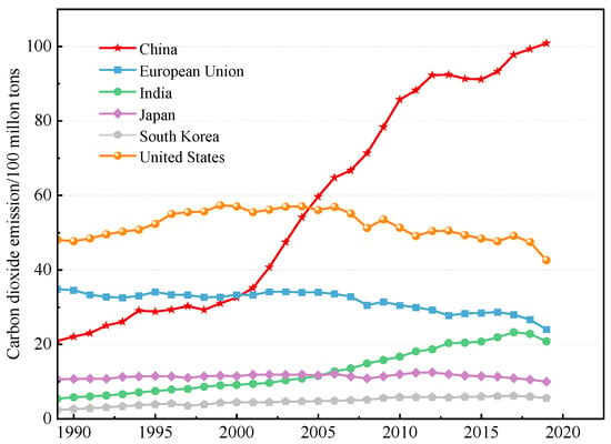
Figure 1.
Trends of carbon dioxide emissions in China, the USA, and other major economies.
To address climate change, China recently announced the new and long-term goals for its carbon dioxide emissions, stipulating the endeavor to achieve carbon peak by 2030 and carbon neutrality by 2060 [3]. The proposal of this dual carbon target indicates that China is increasingly attaching importance to environmental protection; China’s overall protection of the ecological environment will focus on carbon reduction in the future.
Without a doubt, the key issue is how a low-carbon transformation of China’s economy can be achieved. Because China’s industrial structure is currently still dominated by industry and its energy structure is dominated by coal [4], the steady growth of the Chinese economy relies on a considerable amount of fossil energy [5], which will lead to high carbon dioxide emissions. To achieve the dual carbon goal, China included a carbon dioxide emission indicator into the goals of the 14th Five Year Plan [6]. This plan stipulated that green and low-carbon development should be promoted, green transformation of industries should be advanced, energy resource allocation should be made more reasonable, and utilization efficiency should be significantly improved. In addition, according to the Action Plan for Carbon Peak before 2030 [7], China promised that by 2030, the proportion of non-fossil energy consumption will reach about 25%, and the carbon dioxide emissions per unit of Gross Domestic Product (GDP) will decrease by more than 60–65% compared to the 2005 level. This showcases China’s determination and confidence to reduce carbon dioxide emissions.
According to the above policy constraints, China urgently needs to implement relevant measures to control carbon dioxide emissions. Therefore, identifying the key influencing factors of carbon dioxide emissions, simulating the path towards carbon peak, and predicting the dynamic evolution trend are of central importance. In this paper, factors such as economy, population, urbanization rate, and energy consumption are constrained, and three paths towards carbon emission peak are simulated. This paper can provide relevant references for China’s carbon market quotas.
1.2. Literature Review
Research on carbon emission reduction is mainly divided according to the following two aspects: factors affecting carbon dioxide emissions and the prediction of carbon dioxide emissions. Clarifying the influencing factors and evolution trends of carbon dioxide emissions is important to achieve carbon peak. In this context, scholars chiefly discuss energy [8,9], industrial structure [10,11], economics [12,13], and technology [14], such as energy structure, energy intensity, GDP, industrial structure of various industries, urbanization rate, research and development funds, etc. The most common analysis models for analyzing influencing factors include LEAP [15], Kaya identity [16,17], the logarithmic mean Divisia index decomposition model [18], and the stochastic impacts by regression on population, affluence, and technology (STIRPAT) model [19]. The logarithmic mean Divisia index is decomposed based on Kaya’s identity and only considers a few factors, while the STIRPAT model features flexibility and randomness, and can analyze many influencing factors [20]. However, the above models have certain limitations, such as multicollinearity and sequence autocorrelation [21].
Therefore, machine learning models have recently been implemented in environmental research. By employing machine learning methods, various factors can be filtered to identify the key factors affecting carbon dioxide emissions. In accordance with the random forest model, Liu et al. [22] selected 56 factors and analyzed the dynamic transition of these factors. Qin et al. [23] applied the random forest model to select influencing factors, including socio-economic and environmental factors, and analyzed the effects of these factors on carbon dioxide emissions.
After identifying key factors, it makes logical sense to simulate the path towards carbon peak and reasonably predict the dynamic evolution trend of carbon dioxide emissions. Many models can be used for this, mainly including traditional econometric regression, machine learning, and deep learning models. Traditional econometric regression models, such as the common Kaya identity [24], IPAT model [25], and STIRPAT model [26,27,28], can be used to effectively analyze the relationship between influencing factors and carbon dioxide emissions. However, it is difficult to capture the nonlinear mapping dynamic relationship between influencing factors, and the prediction accuracy of these traditional models is not satisfactory [29]. Accordingly, machine learning and deep learning methods based on big data analysis achieve higher stability [23]. Scholars have established prediction models for carbon dioxide emissions based on machine learning, including support vector regression (SVR) [30], random forest [31], GA-SVR [32], back propagation (BP) [33,34], Lasso BP [35], Lasso-GRNN [36], and GA-LSTM [37]. The prediction of carbon peak is mainly based on time series data, and recurrent neural networks are an effective method for processing these data [38]. Long short-term memory (LSTM) networks, a special recurrent neural network model, can effectively solve problems of gradient vanishing and gradient explosion [38], thus they can obtain more accurate results. Therefore, based on the LSTM model, this paper innovatively establishes the sparrow search algorithm–long short-term memory (SSA-LSTM) model to predict the trend of China’s carbon dioxide emissions. Table 1 shows the methods used in the literatures.

Table 1.
Common analysis models and prediction models of CO2 emissions.
In summary, this paper provides a marginal contribution to the field of sustainable development according to the following three aspects: Firstly, the TCI and economic complexity are originally introduced from the field of development economics to the analysis framework of the comprehensive factors affecting carbon dioxide emissions. Secondly, random forest and ridge regression methods are selected to identify these influencing factors for analysis accuracy. Compared with traditional regression models, machine learning methods can consider as many carbon emission influencing factors as possible, thus avoiding the limitation of only selecting a few factors and ignoring other factors that may be important. Thirdly, the SSA is innovatively introduced to optimize the LSTM model, which is used to predict carbon dioxide emissions and simulate the path towards carbon peak by six different scenarios. The research presented in this paper provides reference for decision-makers to achieve China’s dual carbon goals and formulate reasonable policies.
1.3. Paper Structure
The paper mainly consists of the following parts: Section 1: The research background and current research status. Section 2: Introduction of the models used in this paper. Section 3: Results and Discussion. This chapter mainly includes data sources, decoupling analysis and simulation of the carbon peak path. This chapter first clarifies the current peak state in China. Then, we identify the key influencing factors of carbon dioxide emissions through random forest and ridge regression. Finally, we predict the carbon dioxide emissions though SSA-LSTM. Section 4: Conclusions.
2. Materials and Methods
2.1. Random Forest
If a large number of influencing factors are included in a predictive model, the accuracy of the prediction will be affected; therefore, a model needs to be selected to filter the factors that affect carbon dioxide emissions. Compared with traditional regression models, machine learning methods can consider many carbon emission influencing factors. Moreover, they offer the advantage of good robustness in processing massive data [22]. Therefore, this paper selects the random forest model to filter factors, and the importance of influencing factors is determined based on the Gini coefficient of random forest. Random forest based on decision tree is an algorithm that integrates multiple trees through ensemble learning [31]. If it is a classification problem, the voting result is obtained and the regression problem is solved using the average value. The random forest algorithm is shown as follows.
Assuming that there are C variables, namely, , , ,…, , its Gini coefficient is as follows [39]:
is the Gini coefficient of node m, where K represents the K categories in node m, and is the sample weight of category k in node m. Feature importance refers to the importance of feature at a node, which represents the change in the Gini coefficient before and after the node data are distributed to two sub nodes, which is represented as follows:
and represent the Gini exponents of two new nodes r and l, respectively, formed after node m is split. If the node of the variable in decision tree i is in the set M, the importance of the variable is calculated using the following formula:
The importance of variables in the forest of n trees is as follows:
Finally, the above importance is normalized to obtain the importance score of :
The importance of the influencing factor is evaluated by calculating the average decrease in the Gini index before and after node splitting. The larger the VIM value of the influencing factor, the more substantial its impact on carbon dioxide emissions; a small VIM value of a variable indicates that the impact on the dependent variable is not significant. Therefore, random forest can identify key factors affecting carbon dioxide emissions.
2.2. LSTM
The LSTM model is mainly used to process time series data. China’s carbon dioxide emissions have grown rapidly and experienced periodic fluctuations since 2010. The LSTM model can effectively digest this upward trend information and retain the long-term variation pattern of the sequence, thus making it very suitable to predict China’s carbon peak state [38]. Based on the evaluation indicators of predicted and true values, they are compared with several models and the model with the best prediction performance is selected for the prediction.
The main structure of the LSTM algorithm is as follows.
Input Gate: Control the flow of information into a storage unit and determine which information will be updated to the cell state using the sigmoid function [37]:
where W, U, and B are weights and errors, is the current signal input, is the previous input of the memory unit, and is a memory unit.
Forget Gate: Whether the information in the previous storage unit has accumulated at the current time is controlled and which old information should be forgotten is determined using the sigmoid function. The Forget Gate output is updated as follows:
Update Cell State: The cell state is updated by combining the results of the input gate and the forget gate. The new storage unit is updated as follows:
The results of LSTM structure nodes are output to output layer neurons:
Finally, the model needs to be tested for accuracy and error between actual and predicted values. This paper selects the mean absolute error (MAE), the mean squared error (MSE), the mean absolute percentage error (MAPE), and as testing metrics. The evaluation indicators used in this paper are as follows:
In the above evaluation indicators, and represent the predicted value of the model and the true value in the i-th sample, respectively. n represents the number of samples, and represents the average of the i-th sample. The range of R2 is [0–1], where the closer R2 is to 1, the better the prediction performance of the model. For MAPE, MAE, and MSE, the lower the indicator value, the higher the prediction accuracy. Based on the performance of the above evaluation indicators, the model with the best prediction performance is selected.
2.3. Sparrow Search Algorithm
SSA is an algorithm that is inspired by the group wisdom, foraging, and anti-predation behaviors of sparrows; it continuously updates the positions of discoverers and followers [40] and converges near the optimal value. A certain proportion of individuals will be selected from the population for examination and warning. If danger is identified, these individuals will choose to give up their food to ensure safety. Thus, this algorithm can find the optimal parameters for the model. This paper combines SSA with LSTM to accurately and quickly identify optimal parameters.
For sparrow populations [41],
n stands for the number of sparrows in the population, and d stands for the dimension attached to an individual sparrow.
The adaptability of sparrows is as follows:
During each iteration, the location of the discoverer is updated and described as follows:
where T is the maximum number of iterations; when the maximum number of iterations is reached, the model will stop running. is a random number, and and represent the warning value and safety value, respectively. is a random number subject to normal distribution, and L is a row vector with all elements of 1.
indicates that certain sparrows have identified danger. At this time, the discoverer should move to a safe position, i.e., the discoverer randomly moves to the current position according to a distribution. However, indicates that there is no danger in the current environment, and the discoverer can conduct a large-scale search operation. With increasing population algebra, the value range of the term will decrease, and the distribution of values will become more uniform, i.e., the values corresponding to each dimension of the sparrow body will decrease.
The updated location of the followers is as follows [42]:
where represents the worst position of the sparrow in the d dimension during the t iteration, and represents the optimal position of the sparrow in the d dimension at the t + 1 iteration of the population. A represents a row of the multidimensional matrix with each element being 1 or −1, , when indicates that the pursuer is in a very hungry state. The product of a standard normal distribution random number and exponential function with natural logarithm is used as the base to control its value to conform to a normal distribution, i.e., to obtain more energy.
In the sparrow population, the number of sparrows with an alert mechanism accounts for 10–20% of the total number, and their positions are randomly distributed. The position update formula is as follows:
where is the current global optimal position, represents the step size control parameter, and is a random number between [−1, 1], representing the direction of sparrow movement. represents the fitness value of the i-th sparrow, and and are the optimal and worst fitness values for the current sparrow population. When the sparrow is warned that it is currently in its optimal position, it will flee to a nearby location. If it is not in the optimal position, it will flee to the vicinity of the current optimal position until it finds the optimal position, thereby identifying a set of parameters to ensure optimal model performance.
3. Results and Discussion
3.1. Data Sources and Factors Affecting Carbon Dioxide Emissions
3.1.1. Data Sources
Considering the factors affecting carbon dioxide emissions studied in the existing literature, 26 representative influencing factors were selected from aspects such as economy, policy, environment, energy, industrial structure, population, and technology. The data were obtained from the “China Statistical Yearbook”, “China Environmental Statistical Yearbook”, “China Energy Statistical Yearbook”, “China Labor Statistics Yearbook”, the National Bureau of Statistics, the World Bank, and the Observatory of Economic Complexity Website. The data of carbon dioxide emissions from 1990 to 2019 were obtained from the China Emission Accounts and Datasets. The parameters for scenario setting refer to government planning documents and the relevant literature.
3.1.2. Factors Affecting Carbon Dioxide Emissions
Carbon dioxide emissions are affected by a variety of factors, including energy consumption, industrial structure, population and urbanization, and policies and technologies.
Energy consumption is one of the main factors affecting CO2 emissions. Numerous studies have shown that the consumption of fossil fuels, especially the use of coal, oil and natural gas, is a major source of CO2 emissions [8]. The industrial structure has a significant impact on CO2 emissions. Regions with a high proportion of heavy industry and energy-intensive industries also tend to have higher CO2 emissions [10]. Therefore, the adjustment of industrial structure is of great significance for reducing carbon emissions. Population growth and urbanization are also important factors influencing CO2 emissions [9]. As the population increases and the level of urbanization increases, the demand for energy is rising, which leads to an increase in CO2 emissions. Policy and technology developments play a key role in the control of carbon dioxide emissions. The government’s energy conservation and emission reduction policies, as well as the research and development and application of clean energy technologies, can effectively reduce carbon dioxide emissions [43].
Based on the factors of carbon dioxide emissions mentioned above, and in reference to the research of Liu [22], Qin et al. [23], and Lin [44], factors affecting carbon dioxide emissions can be selected from industrial structure, energy structure, economic growth, urbanization level, population, and environment. The TCI index from Lin Yifu’s new structural economics [44] and economic complexity [43] can be added to represent policy impact. In this paper, representative factors are selected from seven aspects; several factors are explained as follows.
- (1)
- Energy structure: Coal consumption accounts for the total energy consumption.
The TCI is used to measure the development strategy a country implements [44]:
and refer to the added value of the industry and the gross domestic product (GDP), respectively, of region i in year t. and refer to the number of employees in the industry and the total number of employed people, respectively, of region i in year t. and represent the average labor value added of the industry and the average labor GDP, respectively, of region i in year t, where represents the technology selection index of region i in year t. TCI indicates the direction of policies towards the industry.
- (2)
- Economic complexity: The data represent the correlation between industries. Policy stability can increase economic complexity [43] and is used to represent policy stability intensity.
- (3)
- Greenhouse gases: The website of the Organization for Economic Co-operation and Development specifies several greenhouse gases that impact climate change. In this paper, the impact of methane emissions on carbon dioxide emissions is selected.
- (4)
- Renewable energy generation: Renewable energies include hydropower, wind energy, solar energy, geothermal energy, and biomass energy; the data used in this paper do not include hydropower generation.
- (5)
- Air freight volume: The number of goods, express delivery, and diplomatic bags transported during each flight phase (from takeoff to next landing) are measured in metric tons multiplied by the number of kilometers flown. In this paper, this indicator is used to represent energy consumption during transportation.
To establish a more comprehensive indicator system of the factors influencing carbon dioxide emissions and to reflect the carbon dioxide emissions in more detail [22], in this paper, a system of factors from economy, policy, environment, energy, industrial structure, population, and technology is constructed. The 26 representative influencing factors selected in this paper and the data sources are shown in Table 2.

Table 2.
Influencing factors of carbon dioxide emissions.
3.2. Decoupling Analysis
Considering that the Tapio decoupling model can accurately reflect the situation between resources, environment, and economic growth in a region over a certain period of time, based on the Tapio values, this paper determines whether GDP and carbon dioxide emissions in the region are decoupled.
is the Tapio decoupling elastic coefficient. and are the differences in carbon dioxide emissions and GDP between two adjacent periods, respectively. e and g are the growth rate of carbon dioxide emissions and GDP, respectively [24].
According to the decoupling coefficient, this coefficient is divided into eight decoupling states. Strong decoupling refers to the situation where the economy is increasing and carbon dioxide emissions are decreasing, which is a good green economy development state. Strong negative decoupling refers to increasing carbon dioxide emissions and decreasing economy, which is the worst-case scenario; all other scenarios are in an intermediate state. To achieve the dual carbon goals, it is necessary to completely decouple GDP and carbon dioxide emissions. The eight decoupling states are shown in Figure 2.
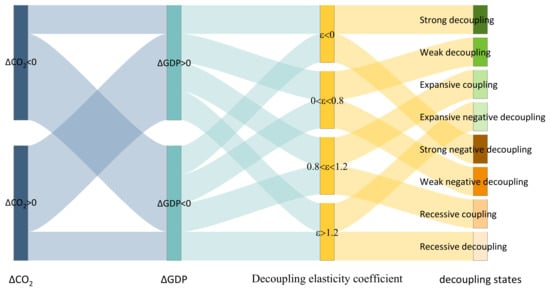
Figure 2.
Eight kinds of decoupling states.
According to the above formula, the Tapio decoupling elasticity coefficients of China from 1990 to 2019 are obtained, as shown in Table 3.

Table 3.
Tapio decoupling elasticity coefficients in China from 1990 to 2019.
Table 3 shows that in the decade from 1990 to 2000, China’s carbon dioxide emissions and GDP were in a state of strong and weak decoupling. However, during the “Tenth Five Year Plan” period, China was in a state of expansion coupling. Even in 2002–2003, the decoupling elasticity coefficient reached 1.26, indicating that the growth of carbon dioxide emissions exceeded the speed of economic growth at this time, which violated the requirements of green economy development.
With increasing national emission reduction efforts, the decoupling coefficient has started to decrease. Since 2005, the decoupling coefficient has followed a trend of first decreasing and then increasing. In 2014–2015, the decoupling elasticity coefficient was −0.21, indicating a strong decoupling state, while China was in a weak decoupling state at other times. In recent years, China’s economic growth has slowed down, and the decoupling elasticity coefficient has also shown a slight rebound. This indicates that China’s economic growth and carbon dioxide emissions will remain weakly decoupled for a period of time in the future. Because economic growth has not yet been completely decoupled from carbon dioxide emissions, relevant policy constraints are needed to achieve complete decoupling between economic growth and carbon dioxide emissions. Simultaneously, the future carbon peak situation needs to be studied to achieve stipulated carbon peak and carbon neutrality goals.
3.3. Simulating the Path towards Carbon Peak
3.3.1. Analysis and Screening of Factors Affecting Carbon Dioxide Emissions
Based on this paper’s selection of 26 influencing factors from the seven aspects of economy, industrial structure, energy, society, technology, policy, and environment (examples of which are the proportion of primary industry, TCI index, afforestation area, GDP, urbanization rate, foreign investment, energy intensity, energy structure, population, and sulfur dioxide emissions), the correlation coefficients between these influencing factors are calculated. Thus, the correlation coefficient matrix between them is obtained. This paper visualizes the correlation coefficient matrix and produces a thermodynamic diagram as shown in Figure 3.
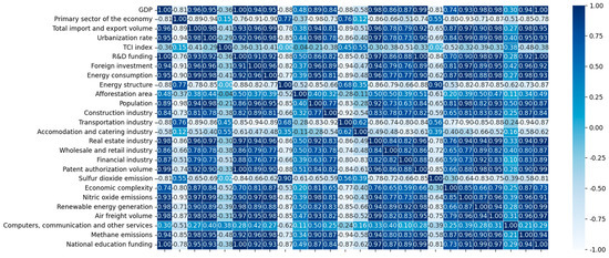
Figure 3.
Thermodynamic diagram of carbon dioxide emissions’ influencing factors.
Figure 3 clearly shows the linear relationship between influencing factors. Traditional linear models cannot analyze factors with multicollinearity, but machine learning models can solve this problem. Therefore, this paper uses random forest and ridge regression models to identify key influencing factors and predict future carbon dioxide emissions trends.
- (1)
- Random Forest Results
Through the random forest model, the VIM values that represent the importance of factors are output; the importance of influencing factors is shown in Figure 4.
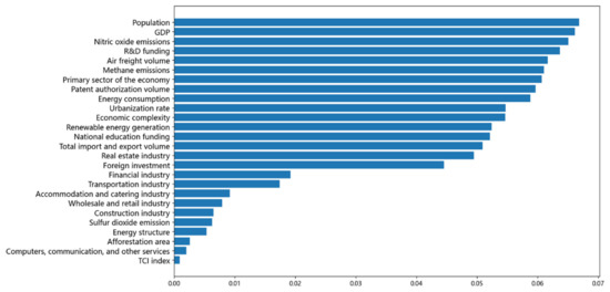
Figure 4.
The importance of 26 influencing factor characteristics.
According to Figure 4, the importance of influencing factors over 0.04 is selected to predict carbon dioxide emissions; these are population, GDP, nitric oxide emissions, research and development (R&D) funding, air freight volume, methane emissions, proportion of primary industry, patent authorization volume, energy consumption, urbanization rate, economic complexity, renewable energy generation, national education funding, total import and export volumes, proportion of real estate industry, and foreign investment. Among these, population and GDP have the greatest impact on carbon dioxide emissions. The larger the population size, the greater the energy demand, and the more carbon dioxide emissions are generated. Coupled with the dependence of economic growth on energy consumption, the trend of carbon dioxide emissions has been increasing. The screened influencing factors can more accurately predict the trend of carbon dioxide emissions.
- (2)
- Ridge Regression Results
To test the reliability of the results of random forest screening, ridge regression was used to analyze various influencing factors. After the addition of the 26 factors of carbon dioxide emissions to the model, the regression coefficients between patent authorization volume and renewable energy generation were not significant; other significant factors match the results of random forest screening. Therefore, the non-significant factors mentioned above were excluded, and other significant factors are the same as those used in the random forest screening.
By incorporating the selected factors into the model for regression and choosing the appropriate K value, the impact of each factor on carbon dioxide emissions can be identified. The results are shown in Table 4.

Table 4.
Updated ridge regression results.
R2 is 0.994, the adjusted R2 is 0.989, the F-statistic is significant at the 0.01 level, and the overall fitting effect is good. These results indicate that the selected factors have high interpretability for carbon dioxide emissions.
As shown in Table 4, the impact of economic complexity on carbon dioxide emissions is relatively large, and the improvement in policy stability promotes an increase in economic complexity [43]. The division of labor between regions and industries is clear, thus promoting efficient economic development. In the short run, carbon dioxide emissions will increase, but in the long run, carbon dioxide emissions will inevitably be controlled. Because the chosen urbanization level reflects the population urbanization rate, and there is an inverted U-shaped relationship between urbanization and carbon emissions [45], an effective urbanization process can be gradually adopted to suppress the increase in carbon emissions. Energy consumption should be reduced, the stable growth of GDP and population should be controlled, and high-energy-consuming industries should be upgraded. R&D funding has a positive impact on carbon dioxide emissions, which follows a non-linear relationship [46]. An increase in R&D intensity can only reduce carbon dioxide emissions when R&D intensity reaches a certain level. Therefore, it is necessary to increase R&D investment and national education funding and to suppress carbon dioxide emissions through inflection points.
Although the relationship between influencing factors and carbon emissions has been obtained, the fitting effect of the model and its prediction accuracy are insufficient. The results of ridge regression prediction and true values are shown in Figure 5.
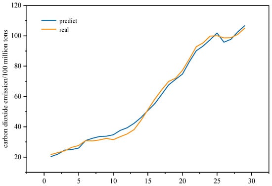
Figure 5.
Ridge regression fitting plot.
Therefore, the ridge regression model is more suitable for analyzing the relationship between influencing factors and carbon dioxide emissions. This paper searches for a better prediction model to predict the dynamic evolution trend of carbon dioxide emissions.
3.3.2. Model Selection
Data from 1990 to 2015 were selected to train the model, and data from 2016 to 2019 were selected as the test set. Then, carbon dioxide emissions data were predicted using the SVR, SSA-SVR, LSTM, and SSA-LSTM models, where SSA-SVR and SSA-LSTM optimize the parameters of the SVR and LSTM models using SSA. The MAE, MSE, MAPE, and R2 of the four models are shown in Table 5.

Table 5.
Performance indicators of the models.
Based on the four evaluation indicators shown in Table 5, the MSE, MAE, and MAPE values of SSA-LSTM are the smallest, and its R2 is the closest to 1, reaching 0.9708. The SSA-LSTM model achieves the best performance on all four evaluation indicators and achieves higher predictive accuracy. Therefore, this paper selects the SSA-LSTM model for prediction. The parameter optimization of the SSA-LSTM model and the model fitting effect from 1990 to 2019 are shown in Figure 6, Figure 7 and Figure 8.
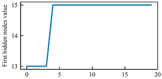
Figure 6.
Hidden layer neuron iteration curve.
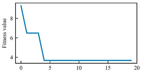
Figure 7.
Fitness iteration curve.
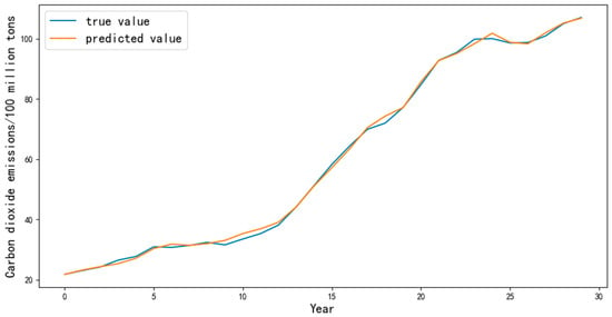
Figure 8.
Fitting results between SSA-LSTM predicted values and true values.
Figure 8 shows that the SSA-LSTM model achieves a good fitting effect in predicting carbon dioxide emissions and can more accurately capture the situation and values of the carbon peak, which meets the research needs of this paper.
3.3.3. Scenario Setting
The meaning of control indicators refers to their ability to control corresponding indicators through macro policy guidance, environmental regulations, and other policy measures. Non-controlling indicators are more influenced by past data and the market, and they will develop according to a certain level of inertia. Therefore, it is advisable to use appropriate models for their prediction. This paper uses the G (1,1) model to predict non-controlling indicators.
The setting of carbon peak scenario prediction parameters requires the consideration of multiple factors. The following presents several parameters that can be macro controlled by policies.
- (1)
- GDP
The prediction of carbon peak scenarios needs to consider the economic development trend. As China is still a developing country, pursuing moderate economic growth for a considerable period of time is a necessary condition to achieve national prosperity and strength. Therefore, the dual carbon target cannot be achieved by reducing the economic growth rate, making it necessary to set a reasonable annual GDP growth rate. According to the “Research Report on Carbon peak in China before 2030” [47], it has been estimated that China will achieve carbon peak in the 14th Five Year Plan and 15th Five Year Plan period. The average GDP growth rate exceeded 5% every year, and the GDP of 2035 was projected to double compared to the 2020 level; therefore, China’s average annual GDP growth rate was set to 5.5% from 2021 to 2030 and to 4.5% from 2030 to 2040. This setting is used as the benchmark scenario. According to the World and China Energy Outlook 2060 [48], the average annual growth rate of China’s GDP before 2025 is about 4.8%, and from 2025 to 2060, it is 3.1%, which is considered a low-carbon scenario. The average annual growth rate of GDP from 2021 to 2030 was set to 6.89%, and from 2030 to 2040, it was set to 6.31% [49], which is considered an extensive scenario.
- (2)
- Population
The population growth rate also impacts carbon emissions; therefore, it is necessary to consider expected changes in the population growth rate. Chen et al. [50] used the population growth rate from 2020 to 2030 to predict the total population in the future, predicting the total population of China to reach 1412 million in 2025, 1424 million in 2030, and 1440 million in 2040. This is considered the benchmark scenario. The China Petroleum Economic and Technological Research Institute [48] predicted that the population of China will reach a peak of 1.43 billion people by 2030, followed by a slow decline, and a decrease to 1.3 billion people by 2060. In this paper, this is used as the low-carbon scenario. The analysis of designated scenarios was conducted according to the National Population Development Plan [51]. In this paper, the population is set to reach 1448 million in 2025, 1488 million in 2030, 1529 million in 2035, and 1567 million in 2040, which represents an extensive scenario.
- (3)
- Urbanization rate
Because of the inverted U-shaped relationship between urbanization and carbon emissions [9], effective urbanization processes can be gradually adopted to suppress the increase in carbon emissions. According to the “fourteen” proposed by Ou et al. [52], China’s urbanization rate will generally follow a stable and slowing trend during the Five Year Plan period. The average annual growth rate from 2020 to 2025 will remain at around 0.71%, and it is expected to reach around 72.2% in 2025, 73.5% in 2035, and 74.9% in 2040 [49]. In this paper, this serves as the benchmark scenario. Under the new pattern of “dual circulation”, the urbanization rate continues to increase fueled by new urbanization policies. It is expected that the urbanization rate will reach around 70% in 2030 and further increase to around 80% in 2060, which is considered a low-carbon scenario. According to the benchmark scenario and current data statistics, the urbanization rate in 2020 was 63.9%, the average annual growth rate of urbanization remained at 1.32% from 2020 to 2025, and the urbanization rate will reach around 74% in 2030, 76.4% in 2035, and 78% in 2040. This serves as the extensive scenario.
- (4)
- Energy consumption
Carbon emissions are closely related to energy consumption; therefore, to substantially control carbon dioxide emissions, it is necessary to control energy consumption. The 14th Five Year Plan requires a decrease of 13.5% in energy consumption per unit of GDP by 2025 and requires energy consumption to be at the same level as that of the 13th Five Year Plan. In the benchmark scenario, this paper sets an annual growth rate of −3.40% for energy intensity from 2020 to 2030 and a rate of −2.7% from 2030 to 2039. The low-carbon scenario is characterized by an average annual growth rate of −3.90% from 2020 to 2030 and a rate of −3.2% from 2030 to 2039. The average annual growth rate of energy intensity is −2.5% from 2020 to 2030 and −2% from 2020 to 2033, which is considered an extensive scenario. Energy consumption can be obtained by setting energy intensity and GDP and by increasing the efforts of low-carbon transformation in the energy industry. Scenario parameter settings are shown in Table 6, Table 7 and Table 8

Table 6.
Benchmark scenario parameter setting.

Table 7.
Low-carbon scenario parameter setting.

Table 8.
Extensive scenario parameter setting.
3.3.4. Prediction Results
In these three scenarios, this paper can obtain the carbon peak time and peak value under the prediction of the SSA-LSTM model. These are shown in Figure 9 and Figure 10.
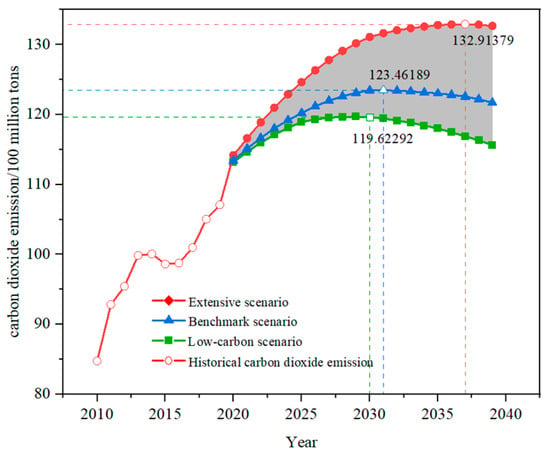
Figure 9.
Peak time for three scenarios.
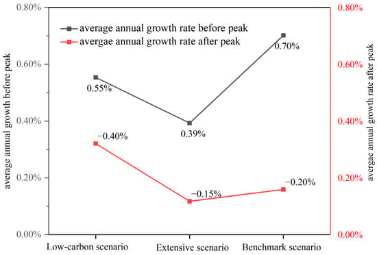
Figure 10.
Average annual growth rate of carbon dioxide emissions.
The carbon peak time of the benchmark scenario is 2031, with a peak of 12.346 billion tons. The carbon peak time of the low-carbon scenario is 2030, with a peak of 11.962 billion tons. In the extensive scenario, the peak time is 2037, with a peak of 13.291 billion tons, which is 945 million tons higher than the peak of the benchmark scenario and 1329 million tons higher than the peak of the low-carbon scenario. The high peak will also have a considerable impact on the environment.
Figure 9 shows that under the three scenarios, the peak value is relatively high and the post peak change rate is small; the decrease in carbon dioxide emissions is relatively stable, and without strict constraints on the economy and energy, it will be challenging for China to achieve carbon neutrality by 2060. Moreover, Figure 10 shows that the change rates before and after the peak value differ between the three scenarios. In the benchmark scenario, the average annual growth rate before the peak is 0.7%, and the average annual growth after the peak is −0.2%. In the low-carbon scenario, the average annual growth rate before the peak is 0.55%, and the average annual growth after the peak is −0.4%. In the extensive scenario, the average annual growth rate before the peak is 0.39%, and the average annual growth after the peak is −0.15%. The increasing rate before reaching the peak is higher than the rate of decrease after reaching the peak. By constraining factors such as the economy, energy consumption, population, and urbanization rate, the degree of carbon dioxide emissions reduction is limited; therefore, the level of technological innovation should be improved and carbon dioxide emissions should be reduced from the perspective of energy use efficiency.
Therefore, we consider the impact of GDP growth, population growth, energy consumption, and technological progress on carbon dioxide emissions, because the energy consumption in this paper is calculated from energy intensity, and energy consumption is linked to technological progress; so based on the baseline scenario, low-carbon scenario, and extensive scenario, this paper sets the scenarios of low economic development, low population growth, and technological progress, except for the GDP (population or energy intensity) in the low-carbon scenario, other factors are set as in the baseline scenario, so as to compare with the baseline scenario. The low-carbon scenario and the extensive scenario were compared to observe the impact of changes in different factors on carbon dioxide emissions. Six scenario settings and results are shown in Table 9 and Table 10.

Table 9.
Six scenarios’ parameter setting.

Table 10.
Peak results in six scenarios.
According to Figure 11, in the low economic development scenario, GDP is set according to the low-carbon scenario, while other parameters are set according to the baseline scenario. The peak and peak times were similar to the baseline scenario and did not change significantly. In the low population growth scenario, the population is set according to the low-carbon scenario, while the other parameters are set according to the baseline scenario. The peak time is in 2030, with a peak of 12.372 billion tons, similar to the baseline scenario, with no significant change in the peak. Under the technological progress scenario, energy intensity is set according to the low-carbon scenario, and other parameters are set according to the baseline scenario, with carbon dioxide emissions peaking at 11.98 billion tons in 2034, similar to the low-carbon scenario. It can be concluded that energy intensity is a key factor in reducing the peak, i.e., technological progress; therefore, the level of technological innovation should be increased from the perspective of energy efficiency to reduce carbon dioxide emissions.
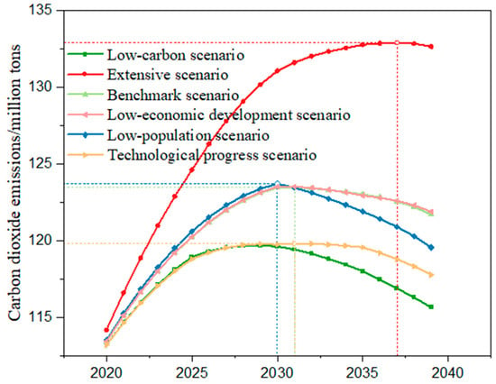
Figure 11.
Peak time for six scenarios.
4. Conclusions
Based on random forest and ridge regression methods, this paper identifies the key influencing factors of China’s carbon dioxide emissions. The SSA-LSTM model with the best prediction effect on China’s carbon dioxide emissions was selected to predict the evolution trend of China’s carbon dioxide emissions under the three scenarios of the benchmark scenario, low-carbon scenario, and extensive scenario. The following conclusions are obtained:
- (1)
- Decoupling analysis shows that China’s GDP and carbon dioxide emissions were generally in a weak decoupling state between 1990 and 2019. In addition, SSA-LSTM achieves a higher accuracy in predicting carbon dioxide emissions, which can better predict the peak level and peak time of carbon dioxide emissions. The SSA-LSTM model can also be used to predict the trends of carbon dioxide emissions in other countries.
- (2)
- The scenario analysis result indicates that under both the low-carbon scenario and benchmark scenario, China can achieve the carbon peak goal at around 2030. Under the extensive scenario, the time when carbon peak will be achieved is postponed to 2037, and the peak is 945 million tons and 1329 million tons higher compared to the peaks of the benchmark scenario and low-carbon scenario, respectively. Therefore, China should develop towards a low-carbon scenario in the future to minimize detrimental impacts on the environment. Through the scenarios of low economic development, low population growth, and technological progress, it can be concluded that energy intensity is the key factor in reducing the peak.
Important policy inspirations of this study are summarized as follows: To achieve the carbon peak target on schedule, China needs to drive the relationship between GDP and carbon dioxide emissions from a weak decoupling state to a strong decoupling state. This means that China needs to break away from the old path represented by both the extensive development scenario and the benchmark development scenario and enter a new path of low-carbon development. While maintaining stable economic growth, China should focus on improving the technological level and reducing energy intensity to move towards a new low-carbon development path. The research presented in this paper has a certain reference value for China to formulate carbon dioxide emissions reduction policies and can also provide theoretical insight for global sustainable development.
Author Contributions
Conceptualization, Z.Y.; Methodology, Z.Y.; Writing—Reviewing and Editing, Z.Y.; Writing Original draft preparation, X.W.; Software, X.W.; Data, X.W.; Supervision, Y.S.; Investigation, Y.S.; Visualization, J.P.; Validation, J.P. All authors have read and agreed to the published version of the manuscript.
Funding
This research was funded by the Major Program of the National Social Science Fund of China, grant number 17ZDA092; and the special project of “College Quality Education and Digital Curriculum Construction” in Jiangsu Province in 2020, grant number 2020JDKT032.
Institutional Review Board Statement
Not applicable.
Informed Consent Statement
Not applicable.
Data Availability Statement
No new data were created or analyzed in this study. Data sharing is not applicable to this article.
Conflicts of Interest
The authors declare no conflicts of interest.
References
- Liu, Z.K.; Jiang, P.; Wang, J.Z.; Zhang, L.F. Ensemble system for short term carbon dioxide emissions forecasting based on multi-objective tangent search algorithm. J. Environ. Manag. 2022, 302, 113951. [Google Scholar] [CrossRef] [PubMed]
- IEA. International Energy Agency. 2021. Available online: https://www.iea.org (accessed on 15 July 2023).
- State Council. Carbon Reduction, China Sets Hard Targets. 2020. Available online: http://www.gov.cn/xinwen/2020-09/30/content_5548478.htm (accessed on 15 May 2023).
- Cai, B.F.; Cao, L.B.; Lei, Y.; Wang, C.; Zhang, L.; Zhu, J.H.; Li, M.Y.; Du, M.B.; Lv, C.; Jiang, H.Y.; et al. Carbon dioxide emissions pathways under China’s carbon neutrality goal. China Popul. Resour. Environ. 2021, 31, 7–11. (In Chinese) [Google Scholar]
- Song, M.L.; Wang, S.H.; Yu, H.Y.; Yang, L.; Wu, J. To reduce energy consumption and to maintain rapid economic growth: Analysis of the condition in China based on expended IPAT model. Renew. Sustain. Energy Rev. 2011, 15, 5129–5134. [Google Scholar] [CrossRef]
- Central People’s Government of the People’s Republic of China. Proposal of the Central Committee of the Communist Party of China on Formulating the 14th Five Year Plan for National Economic and Social Development and the Long-Range Goals for 2035. 2020. Available online: https://www.gov.cn/zhengce/2020-11/03/content_5556991.htm (accessed on 10 August 2023).
- Central People’s Government of the People’s Republic of China. The State Council’s (2021) Action Plan for Carbon Peak before 2030. 2021. Available online: https://www.gov.cn/zhengce/content/2021-10/26/content_5644984.htm (accessed on 26 May 2023).
- He, L.H.; Yang, P.; Meng, Y.L.; Kong, Y. The potential contribution of energy structure optimization to low-carbon Shandong. China Popul. Resour. Environ. 2015, 25, 89–97. (In Chinese) [Google Scholar]
- Wang, Z.Q.; Jia, X.M. Analysis of energy consumption structure on CO2 emission and economic sustainable growth. Energy Rep. 2022, 8, 1667–1679. [Google Scholar] [CrossRef]
- Zhang, C.L.; Zhang, F. The impact of ecological protection and industrial structure upgrading on carbon emission: An empirical study based on data from the Yangtze River Economic Belt. Stat. Decis. 2022, 38, 77–80. (In Chinese) [Google Scholar]
- Gu, Q.K.; Lin, L.F. Effectiveness, influencing factors, and peak path of carbon reduction in the manufacturing industry under the “dual carbon” target: Panel data analysis based on major manufacturing provinces. Econ. Issues 2024, 2, 57–63. [Google Scholar]
- Liu, M.Z.; Yang, X.T.; Wen, J.X.; Wang, H.; Feng, Y.; Lu, J.; Chen, H.; Wu, J.; Wang, J. Drivers of China’s carbon dioxide emissions: Based on the combination model of structural decomposition analysis and input-output subsystem method. Environ. Impact Assess. Rev. 2023, 100, 107043. [Google Scholar] [CrossRef]
- Shahbaz, M.; Raghutla, C.; Song, M.; Zameer, H.; Jiao, Z. Public-private partnerships investment in energy as new determinant of CO2 emissions: The role of technological innovations in China. Energy Econ. 2020, 86, 104664. [Google Scholar] [CrossRef]
- Chen, C.H.; Luo, Y.Q.; Zou, H.; Huang, J.B. Understanding the driving factors and finding the pathway to mitigating carbon emissions in China’s Yangtze River Delta region. Energy 2023, 278, 127897. [Google Scholar] [CrossRef]
- Liu, Z.M.; Liu, X.Z.; Zhu, H.Y.; He, M.H. Evaluation of Carbon Peaking in China’s Provinces from the Perspective of Water Energy Grain System Coupling: Analysis Based on LEAP Model. Econ. Geogr. 2024, 44, 118–129. (In Chinese) [Google Scholar]
- Lin, B.Q.; Liu, X.Y. Carbon emission during China’s urbanization stage: Influencing factors and emission reduction strategies. Econ. Res. 2011, 8, 66–78. (In Chinese) [Google Scholar]
- Li, B.; Zhang, J.B.; Li, H.P. Temporal and spatial characteristics of carbon emission from agriculture in China and decomposition of influencing factors. China Popul. Resour. Environ. 2011, 21, 80–86. (In Chinese) [Google Scholar]
- Liang, W.; Gan, T.; Zhang, W. Dynamic evolution of characteristics and decomposition of factors influencing industrial carbon dioxide emissions in China: 1991–2015. Struct. Chang. Econ. Dyn. 2019, 49, 93–106. [Google Scholar] [CrossRef]
- Shuai, C.Y.; Chen, X.; Wu, Y.; Tan, Y.; Zhang, Y.; Shen, L. Identifying the key impact factors of carbon emission in China: Results from a largely expanded pool of potential impact factors. J. Clean. Prod. 2018, 175, 612–623. [Google Scholar] [CrossRef]
- Chen, Z.M.; Wu, S.M.; Ma, W.B.; Liu, X.M. Analysis of influencing factors on carbon dioxide emissions in cities above prefecture level in China: Based on the extended STIRPAT model. China Popul. Resour. Environ. 2018, 10, 45–54. (In Chinese) [Google Scholar]
- Zhao, Y.; Duan, X.Y.; Yu, M. Calculating carbon emissions and selecting carbon peak scheme for infrastructure construction in Liaoning Province, China. J. Clean. Prod. 2023, 420, 138396. [Google Scholar] [CrossRef]
- Liu, W.D.; Tang, Z.P.; Xia, Y.; Han, M.Y.; Jiang W., B. Machine learning identification and evolution of key influencing factors on carbon intensity in China. Acta Geogr. Sin. 2019, 74, 2592–2603. (In Chinese) [Google Scholar]
- Qin, J.H.; Gong, N.J. The estimation of the carbon dioxide emissions and driving factors in China based on machine learning methods. Sustain. Prod. Consum. 2022, 33, 218–229. [Google Scholar] [CrossRef]
- Wu, Y.; Xu, B. When will China’s carbon emissions peak? Evidence from judgment criteria and emissions reduction paths. Energy Rep. 2022, 8, 8722–8735. [Google Scholar] [CrossRef]
- Li, R.; Liu, Q.Q.; Cai, W.G.; Liu, Y.; Yu, Y.H.; Zhang, Y.H. Echelon peaking path of China’s provincial building carbon emissions: Considering peak and time constraints. Energy 2023, 271, 127003. [Google Scholar] [CrossRef]
- Wang, Y.; Bi, Y.; Wang, A.D. Scenario prediction and emission reduction potential assessment of China’s industrial carbon emission peaking. China Popul. Resour. Environ. 2017, 27, 131–137. (In Chinese) [Google Scholar]
- Liu, D.N.; Xiao, B.W. Can China achieve its carbon emission peaking? A scenario analysis based on STIRPAT and system dynamics model. Ecol. Indic. 2018, 93, 647–657. [Google Scholar] [CrossRef]
- Liu, X.; Wang, X.; Meng, X. Carbon Emission Scenario Prediction and Peak Path Selection in China. Energies 2023, 16, 2276. [Google Scholar] [CrossRef]
- Zeng, Q.S.; Shi, C.F.; Zhu, W.J.; Zhi, J.Q.; Na, X.H. Sequential data-driven carbon peak path simulation research of the Yangtze River Delta urban agglomeration based on semantic mining and heuristic algorithm optimization. Energy 2023, 285, 129415. [Google Scholar] [CrossRef]
- Zhu, C.Z.; Wang, M.; Du, W.B. Prediction on Peak Values of carbon dioxide emissions from the Chinese Transportation Industry Based on the SVR Model and Scenario Analysis. J. Adv. Transp. 2020, 1–14. [Google Scholar] [CrossRef]
- Wei, S.; Wang, Y.W.; Zhang, C.C. Forecasting CO2 emissions in Hebei, China, through moth-flame optimization based on the random forest and extreme learning machine. Environ. Sci. Pollut. Res. 2018, 25, 28985–28997. [Google Scholar] [CrossRef] [PubMed]
- Huo, Z.; Zha, X.; Lu, M.; Ma, T.; Lu, Z. Prediction of Carbon Emission of the Transportation Sector in Jiangsu Province-Regression Prediction Model Based on GA-SVM. Sustainability 2023, 15, 3631. [Google Scholar] [CrossRef]
- Pan, S.Y.; Zhang, M.L. Research on carbon dioxide emissions Prediction and Influencing Factors in Gansu Province Based on BP Neural Network. Environ. Eng. 2023, 41, 61–68. (In Chinese) [Google Scholar]
- Pu, X.; Yao, J.; Zheng, R. Forecast of Energy Consumption and Carbon Emissions in China’s Building Sector to 2060. Energies 2022, 15, 4950. [Google Scholar] [CrossRef]
- Zhao, J.H.; Li, J.S.; Wang, P.L.; Hou, G.J. Research on Carbon Peak Path in Henan Province Based on Lasso BP Neural Network Model. Environ. Eng. 2022, 40, 151–156. (In Chinese) [Google Scholar]
- Li, G.Z.; Huang, Q.H. Prediction of Beijing-Tianjin-Hebei carbon peak scenario based on Lasso-GRNN neural network model. Environ. Sci. 2024, 1–21. (In Chinese) [Google Scholar]
- Shi, C.F.; Zhi, J.Q.; Yao, X.; Zhang, H.; Yu, Y.; Zeng, Q.; Li, L.; Zhang, Y. How can China achieve the 2030 carbon peak goal—A crossover analysis based on low-carbon economics and deep learning. Energy 2023, 269, 2–15. [Google Scholar] [CrossRef]
- Wu, Y.X.; Wu, Q.B.; Zhu, J.Q. Improved EEMD-based crude oil price forecasting using LSTM networks. Stat. Mech. Appl. 2019, 516, 114–124. [Google Scholar] [CrossRef]
- Li, Y.; Huang, S.Y.; Miao, L.; Wu, Z. Simulation analysis of carbon peak path in China from a multi-scenario perspective: Evidence from random forest and back propagation neural network models. Environ. Sci. Pollut. Res. 2023, 30, 46711–46726. [Google Scholar] [CrossRef] [PubMed]
- Xue, J.K.; Shen, B. A novel swarm intelligence optimization approach: Sparrow search algorithm. Syst. Sci. Control Eng. 2020, 8, 22–34. [Google Scholar] [CrossRef]
- Zhang, J.L.; Wang, X.F.; Lu, L.; Niu, P.F. Comparative Analysis and Research on Several New Intelligent Optimization Algorithms. Comput. Sci. Explor. 2022, 16, 88–105. (In Chinese) [Google Scholar]
- Tang, Y.; Dai, Q.; Yang, M.Y.; Chen, L.F. Improving Sparrow Search Algorithm to Optimize SVM for Anomaly Detection. Comput. Eng. Sci. 2023, 45, 346–354. (In Chinese) [Google Scholar]
- Wang, X.L.; Qian, D.B.; Shi, H.Y.; Li, M. Science and Technology Innovation, Policy Stability, and Economic Complexity. Financ. Theory Res. 2022, 2, 40–50. (In Chinese) [Google Scholar]
- Lin, Y. Theoretical Basis and Development Direction of New Structural Economics. Econ. Rev. 2017, 3, 4–16. (In Chinese) [Google Scholar]
- Wang, F.; Zhou, X. Population Structure, Urbanization, and Carbon Emission: An Empirical Study Based on Cross border Panel Data. China Popul. Sci. 2012, 2, 47–56. (In Chinese) [Google Scholar]
- Zhang, W.J.; Ren, R.M. The impact of R&D and trade investment on China’s industrial carbon dioxide emissions. Manag. Mod. 2014, 34, 67–68. (In Chinese) [Google Scholar]
- Global Energy Internet Development Cooperation Organization. Research Report on China’s Carbon Peak before 2030; Global Energy Internet Development Cooperation Organization: Beijing, China, 2021. [Google Scholar]
- China Institute of Petroleum Economics and Technology. World and China Energy Outlook for 2060; China Institute of Petroleum Economics and Technology: Beijing, China, 2021. [Google Scholar]
- Bi, C. Research on the Peak Carbon Emission Scheme and Policy of China’s Energy Activities. Sci. Technol. Innov. Rep. 2015, 5, 16–19. (In Chinese) [Google Scholar]
- Chen, X.; Xiao, L. Improvement of Logistic Model and Population Prediction in China. J. Chengdu Univ. Inf. Technol. 2020, 35, 239–243. (In Chinese) [Google Scholar]
- Central People’s Government of the People’s Republic of China. National Population Development Plan (2016–2030). 2016. Available online: https://www.gov.cn/zhengce/content/2017-01/25/content_5163309.htm (accessed on 15 May 2023).
- Ou, Y.H.; Li, Z.; Li, P.L. The Changing Trends and Policy Implications of China’s Urbanization Rate during the 14th Five Year Plan Period. Urban Dev. Res. 2021, 28, 1–9. (In Chinese) [Google Scholar]
Disclaimer/Publisher’s Note: The statements, opinions and data contained in all publications are solely those of the individual author(s) and contributor(s) and not of MDPI and/or the editor(s). MDPI and/or the editor(s) disclaim responsibility for any injury to people or property resulting from any ideas, methods, instructions or products referred to in the content. |
© 2024 by the authors. Licensee MDPI, Basel, Switzerland. This article is an open access article distributed under the terms and conditions of the Creative Commons Attribution (CC BY) license (https://creativecommons.org/licenses/by/4.0/).