Improving Air Quality Prediction via Self-Supervision Masked Air Modeling

Abstract

Presently, the harm to human health created by air pollution has greatly drawn public attention, in particular, vehicle emissions including nitrogen oxides as well as particulate matter. How to predict air quality, e.g., pollutant concentration, efficiently and accurately is a core problem in environmental research. Developing a robust air quality predictive model has become an increasingly important task, holding practical significance in the formulation of effective control policies. Recently, deep learning has progressed significantly in air quality prediction. In this paper, we go one step further and present a neat scheme of masked autoencoders, termed as masked air modeling (MAM), for sequence data self-supervised learning, which addresses the challenges posed by missing data. Specifically, the front end of our pipeline integrates a WRF-CAMx numerical model, which can simulate the process of emission, diffusion, transformation, and removal of pollutants based on atmospheric physics and chemical reactions. Then, the predicted results of WRF-CAMx are concatenated into a time series, and fed into an asymmetric Transformer-based encoder–decoder architecture for pre-training via random masking. Finally, we fine-tune an additional regression network, based on the pre-trained encoder, to predict ozone (O${ }_3$) concentration. Coupling these two designs enables us to consider the atmospheric physics and chemical reactions of pollutants while inheriting the long-range dependency modeling capabilities of the Transformer. The experimental results indicated that our approach effectively enhances the WRF-CAMx model’s predictive capabilities and outperforms pure supervised network solutions. Overall, using advanced self-supervision approaches, our work provides a novel perspective for further improving air quality forecasting, which allows us to increase the smartness and resilience of the air prediction systems. This is due to the fact that accurate prediction of air pollutant concentrations is essential for detecting pollution events and implementing effective response strategies, thereby promoting environmentally sustainable development.

1. Introduction

Air pollution is one of the main environmental issues that has a severe effect on public health [1,2,3]. Urbanization, industrialization and fossil fuel consumption are the main causes of severe air pollution issues. In particular, transportation is a significant contributor to fossil fuel consumption and is associated with devastating health impacts, such as respiratory and cardiovascular diseases, and even death [4,5,6]. During the past few decades, air quality forecasting has become a research hotspot in controlling air pollution. Air pollutant concentration information is crucial for preventing human health issues and strengthening environmental management. Therefore, researchers employ various strategies to predict air pollutant concentrations. These methods can be grouped into two categories [7,8]: (i) deterministic methods based on hypothesis theory and prior knowledge and (ii) statistical methods based on capturing characteristics from data (see Figure 1, left-hand side).

Figure 1. Left: Traditional air prediction pipeline. Right: The proposed masked air modeling framework for improving air quality prediction.

Predicting air pollutant concentrations (APCs) is influenced by various complicated factors. The generation of air pollutants involves intricate chemical reactions in the atmosphere. Furthermore, meteorological factors (e.g., wind speed, temperature, relative humidity, wind direction) influence not only the diffusion of air pollutants, but also photochemical reactions and subsequent concentration changes. Temperature affects atmospheric and ventilation conditions; relative humidity and precipitation alter the deposition characteristics of particulate matter; and wind speed facilitates the diffusion and spread of pollutants [9]. Overall, meteorological forecast deviation, complex chemical processes, uncertainties in pollutant emission inventories, and imperfect parameterization of physical processes in the model lead to errors between the predicted results and measured values [10,11]. Developing a robust model for predicting APCs remains challenging due to inaccurate or missing observations.

To address the above issues, a promising direction lies in data-driven air quality forecast with Artificial Intelligence (AI) models, in particular, deep learning such as Transformer. Transformer [12] is a deep learning model primarily applied in natural language processing tasks. It relies on self-attention mechanisms to process sequential data, enabling it to capture dependencies regardless of their distance in the input sequence. The data-driven simulation optimization can automatically identify patterns and regularities in data. However, this requires a large amount of labeled data. Recently, self-supervised learning via masked autoencoding has been proven to be a promising scheme for learning generalized pre-trained representations [13,14]. For example, BERT [13] uses masked language modeling, achieving state-of-the-art results in tasks like text classification and question-answering. Nevertheless, self-supervised pre-training has not been fully explored in APCs. In fact, due to limited or missing observations, masked autoencoding that removes a portion of the air quality data and learns to predict the removed content is natural and applicable in air quality prediction. We propose a composite model that integrates WRF-CAMx model and a neat scheme of masked autoencoders to accurately predict air pollutant O${ }_3$ concentrations (see Figure 1, right-hand side), which is one of the highest risk factors for global premature mortality [15,16,17]. The main contributions of this research are as follows:

1.

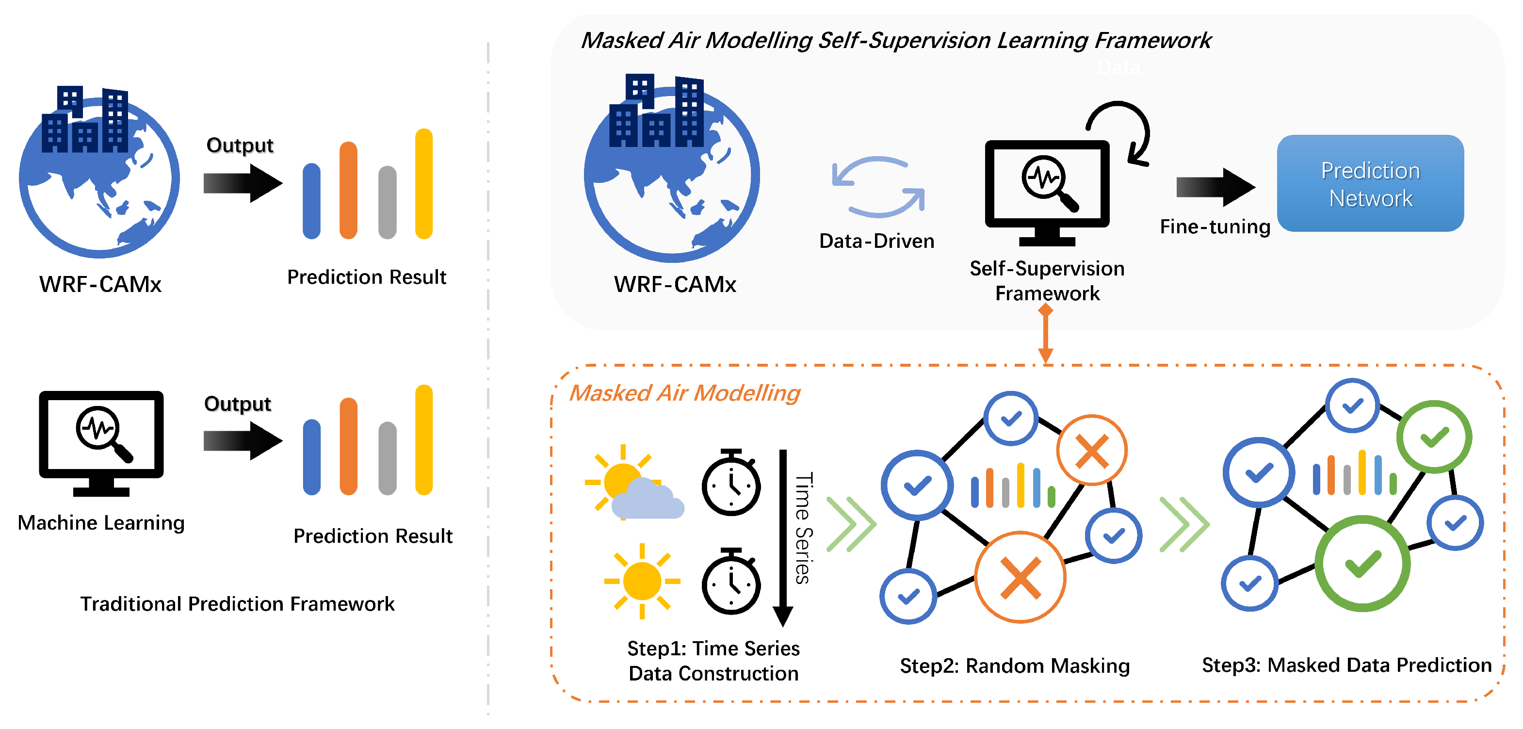
We propose a hybrid air quality prediction pipeline that not only simulates atmospheric physics and chemical reactions of pollutants, but also inherits the long-range dependency modeling capabilities of the Transformer.

2.

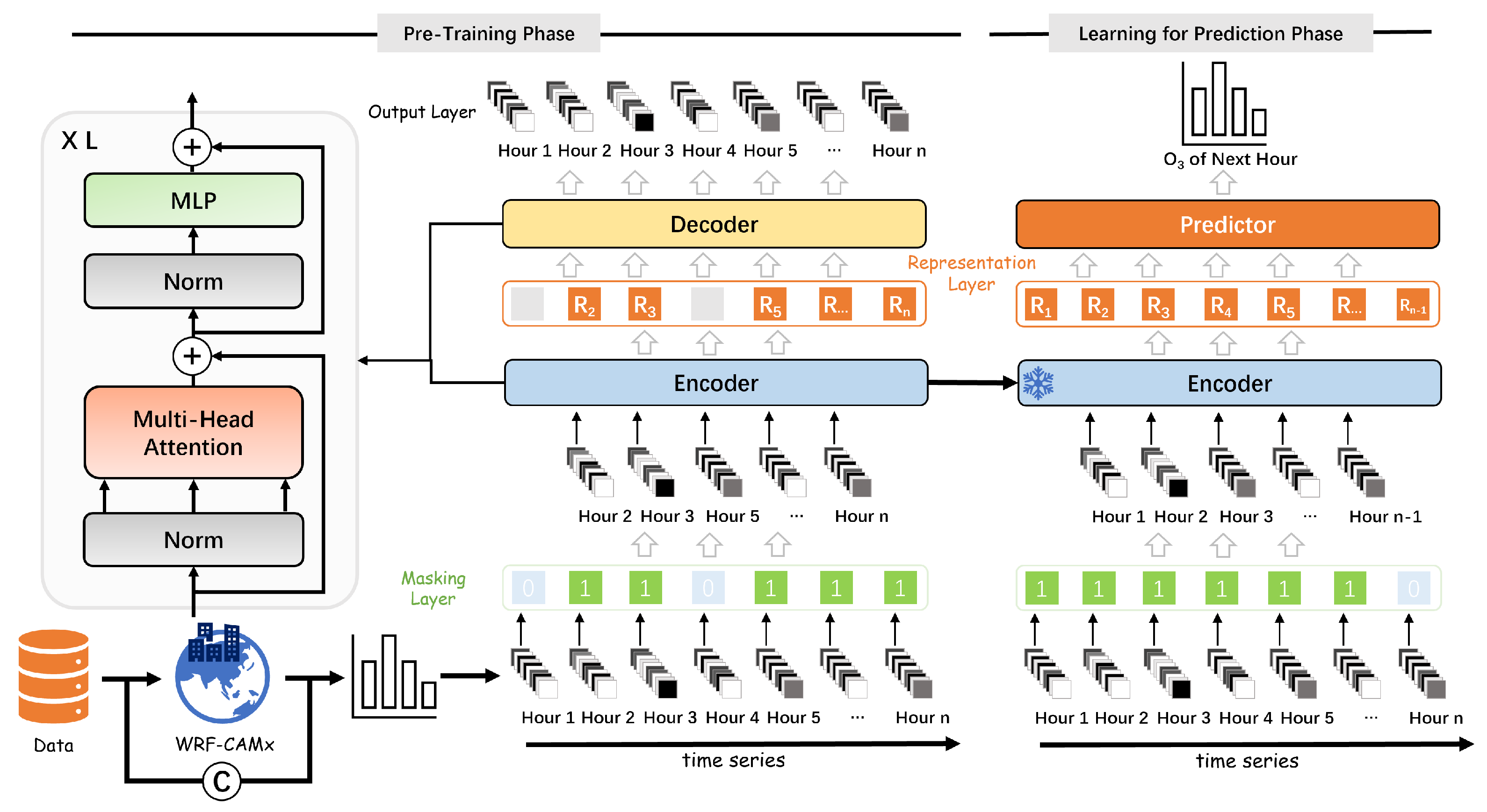
We design an asymmetric Transformer-based encoder–decoder architecture as a promising scheme of masked air modeling, which yields a nontrivial and meaningful self-supervisory sequence representation learning task.

3.

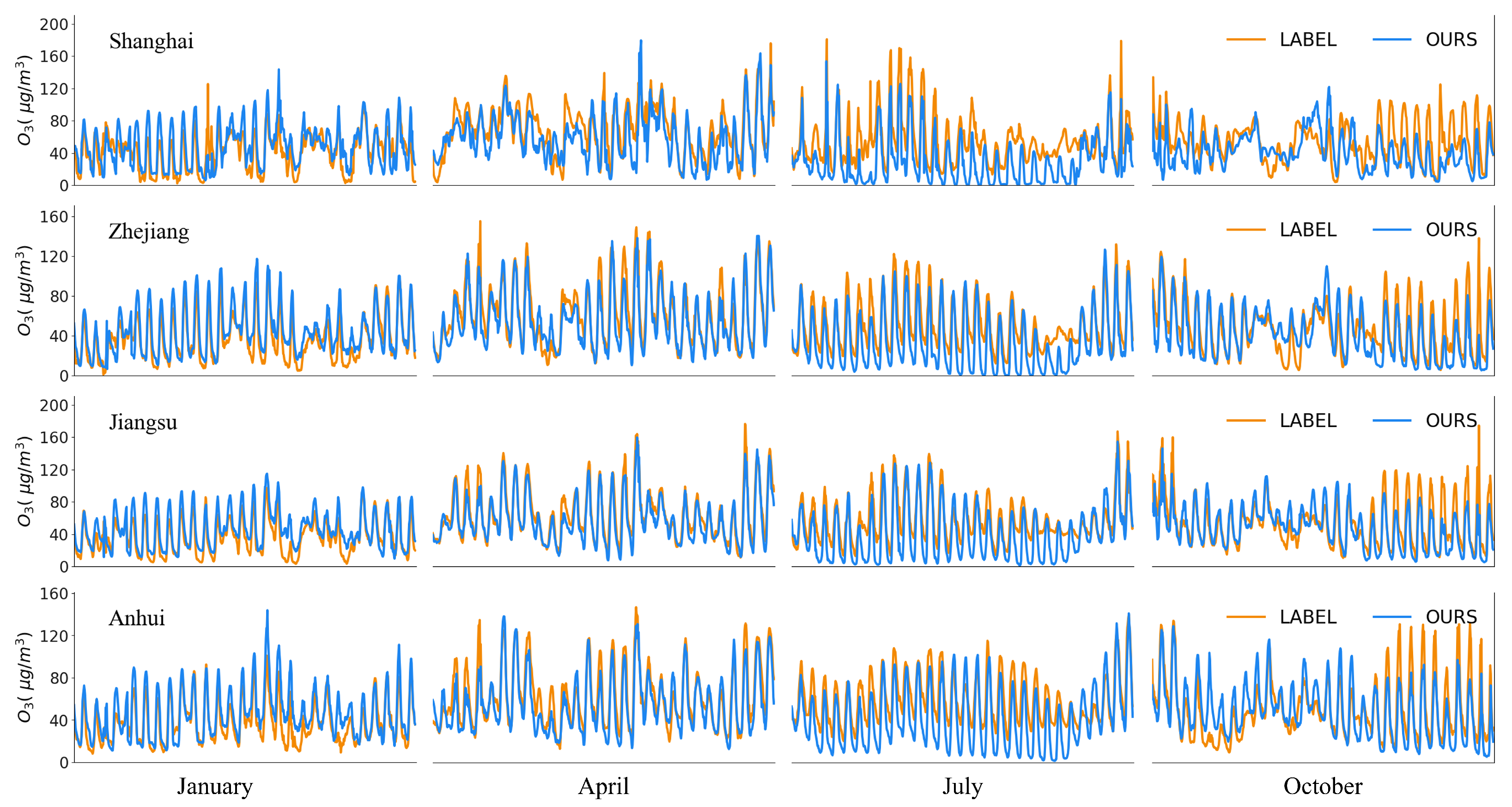
In terms of hour-by-hour simulation performance, the proposed MAM can effectively boost the WRF-CAMx and purely supervisory learning models’ predictive capabilities, which provides more than 26 percent (correlation coefficient) of performance improvements.

2. Related Work

According to the features of existing research, air quality forecasting strategies can be grouped into two major categories: deterministic methods and statistical methods.

The structure of a deterministic model is predefined according to certain theoretical assumptions and prior knowledge. Thus, deterministic methods utilize a set of equations describing the atmospheric physical and chemical processes to simulate diffusion with meteorological and other data inputs [7]. Various representative air quality models have been proposed to simulate the complex changes in atmospheric pollutants. The Community Multiscale Air Quality (CMAQ) model [18,19,20], Weather Research and Forecasting model coupled with the Chemistry (WRF–Chem) model [21,22], the Chemical Lagrangian Model of the Stratosphere (CLaMS) [23], and the Comprehensive Air Quality Model with Extensions (CAMx) [24,25] are typically employed in air pollutant concentration forecasting and are widely used in scenario and policy analyses. Although the theoretical understanding of pollutant diffusion mechanisms continues to be enriched and refined, deterministic models are typically associated with sophisticated a priori knowledge, such as determining a model structure using theoretical assumptions and estimating parameters empirically, where the predictive performance is limited [26,27,28]. Furthermore, the accuracy of such methods depends on the abundance of information and data about emission sources. In general, these errors usually fall into two major types: (i) the inherent biases from parameterizing physical processes and discretizing differential equations reduce simulation accuracy and (ii) the internal variability driven by the sensitivity to the initial conditions, such as meteorological fields and emissions.

Unlike deterministic models, statistical methods can avoid using complex theoretical models, gradually emerging in air pollution prediction [29]. Statistical methods aim to capture patterns and regularities between input data and predictive variables, without relying on explicit knowledge of the underlying physical and chemical processes in the atmosphere [7,30]. Statistical methods are typically divided into classical statistical methods and machine learning methods. Classic statistical methods establish a certain statistical relationship (e.g., AutoRegression Integrated Moving Average [31], or Geographically Weighted Regression [32]) by analyzing the forecast and monitoring data within the same time period. Traditional machine learning methods include Support Vector Machine (SVM) [33,34], multilabel classifier based on Bayesian [35], Random Forest [36], hidden Markov model [37], Boosted Regression Trees [38], and XGBoost [39]. In summary, statistical forecasting methods analyze the statistical regularity of pollutants and then predict the pollution trend. However, statistical models tend to severely degrade when simulating extreme episodes. This is due to the fact that the training data are limited in the representation of complex meteorological phenomena and nonlinear patterns [40].

As an emerging research branch of statistical methods, deep learning is able to effectively capture potential nonlinear relationships from data, and its nonlinear relationship’s forecast ability is superior to that of traditional statistical methods. Typical deep learning networks for forecasting air pollution concentrations include Multilayer Perceptron (MLP) [41], Recurrent Neural Network (RNN) [42], Generative Adversarial Network (GAN) [43], Long Short-Term Memory (LSTM) neural network [44], CNN-LSTM model [45], LSTM variants [46], etc. Deep learning methods show satisfactory performance in extracting latent pattern and inherent features from data [47]. Since emission, diffusion, conversion, and removal of air pollutants are dynamic processes that evolve over time, air pollutant prediction is transformed into a time series data forecasting task, and is used to capture the spatiotemporal feature of pollutants.

3. Method

The proposed algorithm consists of two parts: (1) The Weather Research and Forecasting–Comprehensive Air Quality Model with Extensions (WRF-CAMx) model, and (2) a neat scheme of masked autoencoders that reduces uncertainty and improves simulation accuracy. The implementation details are shown in Figure 2.

Figure 2. Schematic illustration of the Transformer-based masked air modeling.

3.1. WRF-CAMx Modeling

The Weather Research and Forecasting (WRF) model provides hourly weather simulation data for subsequent missions. The Comprehensive Air Quality Model with Extensions (CAMx) model is applied to simulate pollutant concentrations, and the WRF output is processed together with the emission inventory as its input. The time resolution of the model forecast results is 1 h.

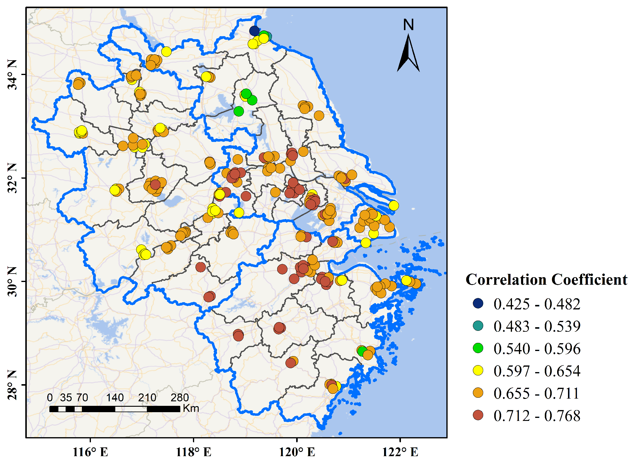
3.1.1. Simulation Domain

The Yangtze River Delta (YRD) region, one of China’s most industrialized regions, is located on the eastern coast of China. The YRD region is composed of 41 cities in the Shanghai municipality, Zhejiang, Jiangsu and Anhui provinces. The air quality issue in the YRD region has consistently attracted considerable attention. For these factors, the YRD region is selected as the research area. The meteorological fields of three successive nested domains with horizontal resolutions of 27 km (d01), 9 km (d02), and 3 km (d03) were simulated by WRF model version 3.9 [25]. The outer domain covers the Chinese mainland, the middle domain covers the eastern part of China, and the inner domain covers the YRD region. CAMx employs a two-layer nested grid with resolution and grid center points identical to the second and third layers of WRF. Each layer of the CAMx grid has slightly smaller coverage than the WRF grid to reduce the influence of boundary fields on simulation results [48,49,50].

3.1.2. Model Building

The Global Final Analysis data provided by the National Centers for Environmental Prediction (NCEP) provides the initial and boundary conditions for the WRF model, with a spatial resolution of 1${ }^{\circ }\times 1^{\circ }$ and a time interval of 6 h. Meteorological data output from the WRF model and emission inventory were inputted into the CAMx version 6.5 model to simulate air pollutant concentrations. The emission inventory of the YRD region provided by the Shanghai Academy of Environmental Sciences was adopted within the inner domain, with a resolution of 4 km. The Multi-resolution Emission Inventory for China (MEIC) developed by Tsinghua University was adopted within the other two domains, with a spatial resolution of 0.25° × 0.25° (http://meicmodel.org.cn) [51,52]. According to the principle of conservation of total emissions, bilinear interpolation was used to interpolate the involved emission inventories to a resolution that matches each nested layer of the CAMx model. The essential parameterization schemes of the WRF-CAMx model are listed in Table 1 [48].

Table 1. The parameterization schemes of the WRF-CAMx model.

Physical parameterization scheme
Longwave radiation	RRTM scheme
Shortwave radiation	Goddard scheme
Land surface	Noah land surface model
Cumulus parameterization	Kain–Fritsch scheme
Planetary boundary layer	YSU scheme
Chemical parameterization scheme
Gas-phase chemical mechanism	CB05
Particulate matter chemistry	SOAP/CF
Dry deposition	Wesely model
Wet deposition	Seinfeld and Pandis model

3.2. Masked Air Modeling

3.2.1. Problem Statement

Given the WRF-CAMx simulation results $\{D_0,D_1,\cdots ,D_{h-1}\}$ of meteorology and air quality for the past (h) time periods, we aimed to predict the real air quality concentration for the next time period ($O_h$). In other words, our goal is to find a mapping for predicting $O_h$, which can be written as

$$f_{\theta }\left(D_0,D_1,\cdots ,D_{h-1}\right)=O_h^{\ast },$$

(1)

where $O_h^{\ast }$ denotes the predicted value for the next time period of the input sequence, and $\theta$ indicates learnable parameters. To infer $\theta$, a popular practice is to directly optimize the error between $O_h$ and $O_h^{\ast }$. However, limited data annotation may result in poor generalization of the model. Therefore, in this work, we focus on leveraging the self-supervised model to learn good sequence representation, then fine-tune downstream tasks, i.e., the prediction of air pollutant O${ }_3$ concentration.

Note that O${ }_3$ concentration is confirmed to exhibit a causal relationship with the air pollution data, e.g., SO${ }_2$, NO${ }_2$, PM${ }_{2.5}$, and meteorological data. Specifically, wind direction determines the direction of dispersion; higher wind speeds accelerate dispersion; and relative humidity and temperatures typically affect the rate of atmospheric chemical reactions. Therefore, four meteorological parameters (temperature, relative humidity, wind direction, and wind speed) and four air pollutant concentrations simulated by CAMx (SO${ }_2$, NO${ }_2$, PM${ }_{2.5}$, and O${ }_3$) are selected as the model input in the research, and we set the time span of the sequence to 12 h. We will detail our masked air modeling in the rest of the section.

3.2.2. Masked Autoencoders for Context Understanding

Masked language and image modeling, which aims to hold out a portion of the input and train networks to predict the masked content, have made great progress on natural language processing (NLP) and computer vision (CV) communities. The preponderance of evidence continues to indicate that this self-supervised learning can produce generalized pre-trained representations for various downstream tasks.

Significant interest in this pre-training paradigm arose following the success of some milestones, e.g., BERT [13] and MAE [14]. However, self-supervised pre-training has not been fully explored in air quality forecasting (AQF). In fact, due to inaccurate or missing observations, the scheme that removes a portion of the air quality data and learns to predict the removed content is natural and applicable in air quality prediction. In this work, we attempt to explore the potential of this pre-training strategy in AQF, and refer to this as masked air modeling (MAM). This practice does not only directly solve the problem of missing data, but also promises to provide excellent representation for prediction tasks through fine-tuning.

Formally, the proposed MAM is a framework of neutral learning paradigm. In this work, following MAE, we leverage a simple Transformer-based autoencoder as an instance to reconstruct the missing signal, given its partial observation. To this end, we randomly select time-continuous samples $[x_1,x_2,\cdots ,x_n]$ (where $x_i=\left[D_i\right]\in {\mathbb{R}}^8$) from the dataset to serve as our sequence input, and mask (i.e., remove) a subset of sequence without replacement based on a uniform distribution. Our training strategy is straightforward. One reason it is straightforward is that the input to the MAM encoder is only on visible unmasked vectors, where the MAM encoder is a ViT [53], including alternating layers of multi-headed self-attention (MSA) and MLP blocks:

$$\begin{array}{c}{P}_0=[x_g;x_1\mathbf{E};x_2\mathbf{E};x_3\mathbf{E};\cdots ;x_m\mathbf{E}]+{\mathbf{E}}_{pos},\end{array}$$

(2)

$$\begin{array}{c}{P}_i^{\ast }=\mathrm{MSA}\left({\mathbf{F}}_N\left(P_{i-1}\right)\right)+P_{i-1},\end{array}$$

(3)

$$\begin{array}{c}{P}_i=\mathrm{MLP}\left({\mathbf{F}}_N\left(P_i^{\ast }\right)\right)+P_i^{\ast },\end{array}$$

(4)

$$\begin{array}{c}i=1,\cdots ,L-1,L\end{array}$$

(5)

where $x_g$ is the learnable global token; ${\mathbf{F}}_N\left(·\right)$ is the normalization layer, which is applied before network blocks (L is the number of blocks); $\mathbf{E}\in {\mathbb{R}}^{K\times D}$ and ${\mathbf{E}}_{pos}$ denote trainable linear projection parameters and position embeddings, respectively. Another reason it is straightforward is that decoder input is the full set of tokens, including (i) encoded visible features and (ii) mask tokens, i.e.,

$$Q=\left[[p_L^g\left|\right|p_L^1];[p_L^g\left|\right|{\mathbf{X}}^1];\cdots ;[p_L^g\left|\right|{\mathbf{X}}^{n-m}]\right]+{\mathbf{D}}_{pos},$$

(6)

where $P_L=[p_L^g;p_L^1;\cdots ;p_L^m]$ is the encoder output, and $\mathcal{X}=[{\mathbf{X}}^1;{\mathbf{X}}^2;\cdots ;{\mathbf{X}}^{n-m}]$ denotes a learnable vector sequence indicating mask tokens, and $\left[·\right|\left|·\right]$ is the concatenation operation. Finally, Q will be fed into another series of Transformer blocks to predict the missing data. The decoder is only used during pre-training to address the missing data problem. Therefore, the architecture of the decoder can be flexibly designed. It is important to notice that unlike the original ViT model, we attach the extra learnable embedding $p_L^g$ to sequence representations, thus enhancing the interaction of local and global features. In the original ViT, $p_L^g$ often acted as a class embedding for the final classification tasks.

3.2.3. Learning Prediction Representation

In order to fulfill air quality prediction, we remove the pre-trained MAM decoder and introduce a predictor, which is applied to the sequence features extracted from the pre-trained MAM encoder. The predictor also consists of alternating layers of MSA and MLP blocks, but here, the extra learnable embedding serves as a “regression token” $\mathrm{𝒵}$, i.e., prediction representation, which is fed into a regression head implemented by an MLP with one hidden layer. During the training phase, the parameters of the encoder are frozen, and only the predictor is trainable, which allows us to facilitate a direct inheritance of the encoder’s powerful context modeling capabilities acquired during the pre-training. In addition, the pre-trained encoder–decoder provides a data augmentation method: the practice involves performing random masking on input sequences, wherein the masks are different for each iteration and so they generate new training samples.

3.2.4. Loss Function

Our approach consists of two targets, namely reconstruction and prediction; both belong to regression tasks. Therefore, in this work, we use simple element-wise mean-squared error (MSE) loss to optimize our model, and we find that this works well in our experiments.

$$\begin{array}{c}{\mathcal{L}}_{recon}=\left|\right|{\mathbf{F}}_D\left({\mathbf{F}}_E\left(\mathbf{x}\right)\right)-\mathbf{x}|{|}_2^2,\end{array}$$

(7)

$$\begin{array}{c}{\mathcal{L}}_{pred}=\left|\right|{\mathbf{F}}_P\left({\mathbf{F}}_E\left(\mathbf{x}\right)\right)-y{\left|\right|}_2^2,\end{array}$$

(8)

where $\mathbf{x}=[x_1,x_2,\cdots ,x_n]$ denotes input sequence; y indicates ground truth label; and ${\mathbf{F}}_E$, ${\mathbf{F}}_D$, and ${\mathbf{F}}_P$ are the encoder, decoder, and predictor, respectively. More complex loss functions are worth exploring, but we will leave that to future works.

4. Experiment

4.1. Ground-Level Air Pollutant Measurements

The Yangtze River Delta region includes a total of 41 cities, as shown in Figure 3. Hourly air pollutant concentration observation data are obtained from National Urban Air Quality Realtime Release Platform (http://www.cnemc.cn/, (accessed on 1 May 2024)). The simulated data of the WRF-CAMx model were extracted according to the longitude and latitude of the air quality monitoring sites and were established in correspondence with the observed data. Air pollution concentration observation data were used as labels for the forecast data, aiming to calculate simulation errors. The experiment involved pollutant concentration and meteorological data from the YRD in January, April, July, and October 2021.

Figure 3. Left: The location of the YRD. Right: The spatial distribution of air quality monitoring sites.

4.2. Performance Metrics

In this section, we focus on the performance of MAM in predicting air pollutant concentrations and compare it against other algorithms. Mean Bias (BIAS), Root-Mean-Squared Error (RSME), Index of Agreement (IOA), and Correlation Coefficient (COR) are applied to evaluate the accuracy of air pollutant concentration predictions. The evaluation metrics are described as follows:

$$BIAS={\displaystyle \frac{1}{N}}\sum _{i=1}^N(x_i-{\widehat{x}}_i)$$

(9)

$$RMSE=\sqrt{{\displaystyle \frac{1}{N}}\sum _{i=1}^N{(x_i-{\widehat{x}}_i)}^2}$$

(10)

$$IOA=1-{\displaystyle \frac{{\sum }_{i=1}^N{(x_i-{\widehat{x}}_i)}^2}{{\sum }_{i=1}^N\left(\right|x_i-\overline{\widehat{x}}|+|{\widehat{x}}_i-\overline{\widehat{x}}{\left|\right)}^2}}$$

(11)

$$COR={\displaystyle \frac{{\sum }_{i=1}^N(x_i-\overline{x})(\widehat{x}-\overline{\widehat{x}})}{\sqrt{{\sum }_{i=1}^N{(x_i-\overline{x})}^2{(\widehat{x}-\overline{\widehat{x}})}^2}}}$$

(12)

where N is the total number of predicted (or monitored) data. $x_i$ represents the simulated value of pollutant concentration. ${\widehat{x}}_i$ represents the monitoring value of air pollutant concentration. $\overline{x}$ is the mean of $\left\{x_1,...,x_N\right\}$ and $\overline{\widehat{x}}$ is defined in the same way.

4.3. Results and Discussion

To verify the effectiveness of MAM, we designed a series of experiments on the obtained air quality dataset, including simulated data and corresponding monitoring data in the Yangtze River Delta. A 10-fold cross-validation method was applied to assess the performance or effectiveness of various methods. The input dataset was split into ten equally sized subsets called folds. The model was trained and tested ten times. During each evaluation process, nine folds were used as the training set and the remaining one fold was used for validation. This evaluation process was repeated ten times to ensure that each fold was tested. For each assessment of the proposed model performance, BIAS ($\mathrm{\mu }\mathrm{g}/{\mathrm{m}}^3$), RSME ($\mathrm{\mu }\mathrm{g}/{\mathrm{m}}^3$), IOA, and COR were employed as statistical indicators to quantify the accuracy of O${ }_3$ simulations.

4.3.1. Comparison with Baseline

To test the performance of our self-supervised framework, we compared our method with the baseline (WRF-CAMx model). Cross-validation results on the air quality dataset (i.e., O${ }_3$) are shown in Figure 4. Overall, the proposed MAM performed better than the baseline, with higher IOA and COR, and lower BIAS and RMSE. O${ }_3$ concentrations varied in different seasons. January, April, July, and October were selected to represent winter, spring, summer, and autumn, respectively. According to the Mean Bias shown in Figure 4, the hourly O${ }_3$ concentration data simulated by WRF-CAMx in the YRD region are generally lower than the monitoring station data. This phenomenon is more obvious in April.

Figure 4. Scatter density plots of cross-validation results for the WRF-CAMx model (left) and our MAM model (right). Cells with aggregate counts up to 1% of the total will be colored. Each row from top to bottom represents the simulation results in January, April, July, and October, respectively.

Our MAM framework outperformed the WRF-CAMx model in the four months, with a 0.10–0.26 IOA enhancement and a 0.13–0.27 COR increase, demonstrating that MAM has a stable positive effectiveness. To be specific, compared with the WRF-CAMx model, the RMSE of the April simulation results decreased from 40.69 to 22.87, and the IOA increased from 0.60 to 0.86, which is the most obvious change. This may be due to a low accuracy of the WRF-CAMx model; thus, the effect of MAM is obvious. As shown in Figure 4, in April, there is a significant discrepancy between the simulation results of the WRF-CAMx model and the observed data at monitoring stations. Limited knowledge of pollutant sources and imperfect representation of physicochemical processes would pose biases in the predicted results of the WRF-CAMx.

The hour-by-hour time series comparison results of O${ }_3$ concentration in the YRD region (Shanghai, Zhejiang, Jiangsu, and Anhui) are shown in Figure 5. The O${ }_3$ simulated data in the YRD region are divided into four datasets based on administrative areas, and hourly average values are validated against monitoring data. The temporal variation trend and numerical range of the simulated concentration produced by the proposed model are generally consistent with the observed values. Table 2 shows the forecast performance of the proposed method in the four regions, evaluated using correlation coefficients. For the four regions, the simulated hourly O${ }_3$ concentrations in each month are compared with the monitoring data.

Figure 5. Time series comparison. From top to bottom: Shanghai, Zhejiang, Jiangsu, and Anhui. From left to right: January, April, July, and October.

Table 2. Comparison of ozone prediction results. The values represent the average correlation coefficients, and the best are highlighted in bold.

Area	Model	January	April	July	October
Shanghai	Ours WRF-CAMx	0.713 0.411	0.740 0.561	0.696 0.409	0.541 0.456
Zhejiang	Ours WRF-CAMx	0.765 0.551	0.741 0.491	0.753 0.525	0.646 0.525
Jiangsu	Ours WRF-CAMx	0.756 0.545	0.771 0.568	0.711 0.534	0.660 0.554
Anhu	Ours WRF-CAMx	0.731 0.472	0.735 0.413	0.711 0.440	0.615 0.416

In order to further analyze the effectiveness of MAM in air quality forecasting, we validate the predicted results based on the four months of data provided by each monitoring site, shown in Figure 6. Correlation coefficient is used to evaluate the difference between forecast data and monitoring data, where monitoring data are used as labels. The correlation coefficients are visualized in the corresponding geographical locations, and different colors correspond to different levels of correlation coefficients. It can be concluded that MAM achieved satisfactory accuracy in the YRD region. In detail, most of the correlation coefficients range between 0.655 and 0.711, with the highest reaching 0.768. From the results, the proposed MAM is clearly able to produce satisfactory prediction accuracy for different geographical locations in the Yangtze River Delta region.

Figure 6. Air quality prediction accuracy in different geographic locations.

4.3.2. Comparison with Supervision Models

Many supervised learning models are widely used in predicting air pollutant concentration. Therefore, to evaluate the performance gain brought by the pre-training phase, we compared our method with supervised approaches (such as Transformer (w/o MAM), Fully connected Neural Network (FNN), Random Forest (RF)), and WRF-CAMx and Transformer + MAM (w/o WRF-CAMx). In this experiment, all models are tested on the dataset mentioned above, and the performance of each machine learning model is verified by the 10-fold cross-validation method. A comparison of validation results between our method and other models are shown in Table 3. From the results, we found that MAM pre-training can lead to significant improvements in both IOA and COR metrics. It is worth noting that although the Transformer model is more advanced, it does not exhibit a significant advantage over traditional FCN and RF models. Transformer framework often suffers poor generalization when training on a limited dataset, since Transformer lacks certain inductive biases such as locality.

Table 3. Performance comparison of all models. The best are highlighted in bold.

Model	BIAS	RMSE	IOA	COR
Transformer + MAM (Ours)	−4.349	23.627	0.820	0.689
Transformer	−6.678	25.264	0.719	0.596
FNN	29.688	37.421	0.604	0.585
RF	9.864	22.981	0.733	0.584
WRF-CAMx	−12.578	32.403	0.666	0.473
Transformer + MAM (w/o WRF-CAMx)	−4.971	25.171	0.746	0.611

5. Conclusions

In this paper, a deep learning model, termed as masked air modeling (MAM), is proposed to delve into the effectiveness of self-supervised learning in air quality prediction. Moreover, in order to simulate atmospheric physics and chemical reactions of pollutants, we combine conventional atmospheric models (WRF-CAMx) with data-driven deep learning methods. This design leverages the strengths of both approaches to enhance simulation accuracy and predictive capabilities. The experimental results show that in terms of hour-by-hour simulation performance, MAM can effectively boost the model’s robustness, demonstrating its effectiveness. Accurate prediction of atmospheric pollutant concentrations is crucial for formulating strategies to control air pollution, protecting human health, and environmental management.

Even though the proposed self-supervised masked air modeling (MAM) has an advantage in air quality prediction, it often requires large-scale data and computational resources for effective pre-training [54], which may be a potential limitation. Moreover, our method may suffer performance degradation in unseen contexts due to the domain bias between training data and test data. At the same time, the reliance on reconstruction tasks may not always align with downstream tasks, leading to poor generalization in real-world applications. Transformer models can be extended to larger spatial domains, but there are some challenges. For example, a larger spatial domain increases the number of tokens, resulting in higher computational costs and memory usage; this is due to the fact that a Transformer scales quadratically with the number of tokens [12]. That is, scaling to larger spatial domains typically requires more diverse and extensive training data to capture additional variability and complexity. The above challenges may be addressed by using advanced initialization techniques or lightweight Transformer variants. For future work, exploring air pollutant interactions among different locations could provide insights into spatial dependencies and pollutant dispersion patterns. Implementing multi-source data fusion techniques and advanced spatiotemporal models can further improve predictive capabilities and inform effective pollution control strategies.

References

1. Lu, X.; Wang, J.; Yan, Y.; Zhou, L.; Ma, W. Estimating hourly PM2.5 concentrations using Himawari-8 AOD and a DBSCAN-modified deep learning model over the YRDUA, China. Atmos. Pollut. Res. 2021, 12, 183–192. [Google Scholar] [CrossRef]
2. Chen, W.; Tang, H.; He, L.; Zhang, Y.; Ma, W. Co-effect assessment on regional air quality: A perspective of policies and measures with greenhouse gas reduction potential. Sci. Total. Environ. 2022, 851, 158119. [Google Scholar] [CrossRef] [PubMed]
3. Cohen, A.J.; Brauer, M.; Burnett, R.; Anderson, H.R.; Frostad, J.; Estep, K.; Balakrishnan, K.; Brunekreef, B.; Dandona, L.; Dandona, R.; et al. Estimates and 25-year trends of the global burden of disease attributable to ambient air pollution: An analysis of data from the Global Burden of Diseases Study 2015. Lancet 2017, 389, 1907–1918. [Google Scholar] [CrossRef] [PubMed]
4. Zhang, K.; Batterman, S. Air pollution and health risks due to vehicle traffic. Sci. Total. Environ. 2013, 450, 307–316. [Google Scholar] [CrossRef] [PubMed]
5. Mak, H.W.L.; Ng, D.C.Y. Spatial and socio-classification of traffic pollutant emissions and associated mortality rates in high-density hong kong via improved data analytic approaches. Int. J. Environ. Res. Public Health 2021, 18, 6532. [Google Scholar] [CrossRef]
6. Choma, E.F.; Evans, J.S.; Gómez-Ibáñez, J.A.; Di, Q.; Schwartz, J.D.; Hammitt, J.K.; Spengler, J.D. Health benefits of decreases in on-road transportation emissions in the United States from 2008 to 2017. Proc. Natl. Acad. Sci. USA 2021, 118, e2107402118. [Google Scholar] [CrossRef] [PubMed]
7. Yao, J.; Brauer, M.; Raffuse, S.; Henderson, S.B. Machine learning approach to estimate hourly exposure to fine particulate matter for urban, rural, and remote populations during wildfire seasons. Environ. Sci. Technol. 2018, 52, 13239–13249. [Google Scholar] [CrossRef] [PubMed]
8. Li, X.; Peng, L.; Yao, X.; Cui, S.; Hu, Y.; You, C.; Chi, T. Long short-term memory neural network for air pollutant concentration predictions: Method development and evaluation. Environ. Pollut. 2017, 231, 997–1004. [Google Scholar] [CrossRef] [PubMed]
9. Zhang, B.; Rong, Y.; Yong, R.; Qin, D.; Li, M.; Zou, G.; Pan, J. Deep learning for air pollutant concentration prediction: A review. Atmos. Environ. 2022, 290, 119347. [Google Scholar] [CrossRef]
10. Wang, W.; An, X.; Li, Q.; Geng, Y.a.; Yu, H.; Zhou, X. Optimization research on air quality numerical model forecasting effects based on deep learning methods. Atmos. Res. 2022, 271, 106082. [Google Scholar] [CrossRef]
11. Li, H.; Wang, J.; Yang, H.; Wang, Y. Air quality deterministic and probabilistic forecasting system based on hesitant fuzzy sets and nonlinear robust outlier correction. Knowl.-Based Syst. 2022, 237, 107789. [Google Scholar] [CrossRef]
12. Vaswani, A.; Shazeer, N.; Parmar, N.; Uszkoreit, J.; Jones, L.; Gomez, A.N.; Kaiser, Ł.; Polosukhin, I. Attention is all you need. Adv. Neural Inf. Process. Syst. 2017, 30. [Google Scholar]
13. Devlin, J.; Chang, M.W.; Lee, K.; Toutanova, K. Bert: Pre-training of deep bidirectional transformers for language understanding. arXiv, 2018; arXiv:1810.04805. [Google Scholar]
14. He, K.; Chen, X.; Xie, S.; Li, Y.; Dollár, P.; Girshick, R. Masked autoencoders are scalable vision learners. In Proceedings of the IEEE/CVF Conference on Computer Vision and Pattern Recognition, New Orleans, LA, USA, 18–24 June 2022; pp. 16000–16009. [Google Scholar]
15. Zhang, J.; Wei, Y.; Fang, Z. Ozone pollution: A major health hazard worldwide. Front. Immunol. 2019, 10, 2518. [Google Scholar] [CrossRef] [PubMed]
16. Anenberg, S.C.; Horowitz, L.W.; Tong, D.Q.; West, J.J. An estimate of the global burden of anthropogenic ozone and fine particulate matter on premature human mortality using atmospheric modeling. Environ. Health Perspect. 2010, 118, 1189–1195. [Google Scholar] [CrossRef] [PubMed]
17. Turner, M.C.; Jerrett, M.; Pope III, C.A.; Krewski, D.; Gapstur, S.M.; Diver, W.R.; Beckerman, B.S.; Marshall, J.D.; Su, J.; Crouse, D.L.; et al. Long-term ozone exposure and mortality in a large prospective study. Am. J. Respir. Crit. Care Med. 2016, 193, 1134–1142. [Google Scholar] [CrossRef] [PubMed]
18. Mueller, S.F.; Mallard, J.W. Contributions of natural emissions to ozone and PM2.5 as simulated by the community multiscale air quality (CMAQ) model. Environ. Sci. Technol. 2011, 45, 4817–4823. [Google Scholar] [CrossRef] [PubMed]
19. Thongthammachart, T.; Araki, S.; Shimadera, H.; Eto, S.; Matsuo, T.; Kondo, A. An integrated model combining random forests and WRF/CMAQ model for high accuracy spatiotemporal PM2.5 predictions in the Kansai region of Japan. Atmos. Environ. 2021, 262, 118620. [Google Scholar] [CrossRef]
20. Kitagawa, Y.K.L.; Pedruzzi, R.; Galvão, E.S.; de Araújo, I.B.; de Almeida Alburquerque, T.T.; Kumar, P.; Nascimento, E.G.S.; Moreira, D.M. Source apportionment modelling of PM2.5 using CMAQ-ISAM over a tropical coastal-urban area. Atmos. Pollut. Res. 2021, 12, 101250. [Google Scholar] [CrossRef]
21. Wang, P.; Wang, P.; Chen, K.; Du, J.; Zhang, H. Ground-level ozone simulation using ensemble WRF/Chem predictions over the Southeast United States. Chemosphere 2022, 287, 132428. [Google Scholar] [CrossRef] [PubMed]
22. Zhou, G.; Xu, J.; Xie, Y.; Chang, L.; Gao, W.; Gu, Y.; Zhou, J. Numerical air quality forecasting over eastern China: An operational application of WRF-Chem. Atmos. Environ. 2017, 153, 94–108. [Google Scholar] [CrossRef]
23. Konopka, P.; Grooß, J.U.; Günther, G.; Ploeger, F.; Pommrich, R.; Müller, R.; Livesey, N. Annual cycle of ozone at and above the tropical tropopause: Observations versus simulations with the Chemical Lagrangian Model of the Stratosphere (CLaMS). Atmos. Chem. Phys. 2010, 10, 121–132. [Google Scholar] [CrossRef]
24. Koo, Y.S.; Choi, D.R.; Kwon, H.Y.; Jang, Y.K.; Han, J.S. Improvement of PM10 prediction in East Asia using inverse modeling. Atmos. Environ. 2015, 106, 318–328. [Google Scholar] [CrossRef]
25. He, L.; Duan, Y.; Zhang, Y.; Yu, Q.; Huo, J.; Chen, J.; Cui, H.; Li, Y.; Ma, W. Effects of VOC emissions from chemical industrial parks on regional O3-PM2.5 compound pollution in the Yangtze River Delta. Sci. Total. Environ. 2024, 906, 167503. [Google Scholar] [CrossRef] [PubMed]
26. Pak, U.; Ma, J.; Ryu, U.; Ryom, K.; Juhyok, U.; Pak, K.; Pak, C. Deep learning-based PM2.5 prediction considering the spatiotemporal correlations: A case study of Beijing, China. Sci. Total. Environ. 2020, 699, 133561. [Google Scholar] [CrossRef] [PubMed]
27. Vautard, R.; Builtjes, P.H.; Thunis, P.; Cuvelier, C.; Bedogni, M.; Bessagnet, B.; Honore, C.; Moussiopoulos, N.; Pirovano, G.; Schaap, M.; et al. Evaluation and intercomparison of Ozone and PM10 simulations by several chemistry transport models over four European cities within the CityDelta project. Atmos. Environ. 2007, 41, 173–188. [Google Scholar] [CrossRef]
28. Stern, R.; Builtjes, P.; Schaap, M.; Timmermans, R.; Vautard, R.; Hodzic, A.; Memmesheimer, M.; Feldmann, H.; Renner, E.; Wolke, R.; et al. A model inter-comparison study focussing on episodes with elevated PM10 concentrations. Atmos. Environ. 2008, 42, 4567–4588. [Google Scholar] [CrossRef]
29. Ma, Z.; Dey, S.; Christopher, S.; Liu, R.; Bi, J.; Balyan, P.; Liu, Y. A review of statistical methods used for developing large-scale and long-term PM2.5 models from satellite data. Remote Sens. Environ. 2022, 269, 112827. [Google Scholar] [CrossRef]
30. Liu, H.; Yan, G.; Duan, Z.; Chen, C. Intelligent modeling strategies for forecasting air quality time series: A review. Appl. Soft Comput. 2021, 102, 106957. [Google Scholar] [CrossRef]
31. Zhang, L.; Lin, J.; Qiu, R.; Hu, X.; Zhang, H.; Chen, Q.; Tan, H.; Lin, D.; Wang, J. Trend analysis and forecast of PM2.5 in Fuzhou, China using the ARIMA model. Ecol. Indic. 2018, 95, 702–710. [Google Scholar] [CrossRef]
32. Ma, Z.; Hu, X.; Huang, L.; Bi, J.; Liu, Y. Estimating ground-level PM2.5 in China using satellite remote sensing. Environ. Sci. Technol. 2014, 48, 7436–7444. [Google Scholar] [CrossRef]
33. Leong, W.; Kelani, R.; Ahmad, Z. Prediction of air pollution index (API) using support vector machine (SVM). J. Environ. Chem. Eng. 2020, 8, 103208. [Google Scholar] [CrossRef]
34. Nieto, P.G.; Lasheras, F.S.; García-Gonzalo, E.; de Cos Juez, F. PM10 concentration forecasting in the metropolitan area of Oviedo (Northern Spain) using models based on SVM, MLP, VARMA and ARIMA: A case study. Sci. Total. Environ. 2018, 621, 753–761. [Google Scholar] [CrossRef]
35. Corani, G.; Scanagatta, M. Air pollution prediction via multi-label classification. Environ. Model. Softw. 2016, 80, 259–264. [Google Scholar] [CrossRef]
36. Zhan, Y.; Luo, Y.; Deng, X.; Grieneisen, M.L.; Zhang, M.; Di, B. Spatiotemporal prediction of daily ambient ozone levels across China using random forest for human exposure assessment. Environ. Pollut. 2018, 233, 464–473. [Google Scholar] [CrossRef] [PubMed]
37. Sun, W.; Zhang, H.; Palazoglu, A.; Singh, A.; Zhang, W.; Liu, S. Prediction of 24-hour-average PM2.5 concentrations using a hidden Markov model with different emission distributions in Northern California. Sci. Total. Environ. 2013, 443, 93–103. [Google Scholar] [CrossRef]
38. Suleiman, A.; Tight, M.; Quinn, A. Applying machine learning methods in managing urban concentrations of traffic-related particulate matter (PM10 and PM2.5). Atmos. Pollut. Res. 2019, 10, 134–144. [Google Scholar] [CrossRef]
39. Zamani Joharestani, M.; Cao, C.; Ni, X.; Bashir, B.; Talebiesfandarani, S. PM2.5 prediction based on random forest, XGBoost, and deep learning using multisource remote sensing data. Atmosphere 2019, 10, 373. [Google Scholar] [CrossRef]
40. Sayeed, A.; Choi, Y.; Jung, J.; Lops, Y.; Eslami, E.; Salman, A.K. A deep convolutional neural network model for improving WRF simulations. IEEE Trans. Neural Netw. Learn. Syst. 2021, 34, 750–760. [Google Scholar] [CrossRef] [PubMed]
41. He, B.; Zhu, X.; Cang, Z.; Liu, Y.; Lei, Y.; Chen, Z.; Wang, Y.; Zheng, Y.; Cang, D.; Zhang, L. Interpretation and Prediction of the CO2 Sequestration of Steel Slag by Machine Learning. Environ. Sci. Technol. 2023, 57, 17940–17949. [Google Scholar] [CrossRef] [PubMed]
42. Huang, Y.; Ying, J.J.C.; Tseng, V.S. Spatio-attention embedded recurrent neural network for air quality prediction. Knowl.-Based Syst. 2021, 233, 107416. [Google Scholar] [CrossRef]
43. Zhou, X.; Liu, X.; Lan, G.; Wu, J. Federated conditional generative adversarial nets imputation method for air quality missing data. Knowl.-Based Syst. 2021, 228, 107261. [Google Scholar] [CrossRef]
44. Athira, V.; Geetha, P.; Vinayakumar, R.; Soman, K. Deepairnet: Applying recurrent networks for air quality prediction. Procedia Comput. Sci. 2018, 132, 1394–1403. [Google Scholar]
45. Wen, C.; Liu, S.; Yao, X.; Peng, L.; Li, X.; Hu, Y.; Chi, T. A novel spatiotemporal convolutional long short-term neural network for air pollution prediction. Sci. Total. Environ. 2019, 654, 1091–1099. [Google Scholar] [CrossRef] [PubMed]
46. Zhang, B.; Zou, G.; Qin, D.; Lu, Y.; Jin, Y.; Wang, H. A novel Encoder-Decoder model based on read-first LSTM for air pollutant prediction. Sci. Total. Environ. 2021, 765, 144507. [Google Scholar] [CrossRef] [PubMed]
47. Goodfellow, I.; Bengio, Y.; Courville, A. Deep Learning; MIT Press: Cambridge, MA, USA, 2016. [Google Scholar]
48. Shen, S.; He, L.; Chen, W.; Chen, S.; Ma, W. Spatial and Temporal Distribution Characteristics of Ozone Concentration and Source Analysis during the COVID-19 Lockdown Period in Shanghai. Atmosphere 2023, 14, 1563. [Google Scholar] [CrossRef]
49. Mak, H.W.L.; Laughner, J.L.; Fung, J.C.H.; Zhu, Q.; Cohen, R.C. Improved satellite retrieval of tropospheric NO2 column density via updating of air mass factor (AMF): Case study of Southern China. Remote Sens. 2018, 10, 1789. [Google Scholar] [CrossRef]
50. Basla, B.; Agresti, V.; Balzarini, A.; Giani, P.; Pirovano, G.; Gilardoni, S.; Paglione, M.; Colombi, C.; Belis, C.A.; Poluzzi, V.; et al. Simulations of organic aerosol with CAMx over the Po Valley during the summer season. Atmosphere 2022, 13, 1996. [Google Scholar] [CrossRef]
51. Li, M.; Liu, H.; Geng, G.; Hong, C.; Liu, F.; Song, Y.; Tong, D.; Zheng, B.; Cui, H.; Man, H.; et al. Anthropogenic emission inventories in China: A review. Natl. Sci. Rev. 2017, 4, 834–866. [Google Scholar] [CrossRef]
52. Zheng, B.; Tong, D.; Li, M.; Liu, F.; Hong, C.; Geng, G.; Li, H.; Li, X.; Peng, L.; Qi, J.; et al. Trends in China’s anthropogenic emissions since 2010 as the consequence of clean air actions. Atmos. Chem. Phys. 2018, 18, 14095–14111. [Google Scholar] [CrossRef]
53. Dosovitskiy, A.; Beyer, L.; Kolesnikov, A.; Weissenborn, D.; Zhai, X.; Unterthiner, T.; Dehghani, M.; Minderer, M.; Heigold, G.; Gelly, S.; et al. An image is worth 16x16 words: Transformers for image recognition at scale. arXiv, 2020; arXiv:2010.11929. [Google Scholar]
54. Trockman, A.; Kolter, J.Z. Mimetic initialization of self-attention layers. In Proceedings of the International Conference on Machine Learning. PMLR, Honolulu, HI, USA, 23–29 July 2023; pp. 34456–34468. [Google Scholar]
Disclaimer/Publisher’s Note: The statements, opinions and data contained in all publications are solely those of the individual author(s) and contributor(s) and not of MDPI and/or the editor(s). MDPI and/or the editor(s) disclaim responsibility for any injury to people or property resulting from any ideas, methods, instructions or products referred to in the content.
Article Metrics
Citations
Article Access Statistics
Multiple requests from the same IP address are counted as one view.