Article

Deep Learning for Flash Drought Detection: A Case Study in Northeastern Brazil

by
Humberto A. Barbosa
1,*,
Catarina O. Buriti
2 and
T. V. Lakshmi Kumar
3
1
Laboratório de Análise e Processamento de Imagens de Satélites (LAPIS), Instituto de Ciências Atmosféricas, A. C. Simões Campus, Universidade Federal de Alagoas, Maceió 57072-900, Brazil
2
National Semi-Arid Institute (INSA), Ministry of Science, Technology, and Innovations (MCTI), Campina Grande 58100-000, Brazil
3
School of Environmental Sciences, Jawaharlal Nehru University, New Mehrauli Road, New Delhi 110 067, India
*
Author to whom correspondence should be addressed.
Atmosphere 2024, 15(7), 761; https://doi.org/10.3390/atmos15070761
Submission received: 16 May 2024 / Revised: 21 June 2024 / Accepted: 24 June 2024 / Published: 26 June 2024
(This article belongs to the Special Issue Drought Monitoring, Prediction and Impacts)

Abstract

:
Flash droughts (FDs) pose significant challenges for accurate detection due to their short duration. Conventional drought monitoring methods have difficultly capturing this rapidly intensifying phenomenon accurately. Machine learning models are increasingly useful for detecting droughts after training the models with data. Northeastern Brazil (NEB) has been a hot spot for FD events with significant ecological damage in recent years. This research introduces a novel 2D convolutional neural network (CNN) designed to identify spatial FDs in historical simulations based on multiple environmental factors and thresholds as inputs. Our model, trained with hydro-climatic data, provides a probabilistic drought detection map across northeastern Brazil (NEB) in 2012 as its output. Additionally, we examine future changes in FDs using the Coupled Model Intercomparison Project Phase 6 (CMIP6) driven by outputs from Shared Socioeconomic Pathways (SSPs) under the SSP5-8.5 scenario of 2024–2050. Our results demonstrate that the proposed spatial FD-detecting model based on 2D CNN architecture and the methodology for robust learning show promise for regional comprehensive FD monitoring. Finally, considerable spatial variability of FDs across NEB was observed during 2012 and 2024–2050, which was particularly evident in the São Francisco River Basin. This research significantly contributes to advancing our understanding of flash droughts, offering critical insights for informed water resource management and bolstering resilience against the impacts of flash droughts.

Graphical Abstract

1. Introduction

Drought is a water shortage phenomenon caused by an imbalance in long-term water supply and demand [1,2]. According to a recent study, over 60% of the world’s regions are affected by drought disasters annually, and the socio-economic and agricultural productions have been most affected [3]. In recent years, the academic community has shown that extremely high temperatures and rainfall deficits [4,5,6] can cause a very rapid onset and evolution of droughts, which have been referred to as flash droughts (FDs) [7,8,9]. Their identification and analysis are essential problems for risk management, informing governmental policy decisions, and advancing our fundamental understanding of the climate system. With human-induced climate change from increased CO2 and other heat-trapping gases in the atmosphere, it is anticipated that the future will witness a progressive intensification and proliferation of climate extremes [8]. Among extreme events, FDs are ranked first in hazard characteristics given their severity on the ecological environment and their generated socio-economic losses [10].
The complex causes of FDs make their monitoring challenging. Although a common term, a universally accepted definition of what constitutes an FD does not exist (e.g., [11]). Nevertheless, from a broad physical standpoint, droughts are meso-climatic events that arise from interconnected atmospheric and hydrological processes [12], being self-supported by a positive feedback mechanism [13] (Figure 1). As soil moisture crosses a critical threshold, evapotranspiration potential rates decrease, lowering the atmospheric relative humidity and making the saturation point for rainfall harder to achieve. Overall, because of the stochastic nature of water demands across different regions of the world, a uniform operational definition of FD has become difficult to establish (e.g., [14]). Thus, rainfall is less likely, which exacerbates dryness.
Commonly used drought indices in different types of gridded datasets are 3D climate model outputs from drought model simulations and 2D data from satellite retrievals. Drought indices have some limitations that make their performance region-specific [15]. Firstly, they are often defined with only one type of drought in mind. Secondly, they are local and do not account for spatiotemporal links. Thirdly, they assume specific probability distributions over the variables involved or simple thresholding ratios. Lastly, they are limited to inherent time scales. While they are simple to use, these limitations mean that they can lack the adaptability required to correctly identify the concept of FD, which shifts over time as climate change deviates climate conditions from normality. The complex causes of FDs make their detection and prediction systems challenging. Although considering convolutional neural networks (CNNs) can yield acceptable accuracy for classifying well-known types of extreme weather events, the choice of supervised learning can lead to variations in the effectiveness of data-driven approaches of drought events [16].
Nevertheless, the origins of Deep Neural Networks (DNNs) date back to the 1950s. The development and utilization of DNNs have recently accelerated rapid achievement of state-of-the-art results on classification, change and anomaly detection, forecasting, and model emulation tasks, among others [17,18,19]. For example, [20] recognizes their ability to learn optimal representations specifically from the data. Recent work has shown that fully supervised convolutional neural networks (CNNs) can yield acceptable accuracies for classifying well-known types of extreme weather events [21]. There is a specific benefit when applying the DNN algorithm to the detection of extremes. It helps to identify a specific type of extreme event from the anomalous data cloud and allows for better fitting of its distribution.
Deep learning is a new evolution of traditional machine learning research, designed to enable the computer to learn inherent characteristics of a dataset from a large pool of sample data, and classify and predict the newly received samples. CNNs are one of the more common deep learning architectures. They utilize layers of convolutional filters to automatically detect and learn hierarchical patterns and features from the input data. Through a combination of convolutional layers, pooling layers, and fully connected layers, CNNs effectively capture spatial and temporal dependencies. Thus, machine learning has been gradually applied to the study of drought detection because it can effectively deal with the nonlinear relationship between various drought factors [7,8]. However, given the novelty of the method and the challenges in implementation, there are few studies on drought monitoring using machine learning [20]. To overcome this shortcoming, this study develops a drought identification model using machine learning architecture, validates it with an independent set of data, and describes the spatial variability of flash drought events in northeastern Brazil (NEB). This model is based on a convolutional neural network (CNN) model. A comparative analysis with outcomes from the method’s implementation relying on ground observations and satellite retrievals was carried out in 2012. In addition, the FD identification method was applied to the future emission scenario of CMIP6 (SSP5-8.5) to quantify the FD events occurring in NEB from 2024 to 2050. The research’s contribution is introducing a convolutional encoder–decoder framework for identifying flash droughts.
The study is organized as follows. Section 2 describes the study area, datasets for the hydro-climatic variables, and drought index. Section 3 details the proposed spatial drought detection model. The evaluation of the results and discussions provided by the architecture in northeastern Brazil is presented in Section 4 and Section 5, respectively. Finally, conclusions are drawn in Section 6.

2. Materials

2.1. Study Area

Northeastern Brazil (NEB) spans from approximately latitude 1.3° to 18.2° S and longitude 34.4° to 48.4° W, encompassing a land area of approximately 1.55 million square kilometers [4]. Located in northeastern South America, the region features both inland and coastal characteristics. The terrain slopes from high in the west to low in the east. The eastern area, being closer to the ocean, receives more precipitation and is relatively humid. The western region, situated inland and away from the ocean, is characterized by less precipitation and higher evapotranspiration, with more drought conditions compared to the east. Due to the complexity of the terrain and climate zones, along with a large population (53 million inhabitants), water scarcity is becoming increasingly severe, manifested in frequent drought events, significantly affecting agricultural development [22]. Furthermore, climate models described by Marengo et al. [23] suggest that the drought frequency in NEB will increase in the future due to a higher evaporative demand and persistent dry conditions associated with global warming. Consequently, flash droughts across NEB are also expected to increase in response to global warming, particularly as the region is an agriculture center where increasing CO2 will impact plant growth [4], which is closely tied to the hydrologic cycle [24].
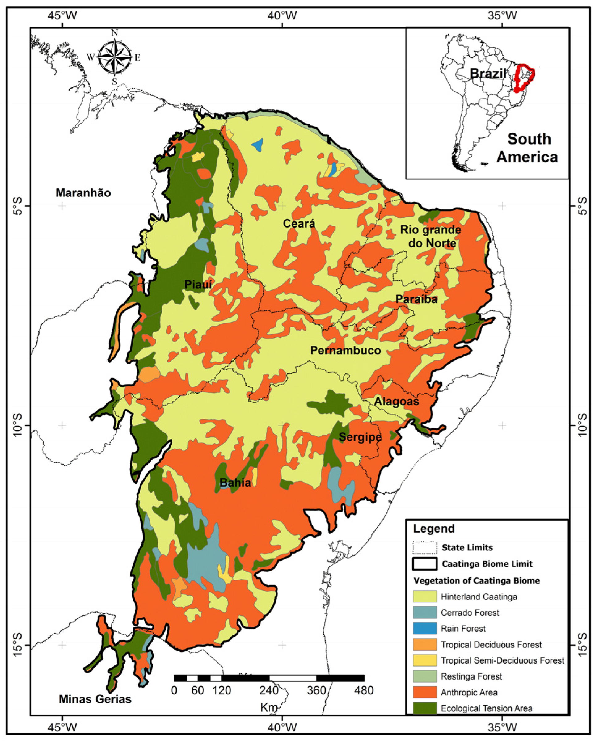
According to the Köppen–Geiger climate classification map published by Beck et al. [25], the study area mainly encompasses nine subtypes within three categories and its vegetation cover includes caatinga, rainforests, riparian forests, savannas, and montane forests, among others. Caatinga vegetation accounts for approximately 62% of NEB [26,27], with a rich diversity of vegetation types (Figure 2). The main plant species covered by Caatinga are Angico (Anadenanthera colubrina), Barriguda (Ceiba glaziovii), Cacto (Cactaceae), Carnaúba (Copernicia prunifera), Catingueira (Caesalpinia pyramidalis), Cumaru (Amburana cearensis), Facheiro (Pilosocereus pachycladus), and Juazeiro (Ziziphus joazeiro). These plant species withstand drought conditions and are used as food sources for humans and animals, and also play a crucial role in maintaining nutrient cycling within this biome [4]. Other climatic features of the study region are the annual mean rainfall of 400–800 mm, the annual average air temperature variation from 23 °C to 27 °C, and the potential evaporation (PET) of about 2000 mm year −1 [26].

2.2. Data Sources

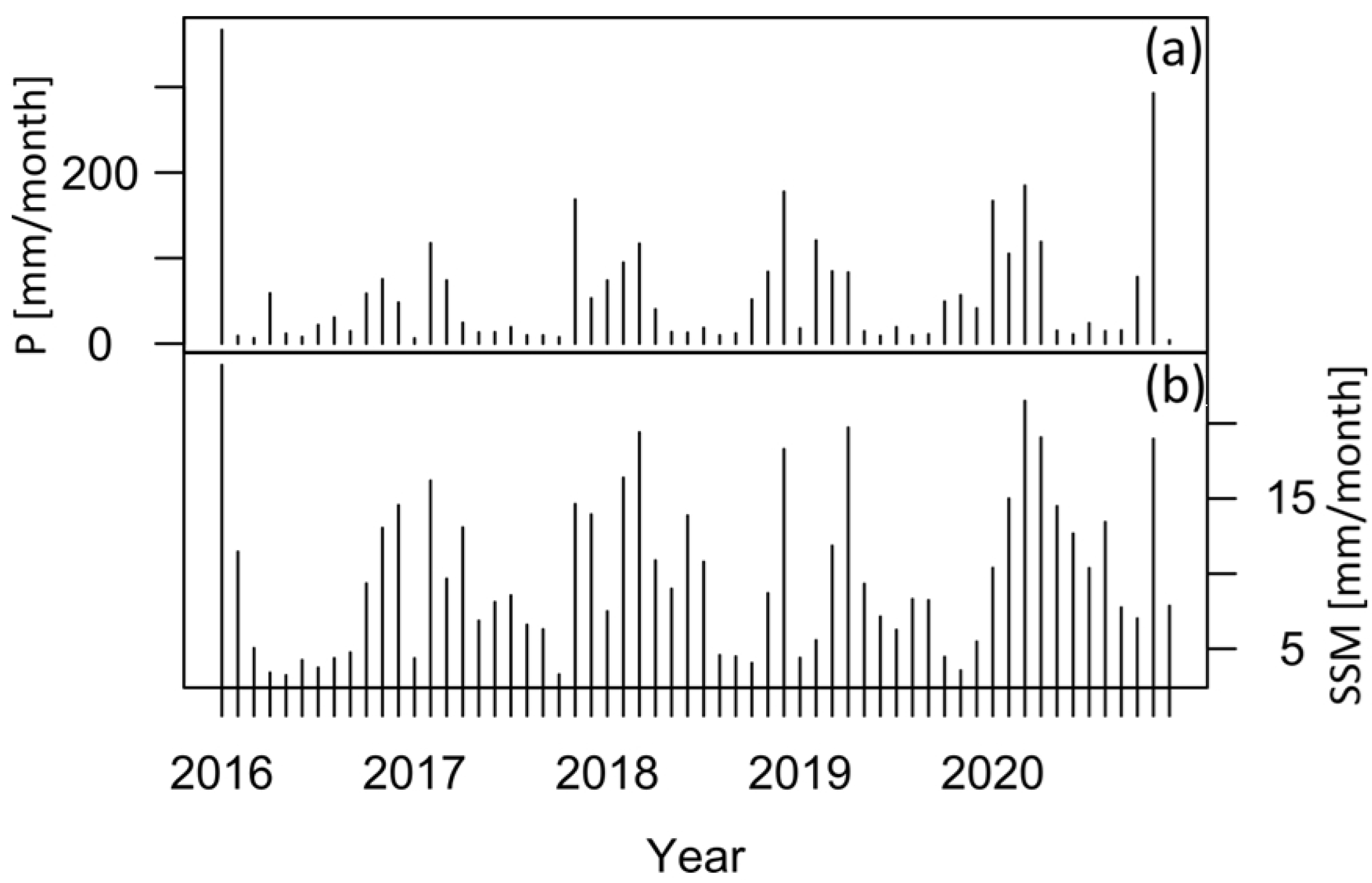
We obtained hydro-climatic data from the Brazilian Daily Weather Gridded Data (BR-DWGD) developed by Xavier et al. [28], a data product derived from a collection of algorithms and computer software designed to interpolate and extrapolate from daily meteorological observations to produce gridded estimates of daily weather parameters. The BR-DWGD were used to assess and identify periods of flash drought across northeastern Brazil from 2010 to 2022. The precipitation (P) and potential evapotranspiration (PET) variables shared a common spatial grid of 0.1° with daily data. The BR-DWGD variables used for this assessment were (P) precipitation and potential evapotranspiration (PET), at a common spatial grid of 0.1° on a daily scale. Therefore, referring to the calculation method of the Standardized Precipitation Evapotranspiration Index (SPEI), this study calculated the water deficit based on P and PET data in northeastern Brazil, fitted the water deficit data series using the log-logistic method [29], and used python tools to calculate SPEI data on a 3-month scale. Daily surface soil moisture (SSM) data were obtained from the SMOS L3 SSM product provided by the Barcelona Expert Center over the period of 2010–2022. An overview of the retrieved values is provided by González-Zamora et al. [30]. For example, the correlation between P and SSM portrays a linearity (Figure 3), which guarantees a physical relationship between the two variables.
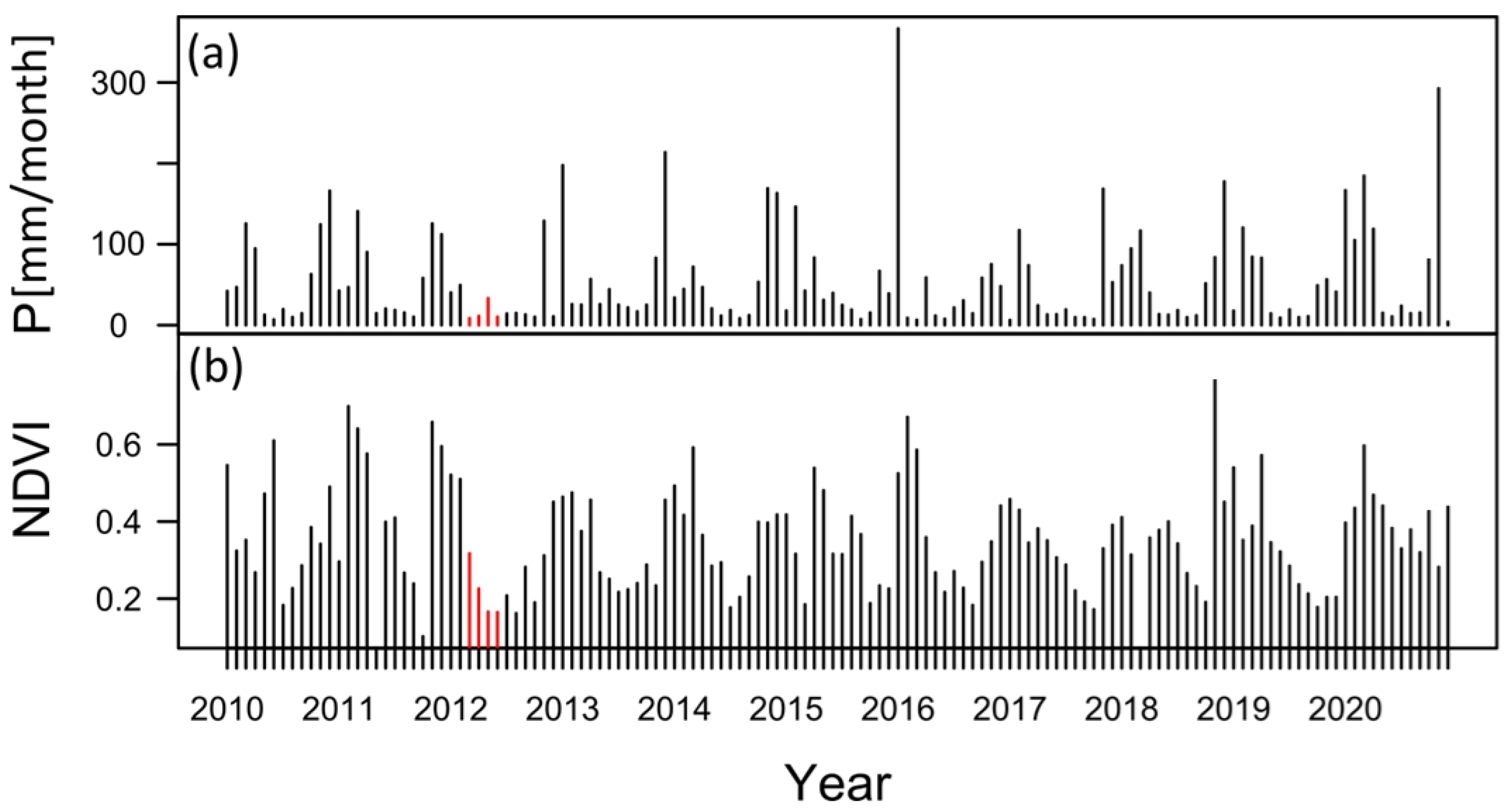
Daily NDVI data were provided by the Laboratory for Analyzing and Processing Satellite Images (LAPIS)’s archive [31], with a spatial resolution of 3 km. To synchronize the precipitation data’s temporal scales (Figure 4), we generated monthly and annual NDVI data series. Subsequently, all raster datasets were resampled to a 5 km resolution to facilitate analysis and discussion, and details of each data source are provided in Table 1. Previous studies have shown that the SPEI data from the BR-DWGD have a strong relationship with the soil moisture and vegetation response in NEB [27,28].
For testing, in addition to the soil moisture validation dataset described in Table 1, we also ensured all data were at are at the same spatial resolution and scale. NDVI data were resampled to a 10 km resolution using the bilinear interpolation method in GEE (Google Earth Engine). The spatial resolution of the NDVI data was about 3 km.

3. Methods

3.1. The Standardized Precipitation Evapotranspiration Index (SPEI)

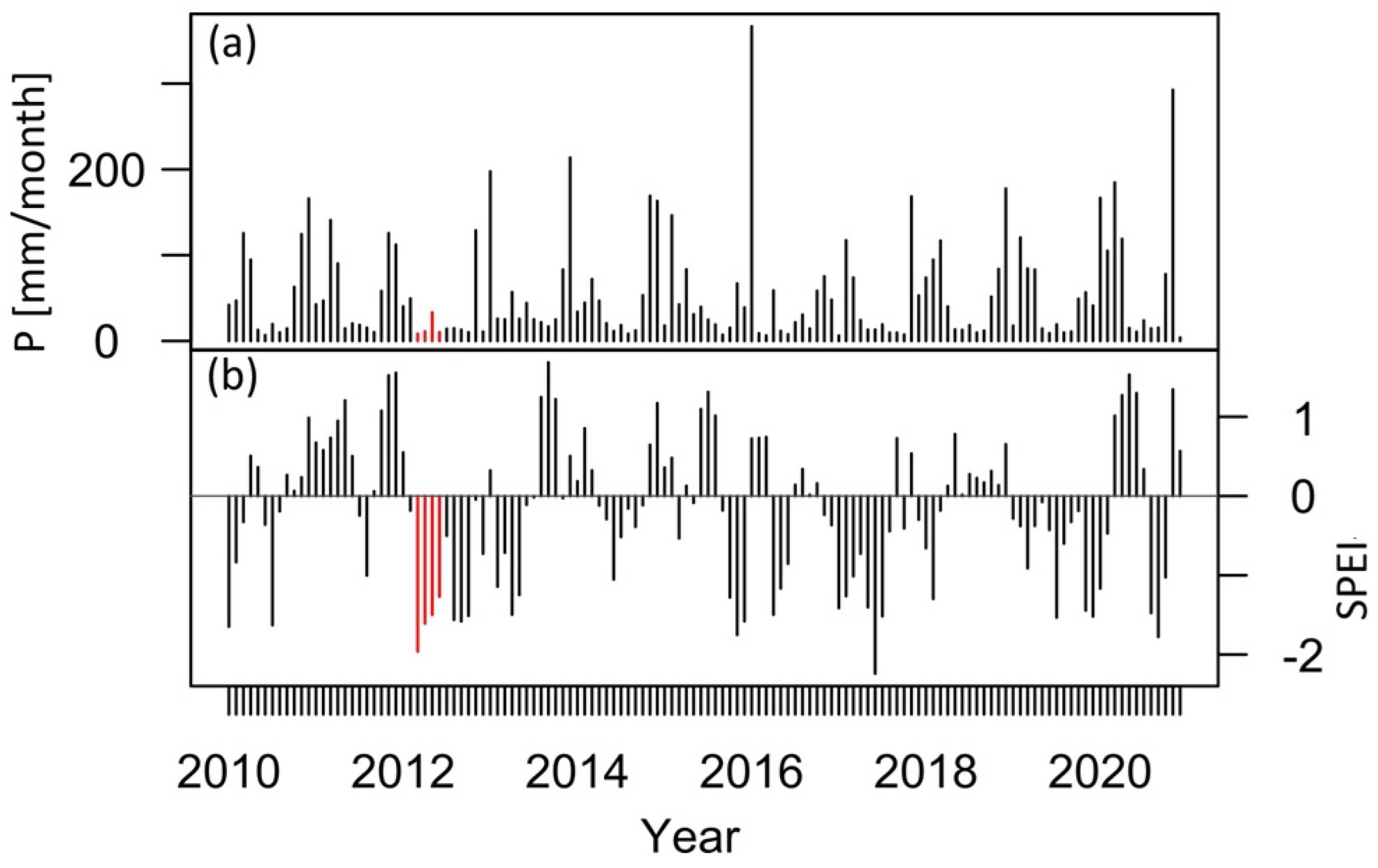
In this study, the SPEI was computed as a daily-scale drought index, which considers both P and PET from the BR-DWGD. The SPEI computation involves fitting the cumulative moisture deficit (D) series with an appropriate probability distribution function, followed by normalization to derive SPEI categories [29]. A log-logistic distribution was then used to fit the D time series [32]. Additionally, the Kolmogorov–Smirnov (K-S) test with a 0.05 significance level was used to determine the optimal probability distribution for northeastern Brazil using the gma library in Python. Negative SPEI values indicate water deficit, while positive values denote surplus moisture (Figure 5). We employed the log-logistic probability distribution function to fit D and conducted SPEI calculations for northeastern Brazil using the gma library in Python.
The PET is the sum of the amount of evaporation and transpiration from a reference vegetation of grass. It can be calculated with the Thornthwaite, Hargreaves, or Penman–Monteith equations [29]. The Thornthwaite equation is computed as follows:
PET = 16   ( L 12 ) ( N 30 ) ( 10 Td I ) α
α = ( 6.75   ×   10 7 ) I 3 ( 7.71   ×   10 5 ) I 2 + ( 1.792   ×   10 2 ) I + 0.49239
I = i = 1 12 ( Tmi 5 ) 1.514
where PET is the estimated potential evapotranspiration (mm/month), Td denotes the mean monthly temperature (degrees Celsius), N is the number of days for each month, L indicates the local insolation (hours/month), and I is the annual heat index, which depends on the monthly mean temperatures (Tmi in degrees Celsius).
We analyzed the correlations between the monthly hydro-climatic variables’ time series spanning from 2010 to 2022 and the SPEI sequence with various offsets (e.g., 0 months, 1 month, 2 months, and 3 months) over the study area. Utilizing an area-averaged time series of grid-scale R calculations, we detrended each variable to evaluate its response to drought (SPEI). Then, utilizing the maximum value, we identified the optimal response correlation for each variable and its corresponding lag intensity, employing a significance level of 95%. Subsequently, we applied a wavelet squared coherence analysis to reveal underlying oscillation patterns and changes in periodicities in a time–frequency domain between the area-averaged values of the SPEI against the SSM during their common time periods.

3.2. Model

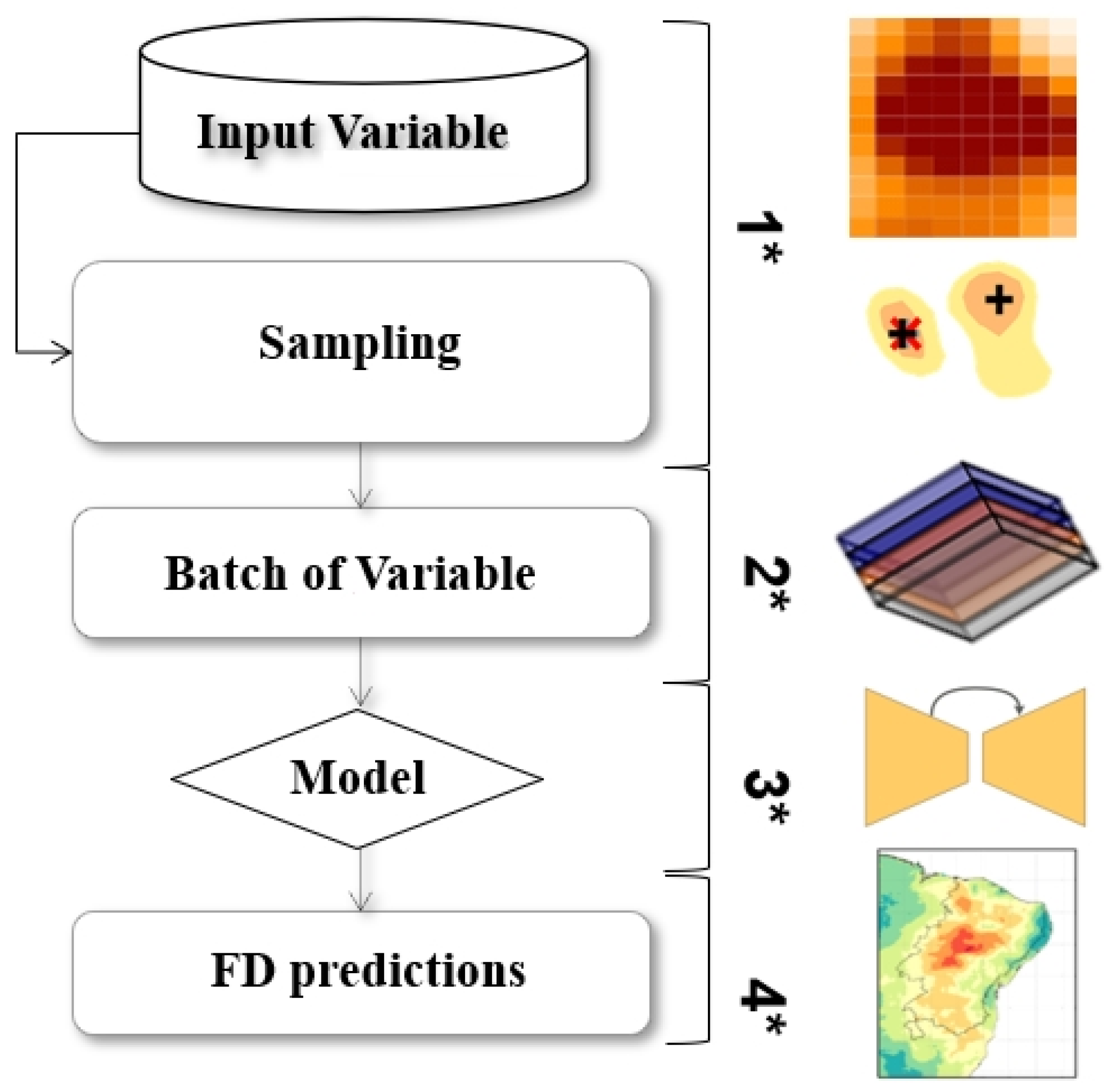
The processing pipeline of the model is illustrated in Figure 6. First, given a set of hydro-climatic variables, we select spatial data for northeastern Brazil. During training, we select variable data around drought events (further details in Section 3.4). The resulting batch of selected variable defines the sample to feed the model. Then, a Spatial Convolutional Encoder–Decoder (S-CED) architecture processes this sample by extracting relevant SSM information (encoder) and transforming it into a probabilistic drought detection map through time (decoder). During training, the resulting map is compared with the ground truth map for drought detection to define the penalty by which the model is optimized. Later, the drought detection map through time is provided for the entire area of study by concatenating the sample in the sequential order it was taken. Adding convolutions to neural networks promotes two biases in the model: (i) nearby pixels (locations) are related to each other, and (ii) targets can appear anywhere in the input data [29].
The convolutional neural networks (CNNs) model can yield acceptable accuracy for classifying well-known types of extreme weather events. Further, it has been gradually applied to the study of drought construction because it can effectively deal with the nonlinear relationship between various drought factors [17]. This is consistent with what others have observed. Wei and Li [21] found that the overall performance of deep learning is comparable to that of a random forest, and its multi-layer method can find the best output in the case of high-dimensional data features. However, the pooling layer of the CNN model leads to the loss of some important features during training, which may be one of the reasons why the accuracy of the training model is lower than that of the random forest model.

3.3. Model Architecture Design

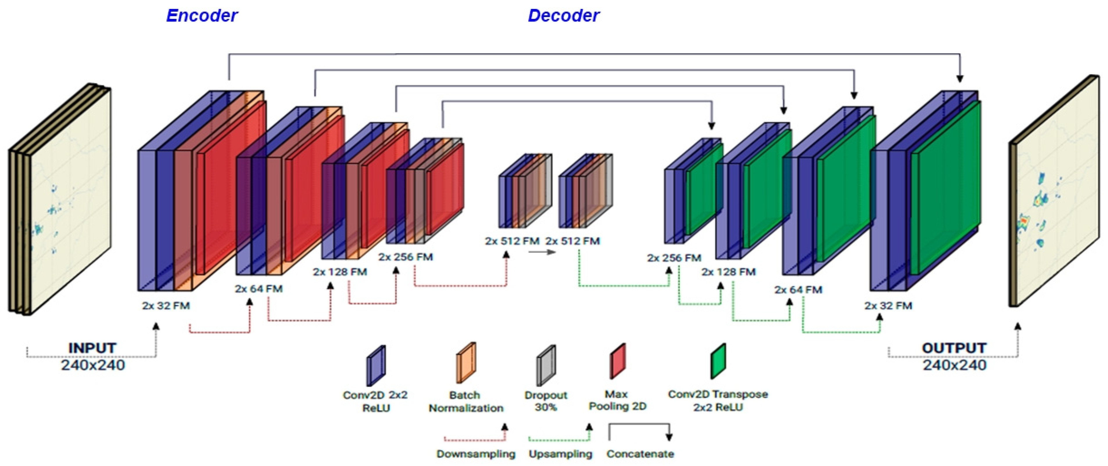
Detecting an FD requires network architectures capable of learning complex representations and exploiting interconnections in space and time. Adding convolutions to neural networks encourages two biases in the model: (i) nearby pixels (locations) are related to each other, and (ii) targets can appear anywhere in the input image [29]. Using convolutions significantly reduces the number of learnable parameters, resulting in faster learning and more scalable networks for deployment in real-case scenarios. Motivated by these properties, we propose an encoder–decoder architecture [33] that uses 2D convolutional layers to process hydro-climatic variables in space for FD detection as a binary classification task (FD vs. non-drought conditions) at the grid level. The splits are defined such that the amount of flash drought grids in each is similar, with the corresponding drought vs. non-drought ratios being 0.8%, excluding water. In a nutshell, the network receives as input a batch of data variables of size (lat, lon), with lat and lon being the latitude and longitude sizes, respectively. The model comprises two 2D convolutional layers for the encoder and two corresponding 2D convolutional layers for the decoder. CNNs utilize layers of convolutional filters to automatically detect and learn hierarchical patterns and features from the input data. Due to a reduction in the number of learnable parameters, deep learning offers high accuracy and efficiency in processing large datasets [34,35]. The architecture is shown in Figure 7.
The model uses a batch normalization, a normalization layer, a modified linear unit layer (ReLU), and a fully connected layer. At the encoder, max pooling is used after dropout layers to reduce the spatial dimensions by a factor of two. Likewise, residual skip connections [35,36] connect the encoder and the decoder blocks. At the top of the decoder, a final 2D convolutional layer followed by a sigmoid activation produces the class probabilities for each pixel, which constitute FD detection maps through time. In this study, we present the selected hydro-climatological data of size (240, 240) and output the probabilistic drought detection map of size (240, 240). Convolutional layers typically employ padding to extend the range of the convolution operation at image borders and produce an output that is the same size as the input [16,37]. Using valid convolutions has the noticeable caveat that each convolution produces feature maps with fewer elements. In a nutshell, the network receives as input a batch of selected data of variable size (lat, lon), with lat and lon being the latitude and longitude sizes, respectively. The model comprises 2D convolutional layers for the encoder and two corresponding 2D convolutional layers for the decoder. Exploiting convolutions significantly reduces the number of learnable parameters, resulting in faster learning and more scalable networks for deployment in real-case stages.

3.4. Flash Drought Identification

FDs were identified over the period 2010–2022 using SPEI and SSM values. The SPEI was spatially averaged for the study area. To enhance the accuracy of FD identification, the five-day average of the SSM time series was taken. The daily SPEI can exhibit noise due to short-term meteorological variability that can potentially obscure the FD onset [14,38]. By averaging the SPEI values over five-day intervals, the variability was mitigated while still being sufficient to capture the rapid intensification period characteristic of FDs. Flash drought events were identified using multi-criterion guidelines as defined in previous studies [4]. This method employs the following criteria: (1) the total decrease in the SPEI should be 2 or greater in a 30-day period; (2) at the end of the same 30-day period, the SPEI value should be less than −1.5 (or the SSM should be below the 20th percentile); and (3) after crossing the drought threshold value of −0.5, the SPEI should remain below −0.5 for at least 30 days. The first criterion captures the rapid intensification aspect of FDs and confirms that the identified events are not affected by temporary fluctuations in the SPEI or SSM due to increased rainfall, decreased temperatures, or increased cloud cover. The second and third criteria help separate FDs and dry spells and identify flash drought events that may have potential environmental impacts over more extended periods. The SSM is expressed in a percentage format. The daily values of the SSM data are assigned to different percentile categories of FDs, including 20th–25th, 15th–20th, 10th–15th, and <10th (Table 2). The quantile values provide a useful way of comparing the SPEI with varying orders of magnitude. They help to standardize the data and make them easier to compare and analyze FD categories across different regions. Although drought categories are binary, i.e., drought/non-drought, we rely on the assumption that the FD detection system should be continuous and capture the evolution of the phenomena. This is achieved by taking the probability distribution by which an example is labeled as belonging to one category and not to another (i.e., the similarity structure), as shown in Table 2.
Furthermore, the Coupled Model Intercomparison Project Phase 6 (CMIP6) was used to calculate the SPEI3 for identifying future stages of FD based on the SPEI under a high-emission scenario. The following variables were employed: water evapotranspiration flux, maximum air temperature, minimum air temperature, and precipitation. These data were derived from historical simulations and Shared Socioeconomic Pathways (SSPs) that characterize four future scenarios; we chose to use the SSP5-8.5 of CMIP6. The historical simulation data cover the period from 2010 to 2015, while the data for the future scenario cover the period from 2024 to 2050. We used the NorESM Climate Modeling Consortium (NCC) agency, which has a spatial resolution of 1.25°.

4. Results

4.1. Evaluation of Hydro-Climatic Data in Response to Drought

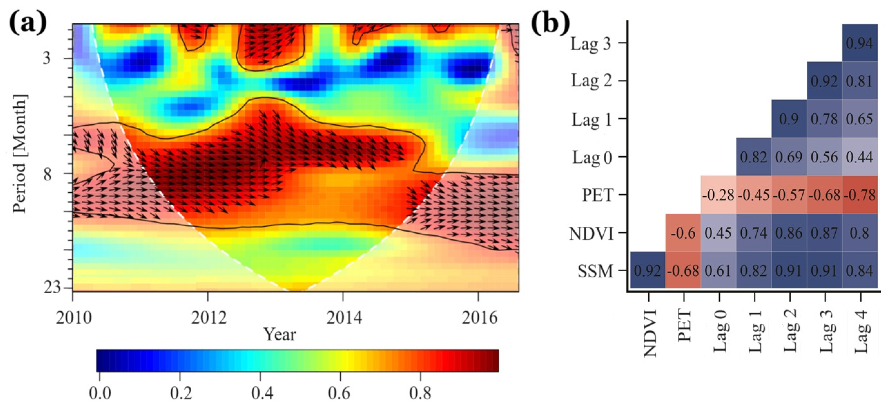
In the analysis of wavelet coherence between the SPEI and SSM (Figure 8a), it is evident that the periodicity of 8–12 months is predominantly high from 2010 to 2016 (significant at a 95% level). The cone area denotes the cone of influence under which the period (month) can be considered for the analysis. Hence, it is evident from the wavelet analysis that the SPEI changes are in accord with the different periodicities of the SSM, which are also interpreted as drought-induced temporal effects on the SSM over NEB. Considering that the SPEI has a stronger explanatory power on the intensity of drought, which includes information on temperature, precipitation, and potential evapotranspiration, this study selected the SSM, NDVI, and PET as independent hydro-climate variables.
Figure 8b reflects the interactive effects of each variable on the temporal impact of drought (SPEI). The SSM and NDVI dominate as the driving factors, followed by the PET. We identified the lag effect durations of each variable during drought as follows: SSM > NDVI > PET. In addition, we observed significant negative correlations between the PET and drought, indicating a stronger response of the PET to lagging drought (i.e., higher sensitivity). Longer lag effect times imply that the SSM is more likely to be affected by the lingering effects of previous months’ droughts and is less likely to recover from earlier droughts. Compared to other commonly used meteorological drought indices, the SPEI exhibits a greater capability to measure the impacts of drought on agricultural and ecological responses [27,29]. Thus, we conclude that the SSM was the optimal variable for drought detection.

4.2. Identifying and Mapping Flash Drought Events

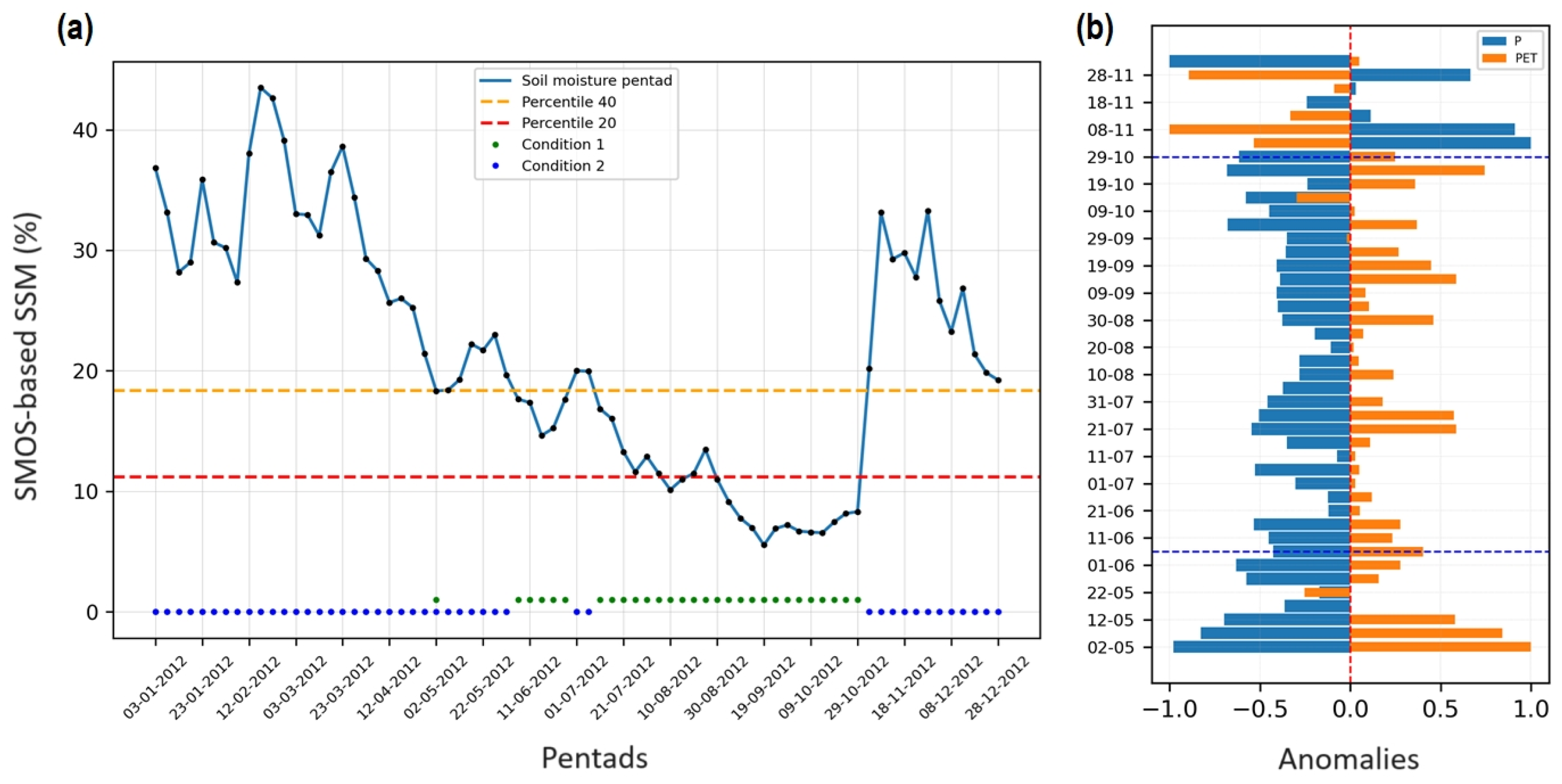
To showcase the ability of the SSM to capture FDs, the well-studied 2012 NEB event was examined. This drought event occurred during the autumn, winter, and spring of 2012 and was a historically unprecedented event in NEB, ranked as the third-largest drought in terms of aerial extent since 1901. The event was preceded by La Niña conditions during the summers of 2011–2012, resulting in drier-than-normal conditions at the beginning of the year [26,31]. Figure 9 shows the rapid onset and progression of the 2012 flash drought demonstrated by SSM values every 5 days (i.e., pentads) from 1 March to 28 December. The drought reached its peak severity at the end of August, with nearly three-fourths of NEB classified as having severe or extreme drought conditions according to the SPEI categories. The mean and median lengths of the flash drought events in 2012 were 24 and 114 days. This indicates that the flash drought events identified in NEB lasted approximately 1–4 months.
By examining Figure 9, we see that the minimum SSM values were experienced in August–October, reaching less than the 10th percentile. The synchronization of the P and PET during the onset of the 2012 flash drought highlights the connection between the onset of flash drought conditions indicated by the SSM and subsequent reductions in precipitation, offering insights into the linked dynamics of the atmospheric and hydrological responses.
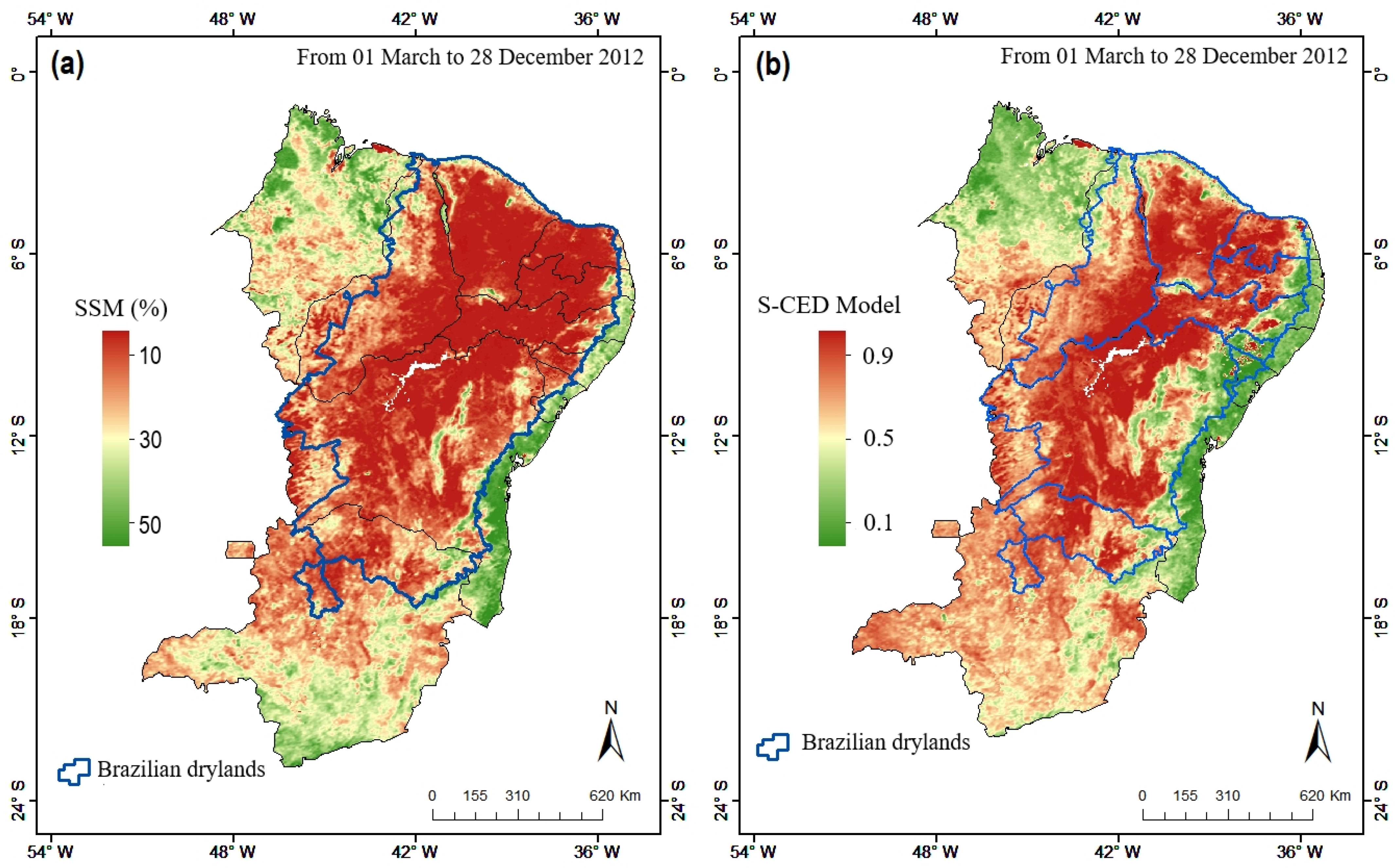
The analysis of FD events in 2012 within NEB reveals variations in the visual comparative analysis between SMOS-based SSM retrievals and the CNN model simulation. The employed criteria ensured robust identification of FDs by considering the multi-criterion approach outlined in Section 3.4. Figure 10 shows the five-day averages of the SSM and CNN from 1 March to 28 December 2012. Each map is represented by a mean grid-point (pixel level), with red indicating instances where the SSM caused an FD, and green indicating non-drought locations. Non-drought conditions fall within typical hydro-climatic conditions and are comparable to easy-to-classify locations. Moreover, FDs have various stages in their development, as shown in Figure 9a.
We provide a visual comparison of the performance of the S-CED model trained with the SSM and SMOS L3 SSM product. First, in Figure 10, we present the northeastern Brazil probabilistic drought detection map provided by the S-CED model during the 2012 FD events. A more intense red color in the S-CED model corresponds to higher scores. This visualization is used to identify the model’s distribution results of all the grids in the study region compared to soil moisture conditions estimated from the SSM product. The red areas in the maps delimit the areas of flash drought events identified for the region, and a green colormap is used to represent the non-drought category. Thus, the probabilistic scores of the S-CED model in non-drought category areas (the green color) are higher than those obtained by the SSM product. The blue contours encompass the Brazilian drylands, where the visual accuracy is higher between two maps. We also obtain clear signals of potential non-droughts, highlighting the usefulness of the proposed model and the benefits of the method for flash drought identification.
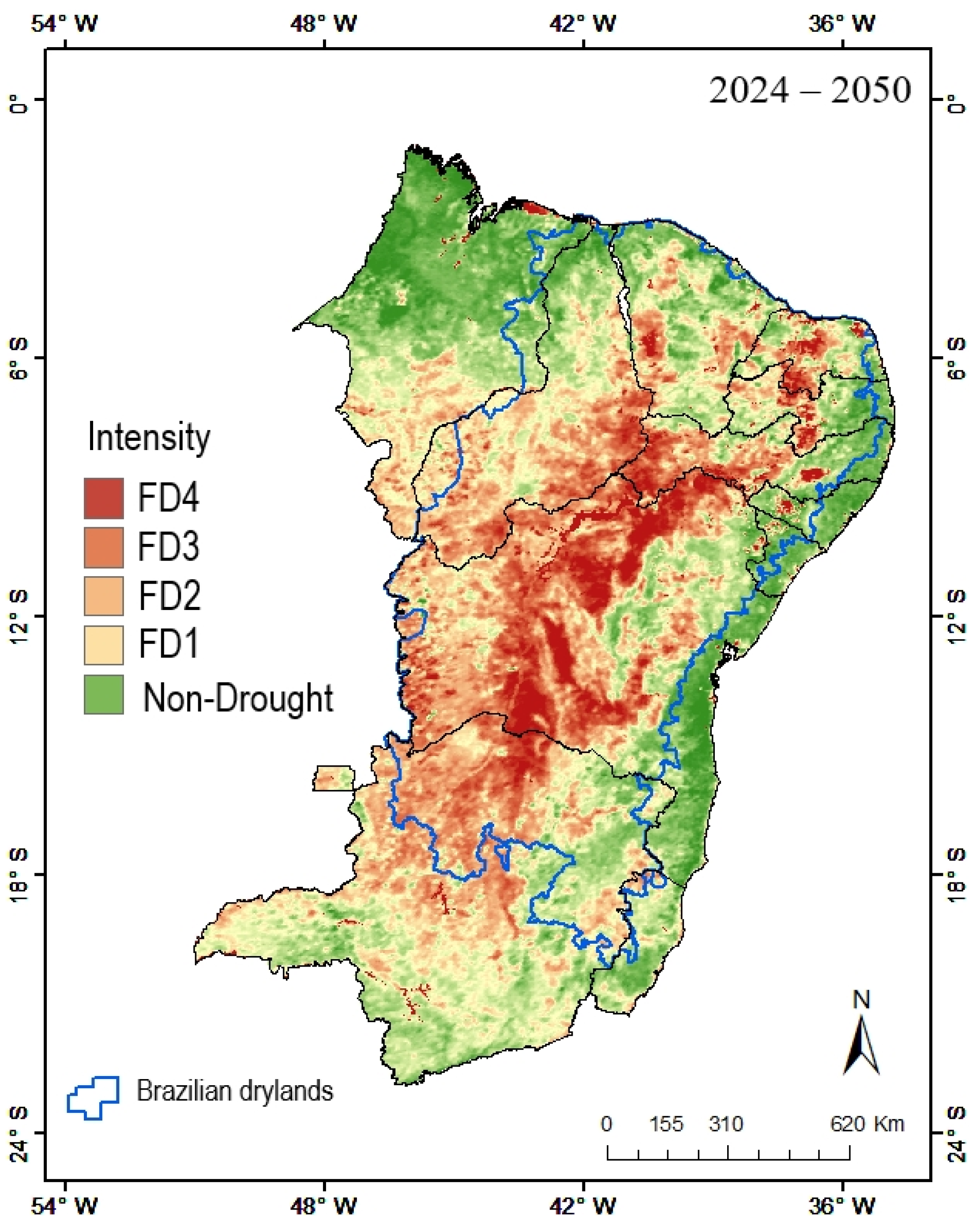
FD events were identified in the growing season (February–May) from 2024 to 2050 within NEB using the CMIP6 predictions. Our focus was on capturing the FD events to better comprehend their impact on the main rainy season of NEB. Figure 11 shows the intensity (percentile/year) of FDs in the SSP5-8.5 scenario. The primary impact is primarily concentrated in the São Francisco River Basin, within NEB’s semi-arid region. The entire basin is engulfed in FD conditions, characterized by increased severity in its central region, where the dominant FD4 and FD3 are observed. These categories indicate the severity of FD conditions, which are close to the extreme drought category defined by the SPEI, and pose significant challenges to water resources, agriculture, and ecosystems within those areas. Additionally, the results revealed the FD intensity, showing that 28% of the region was categorized as FD1. FD2 accounted for 23%, while FD3 and FD4 comprised 21% of the NEB-FD area. It indicates that NEB’s semi-arid region (i.e., the Caatinga biome) will face significant challenges in terms of FD risk under future scenarios. Therefore, understanding the interconnected nature of water management within the entire basin is crucial for comprehensively assessing and addressing the impacts of severe flash droughts in those areas.

5. Discussion

We present a new method for FD identification using different types of input data. An FD is a rapid drought in a short period caused by severe heat waves and rainfall deficiency [4,25]. It is very difficult to accurately detect an FD [7,12]. The occurrence of an FD is related to the complex interaction of soil moisture, evapotranspiration, and vegetation. This research adopts the CNN architecture for FD identification to output data from model simulations in northeastern Brazil (NEB) by integrating multiple sources of hydrometeorological data that represent the atmosphere (P and PET data), surface (NDVI data), and subsurface (SSM data). We selected SSM data to train the proposed model using a cross-correlation analysis and tried to avoid splitting the responses of multiple drought types. The complete area was divided into data of the same size as the samples used for training, and the model generated probabilistic scores for surface soil moisture data. These scores were then used to reconstruct the entire region.
The method-based neural representation has been applied in northeastern Brazil, and it can identify an FD after training with SSM data. The comparison against outcomes from the CNN model implementation reveals a slight increase in its capability to properly identify FD areas, which is more substantial when forcing the algorithm with surface soil moisture. Examination of the CNN’s ability to effectively capture FD events revealed its proficiency in identifying the development phase. The spatial mapping of the 2012 FD showcased variations in intensity across NEB, with distinct patterns in different regions. The southwest NEB region experiences frequent FDs, while the northeast encounters less frequent events, and its semi-arid region faces severe FD conditions. Additionally, our study underscores the lag effects of drought on different environmental factors, enriching our comprehension of soil moisture’s response to drought. The delayed response emphasized the complex relationship between meteorological and hydrological factors during FD events, highlighting the challenge of predicting and mitigating the consequences of FDs on the NEB drylands.
The NEB drought events of 2012 showed an evident accuracy in the spatial domain, as shown in Figure 7. The soil moisture dataset from satellite observations is at the root of it. We can see how the learned models obtain distinctive simulations for the registered FD events. We also find clear signals of potential unregistered droughts, highlighting the usefulness of the proposed model and the benefits of the method for drought detection. CNNs offer high accuracy and efficacy in processing large datasets, though they may lose some features due to pooling layers, slightly lowering the accuracy compared to the random forest model [39].
We found that the model had enough representational capacity with two layers for the encoder and two for the decoder. More layers decreased the performance results for the validation data. Convolutional layers typically employ padding to extend the range of the convolution operation at image borders and produce an output that is the same size as the input [39,40]. Multiple values for the padding exist, with the zero-valued one being the most common. However, padding introduces artificial distortions that do not align with the actual behavior of hydro-climatological variables. As such, we refrained from using padding in the convolutions and performed valid convolutions. Using valid convolutions has the noticeable caveat that each convolution produces feature maps with fewer elements.
Nevertheless, uncertainties persist. Comparing the CNN with the surface soil moisture provided a holistic perspective on the interconnected dynamics during FD events. The synchronization observed between the severity of FD conditions indicated by the CNN and subsequent reductions in soil moisture highlighted the potential of our proposed approaches to improve FD detection algorithms. The uncertainty and bias in the SSM data are at the root of unregistered FD events. We acknowledge that validating the model under categories of drought and non-drought settings is challenging since these problems also affect the validation data. This can lead to poor estimation of generalization capabilities and wrongly tuned models [41]. Since the number of drought and non-drought grids varies considerably, we balanced their contribution by computing a correction factor for each location based on [41].
By leveraging the CMIP6 (SSP5-8.5) as a predictive tool, our findings revealed that the FD severity in the São Francisco River Basin within NEB will increase in the future due to higher persistent dry conditions associated with global warming. In general, an expansion of the area under FD events in the context of high-emission scenarios was observed the middle and south areas of the basin from 2024 to 2050 (Figure 11). By examining Figure 11, we see that a wide range of minimum SPEI values are observed across NEB, spanning from 0.99 to <−2.00 (see Table 1). These values indicated the severity of flash drought conditions, with lower SPEI values representing more intense flash droughts (FD4). NEB’s areas with minimum SPEI values higher than −2.00 are likely to experience more extreme flash drought events, posing significant challenges to water resources, agriculture, and ecosystems within those areas.
Nevertheless, as shown in Figure 11, the high dependence of the NEB rainy season (February–May) on weather conditions with insufficient rainfall has raised concern about the risk climate change poses to the entire regional economy [26]. These concerns are even greater since climate change projections suggest that future flash droughts will be more severe. In the context of the growing season, agricultural activities that are dependent on consistent water availability face disruptions that can impact crop yields and overall food production [23]. Changes in plant growth and transpiration due to climate change will have a direct impact on watershed processes, potentially leading to an increased intensity of drought conditions in the São Francisco River Basin in northeastern Brazil [26]. However, because of the uncertainties in the independent climate models of CMIP6, multi-model ensembles were typically used to minimize the impact of the models’ uncertainties in the prediction results.

6. Conclusions

Flash drought (FD) detection and its prediction is of utmost importance in the present scenario because of its increase due to climate change. Our research introduces a novel methodology based on a deep learning model which, after training, can identify an FD. This process embeds spatiotemporal FD-identifying thresholds into the process of generating probabilistic scores from models that are trained with surface soil moisture data. In conclusion, the goals of the study were met by introducing a 2D convolutional encoder–decoder architecture and integrating multiple sources of hydro-climatic data to identify the complexity of spatial FD events across northeastern Brazil. As flash droughts pose challenges to accurate detection due to their complex spatial–temporal features, the insights gained from this research provide a foundation for further studies.

Author Contributions

H.A.B., methodology, formal analysis, investigation, writing—original draft, visualization, conceptualization, funding acquisition, and project administration. C.O.B., conceptualization, writing—review, and editing. T.V.L.K., writing—review and editing. All authors have read and agreed to the published version of the manuscript.

Funding

This study was supported by the Coordenação de Aperfeiçoamento de Pessoal de Nível Superior (CAPES 01/2022), Brazil, under the Project No. 88881.7050501/2022-01 to H.A.B through PEPEEC (Programa Emergencial de Prevenção e Enfretamento de Desastres Relacionados a Emergências Climáticas, Eventos Extremos e Acidentes Ambientais). It also had the support of the CNPq under project No. 403223/2021-0 to H.A.B through the Desertification Monitoring Program in the Brazilian Semi-arid Region.

Institutional Review Board Statement

Not applicable.

Informed Consent Statement

Not applicable.

Data Availability Statement

Publicly available datasets were analyzed in this study. This data can be found here: https://www.lapismet.com.br.

Acknowledgments

The authors are grateful for the comments from three reviewers who helped to significantly improve the quality of the manuscript. The authors offer thanks for the use of the European Weather Cloud (EWC) for providing processing capabilities for large data.

Conflicts of Interest

The authors declare that they have no known competing financial interests or personal relationships that could have appeared to influence the work reported in this paper.

References

  1. Wilhite, D.A. Chapter I Drought as a Natural Hazard: Concepts and Definitions; Drought A Glob. Assess; Drought Mitigation Center Faculty Publications: Lincoln, NE, USA, 2000. [Google Scholar]
  2. Cook, B.I.; Mankin, J.S.; Anchukaitis, K.J. Climate Change and Drought: From Past to Future. Curr. Clim. Chang. Rep. 2018, 4, 164–179. [Google Scholar] [CrossRef]
  3. Wu, C.; Ning, S.; Jin, J.; Zhou, Y.; Zhou, L.; Bai, X.; Zhang, L.; Cui, Y. Construction and application of comprehensive drought index based on uncertainty cloud reasoning algorithm. Sci. Total Environ. 2021, 779, 146533. [Google Scholar] [CrossRef]
  4. Barbosa, H.A. Understanding the rapid increase in drought stress and its connections with climate desertification since the early 1990s over the Brazilian semi-arid region. Arid Environ. 2024, 222, 105142. [Google Scholar] [CrossRef]
  5. Ahmad, S.K.; Kumar, S.V.; Lahmers, T.M.; Wang, S.; Liu, P.-W.; Wrzesien, M.L.; Bindlish, R.; Getirana, A.; Locke, K.A.; Holmes, T.R.; et al. Flash Drought Onset and Development Mechanisms Captured with Soil Moisture and Vegetation Data Assimilation. Water Resour. Res. 2022, 58, e2022WR032894. [Google Scholar] [CrossRef]
  6. Lisonbee, J.; Woloszyn, M.; Skumanich, M. Making sense of flash drought: Definitions, indicators, and where we go from here. J. Appl. Serv. Climatol. 2021, 2021, 1–19. [Google Scholar] [CrossRef]
  7. Svoboda, M.; LeComte, D.; Hayes, M.; Heim, R.; Gleason, K.; Angel, J.; Rippey, B.; Tinker, R.; Palecki, M.; Stooksbury, D.; et al. THE DROUGHT MONITOR. Bull. Am. Meteorol. Soc. 2022, 83, 1181–1190. [Google Scholar] [CrossRef]
  8. Yuan, X.; Ma, F.; Li, H.; Chen, S. A review on multi-scale drought processes and prediction under global change. Trans. Atmos. Sci. 2020, 43, 225–237. [Google Scholar]
  9. Mukherjee, S.; Mishra, A.K. A Multivariate Flash Drought Indicator for Identifying Global Hotspots and Associated Climate Controls. Geophys. Res. Lett. 2022, 49, 2. [Google Scholar] [CrossRef]
  10. Ji, Y.; Fu, J.; Lu, Y.; Liu, B. Three-dimensional-based global drought projection under global warming tendency. Atmos. Res. 2023, 291, 106812. [Google Scholar] [CrossRef]
  11. Xu, Y.; Zhang, X.; Hao, Z.; Hao, F.; Li, C. Projections of future meteorological droughts in China under CMIP6 from a three-dimensional perspective. Agric. Water Manag. 2021, 252, 106849. [Google Scholar] [CrossRef]
  12. Zargar, A.; Sadiq, R.; Naser, B.; Khan, F.I. A review of drought indices. Environ. Rev. 2011, 19, 333–349. [Google Scholar] [CrossRef]
  13. Zhou, S.; Williams, A.P.; Berg, A.M.; Cook, B.I.; Zhang, Y.; Hagemann, S.; Lorenz, R.; Seneviratne, S.I.; Gentine, P. Land–atmosphere feedbacks exacerbate concurrent soil drought and atmospheric aridity. Proc. Natl. Acad. Sci. USA 2019, 116, 18848–18853. [Google Scholar] [CrossRef]
  14. Zhang, Q.; Shi, R.; Singh, V.P.; Xu, C.Y.; Yu, H.; Fan, K.; Wu, Z. Droughts across China: Drought factors, prediction and impacts. Sci. Total Environ. 2022, 803, 150018. [Google Scholar] [CrossRef]
  15. Quiring, S.M.; Ford, T.W.; Wang, J.K.; Khong, A.; Harris, E.; Lindgren, T.; Goldberg, D.W.; Li, Z. The north American soil moisture database development and applications. Bull. Am. Meteorol. Soc. 2016, 97, 1441–1460. [Google Scholar] [CrossRef]
  16. Chattopadhyay, A.; Hassanzadeh, P.; Pasha, S. Predicting clustered weather patterns: A test case for applications of convolutional neural networks to spatio-temporal climate data. Sci. Rep. 2020, 10, 1317. [Google Scholar] [CrossRef]
  17. Reichstein, M.; Camps-Valls, G.; Stevens, B.; Jung, M.; Denzler, J.; Carvalhais, N.; Prabhat, F. Deep learning and process understanding for data-driven earth system science. Nature 2019, 566, 195–204. [Google Scholar] [CrossRef]
  18. Camps-Valls, G.; Tuia, D.; Zhu, X.X.; Reichstein, M. Deep Learning for the Earth Sciences: A Comprehensive Approach to Remote Sensing, Climate Science and Geosciences; John Wiley & Sons: Hoboken, NJ, USA, 2021. [Google Scholar]
  19. Vandal, T.; Kodra, E.; Ganguly, S.; Michaelis, A.; Nemani, R.; Ganguly, A.R. Generating high resolution climate change projections through single image super-resolution: An abridged version. IJCAI Int. Jt. Conf. Artif. Intell. 2018, 5389–5393. [Google Scholar] [CrossRef]
  20. Gibson, P.B.; Chapman, W.E.; Altinok, A.; Monache, L.D.; DeFlorio, M.J.; Waliser, D.E. Training machine learning models on climate model output yields skillful interpretable seasonal precipitation forecasts. Commun. Earth Environ. 2021, 2, 159. [Google Scholar] [CrossRef]
  21. Wei, T.; Li, Y.F. Does tail label help for large-scale multi-label learning? IEEE Trans. Neural Netw. Learn. Syst. 2020, 31, 2315–2324. [Google Scholar]
  22. IBGE Instituto Brasileiro de Geografia e Estatística. População. Estados. Rio de Janeiro. IBGE 2023. Available online: http://censo2023.ibge.gov.br/apps/atlas/ (accessed on 20 April 2024).
  23. Marengo, J.A.; Torres, R.R.; Alves, L.M. Drought in Northeast Brazil-past, present, and future. Theor. Appl. Climatol. 2017, 129, 1189–1200. [Google Scholar] [CrossRef]
  24. Barbosa, H.A. Flash drought and its characteristics in northeastern South America during 2004–2022 using satellite-based products. Atmosphere 2023, 14, 1629. [Google Scholar] [CrossRef]
  25. Beck, H.E.; McVicar, T.R.; Vergopolan, N.; Berg, A.; Lutsko, N.J.; Dufour, A.; Zeng, Z.; Jiang, X.; van Dijk, A.I.J.M.; Miralles, D.G. High-resolution (1 km) Köppen-Geiger maps for 1901–2099 based on constrained CMIP6 projections. Sci. Data 2023, 10, 724. [Google Scholar] [CrossRef]
  26. Buriti, C.; Humberto, A.B.; Franklin, P.; Kumar, T.V.L.; Manoj, K.T.; Koteswara, R. Un siglo de sequías: ¿por qué las políticas de agua no desarrollaron la región semiárida brasileña? Rev. Bras. De Meteorol. 2020, 35, 683–688. [Google Scholar] [CrossRef]
  27. Giovannettone, J.; Franklin, P.; Humberto, B.A.; Carlos, A.C.; Kumar, T.V.L. Characterization of links between hydro-climate indices and long-term precipitation in Brazil using correlation analysis. Int. J. Climatol. 2020, 40, 5527–5541. [Google Scholar] [CrossRef]
  28. Xavier, A.C.; Scanlon, B.R.; King, C.W.; Alves, A.I. New improved Brazilian daily weather gridded data (1961–2020). Int. J. Climatol. 2022, 42, 8390–8404. [Google Scholar] [CrossRef]
  29. Vicente-Serrano, S.M.; Beguería, S.; Lopez-Moreno, J.I. A multiscalar drought index sensitive to global warming: The Standardized Precipitation Evapotranspiration Index. J. Clim. 2010, 23, 1696–1718. [Google Scholar] [CrossRef]
  30. González-Zamora, Á.; Sánchez, N.; Martínez-Fernández, J.; Gumuzzio, Á.; Piles, M.; Olmedo, E. Long-term SMOS soil moisture products: A comprehensive evaluation across scales and methods in the Duero Basin (Spain). Phys. Chem. Earth Parts A/B/C 2015, 83–84, 123–136. [Google Scholar] [CrossRef]
  31. Barbosa, H.A.; Lakshmi Kumar, T.V. Influence of rainfall variability on the vegetation dynamics over Northeastern Brazil. J. Arid Environ. 2016, 124, 377–387. [Google Scholar] [CrossRef]
  32. Stagge, J.H.; Tallaksen, L.M.; Gudmundsson, L.; Van Loon, A.F.; Stahl, K. Candidate distributions for climatological drought indices (SPI and SPEI). Int. J. Climatol. 2015, 35, 4027–4040. [Google Scholar] [CrossRef]
  33. Sun, T.; Ferreira, V.; He, X.; Andam-Akorful, S. Water Availability of São Francisco River Basin Based on a Space-Borne Geodetic Sensor. Water 2016, 8, 213. [Google Scholar] [CrossRef]
  34. Shen, R.; Huang, A.; Li, B.; Guo, J. Construction of a drought monitoring model using deep learning based on multi-source remote sensing data. Int. J. Appl. Earth Obs. Geoinf. 2019, 79, 48–57. [Google Scholar] [CrossRef]
  35. Ji, S.; Xu, W.; Yang, M.; Yu, K. 3d convolutional neural networks for human action recognition. IEEE Trans. Pattern Anal. Mach. Intell. 2012, 35, 221–231. [Google Scholar] [CrossRef]
  36. He, K.; Zhang, X.; Ren, S.; Sun, J. Deep residual learning for image recognition. In Proceedings of the 2016 IEEE Conference on Computer Vision and Pattern Recognition (CVPR), Las Vegas, NV, USA, 27–30 June 2016; pp. 770–778. [Google Scholar]
  37. Khosravi, K.; Panahi, M.; Golkarian, A.; Keesstra, S.D.; Saco, P.M.; Bui, D.T.; Lee, S. Convolutional neural network approach for spatial prediction of flood hazard at national scale of iran. J. Hydrol. 2020, 591, 125552. [Google Scholar] [CrossRef]
  38. He, M.; Kimball, J.S.; Yi, Y.; Running, S.; Guan, K.; Jensco, K.; Maxwell, B.; Maneta, M. Impacts of the 2017 flash drought in the US Northern plains informed by satellite-based evapotranspiration and solar-induced fluorescence. Environ. Res. Lett. 2019, 14, 074019. [Google Scholar] [CrossRef]
  39. Prodhan, F.A.; Zhang, J.; Hasan, S.S.; Pangali Sharma, T.P.; Mohana, H.P. A review of machine learning methods for drought hazard monitoring and forecasting: Current research trends, challenges, and future research directions. Environ. Model. Softw. 2022, 149, 105327. [Google Scholar] [CrossRef]
  40. Zhang, A.; Lipton, Z.C.; Li, M.; Smola, A.J. Dive into Deep Learning; Cambridge University Press: Cambridge, UK, 2023. [Google Scholar]
  41. Lawrence, S.; Burns, I.; Back, A.; Tsoi, A.C.; Giles, C.L. Neural network classification and prior class probabilities. In Neural Networks: Tricks of the Trade; Springer: Berlin/Heidelberg, Germany, 2012; pp. 295–309. [Google Scholar]
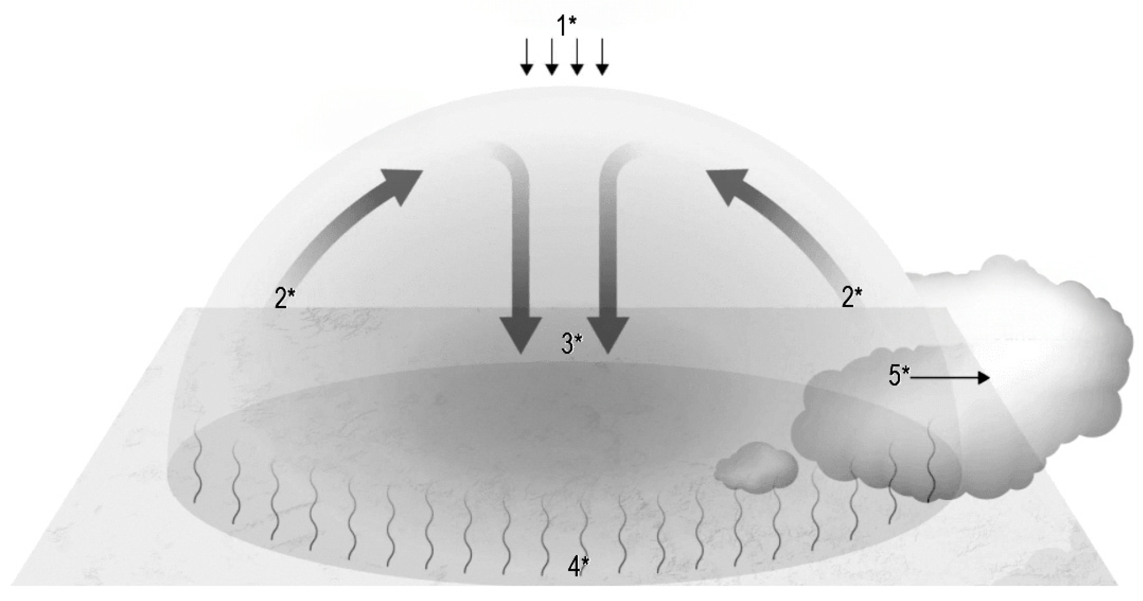
Figure 1. Schematic representation of a heat dome which involves high-pressure areas that trap and heat up the air below. This figure illustrates over a region that high pressure (1 *) in the atmosphere pushes warm air down toward the ground; hot air masses (2 *) expand vertically into the atmosphere as the air sinks (3 *) and it warms by compression; and the ground warms and loses its moisture, which makes it easier to heat even more (4 *). The dome of high pressure inhibits clouds and local rainfall and deflects away storms (5 *). These conditions lead to the onset of a flash drought, and consequences of the persistence of hydro-climatic anomalies over days or weeks can lead to substantial land degradation and desertification [4].
Atmosphere 15 00761 g001
Figure 2. Caatinga vegetation map. It comprises the following states in Brazil: Alagoas (AL), Bahia (BA), Ceará (CE), Minas Gerais (MG), Maranhão (MA), Paraíba (PB), Piauí (PI), Pernambuco (PE), Rio Grande do Norte (RN), and Sergipe (SE).
Atmosphere 15 00761 g002
Figure 3. An example of (a) the observed precipitation (P) and (b) satellite retrievals for surface soil moisture (SMOS-based SSM data) obtained in an agricultural area across the study area. The linear correlation between these two variables is indicated by the R2 = 0.70 from January 2016 to December 2020.
Atmosphere 15 00761 g003
Figure 4. As in Figure 3 (a) the observed precipitation but referring to (b) NDVI [dimensionless]. The NDVI was derived from the MSG-SEVIRI product. The dry spell occurred in 2012 and is highlighted with red bars.
Atmosphere 15 00761 g004
Figure 5. As in Figure 4 (a) the observed precipitation but referring to (b) the SPEI [dimensionless; base period January 2010–December 2020].
Atmosphere 15 00761 g005
Figure 6. Schematic overview of the individual steps of the deep learning processing for FD detection. The input-selected hydro-climatic variable (1 *) is taken by following a different sampling strategy for the training stages (2 *). A batch of selected variables (3 *) defines a sample received as input by the model, and a 2D convolutional encoder–decoder architecture provides probabilistic scores (4 *) for an FD as its output.
Atmosphere 15 00761 g006
Figure 7. Schematic overview of the proposed SCED for drought detection. The model receives as input a selected data variable and provides a probabilistic FD detection map for multiple timesteps as its output. Represented by color are the 2D convolution + 2D batch normalization + LeakyReLU activation, 2D (spatial) pooling, 2D (spatial) upsampling, and 2D out convolution. At the bottom of each 2D convolution + 2D batch normalization layer + LeakyReLU activation, the output spatial size in terms of (lat, lon) is indicated. Skip connections are placed between the input of an encoder block and the activation layer of the corresponding decoder block.
Atmosphere 15 00761 g007
Figure 8. Results of the analysis on the driving hydro-climatic data of temporal responses over the entirety of NEB during 2010–2016. (a) The squared wavelet coherence of the SPEI against the SSM, and (b) the lagged correlations between the SPEI and the variables involved (SSM, NDVI, and PET).
Atmosphere 15 00761 g008
Figure 9. (a) Time series of the five-day moving average of the daily SMOS-based SSM values over the entirety of NEB from 1 March to 28 December 2012. The dashed orange line and dashed red line represent the 40th and 20th percentiles for soil moisture, respectively. The blue dot represents non-FD (condition 1), and the green dot represents FD (condition 2). (b) The blue–orange vertical time series of anomaly values represents the period of precipitation (P) and potential evapotranspiration (PET) data from 2 May to 28 November 2012. The vertical dashed blue lines indicate the period between the FD conditions.
Atmosphere 15 00761 g009
Figure 10. Visual comparison of the performance of (a) the SMOS-based SMOS L3 SSM product and (b) the S-CED model trained with SSM data for the 2012 FD events identified from 1 March to 28 December 2012. The red color represents the higher scores of the model trained with the SSM. In contrast, green means lower values of the model. The Brazilian drylands boundary is displayed as the blue line (left side), and northeastern Brazil and its states in blue lines (right side).
Atmosphere 15 00761 g010
Figure 11. FD severity in SSP-8.5 identified in the growing season (February–May) from 2024 to 2050 within northeastern Brazil. Brazilian drylands boundary denoted by blue line.
Atmosphere 15 00761 g011
Table 1. Details of data sources.
Product/Data NameTime
Period
Temporal
Resolution
Spatial
Resolution
Data SourceAccessed on
P2010 to 2020Daily0.1°https://github.com/AlexandreCandidoXavier/BR-DWGD15 November 2023
PET2010 to 2020Daily0.1°
SMOS L3 SSM (asc)2010 to 2020Daily0.225°http://bec.icm.csic.es10 October 2023
SMOS L3 SSM (des)2010 to 2020Daily0.225°http://bec.icm.csic.es10 October 2023
NDVI2010 to 2020Daily3 kmhttps://lapismet.com.br/12 November 2023
Table 2. Thresholds used for flash drought classification.
Drought CategorySPEIProbability [%] 1SSM
Non-drought>1.00>77.50>25th
Near normal (FD1)0.99 to −0.9968.3020th–25th
Moderate dry (FD2)−1.00 to −1.499.2015th–20th
Severe dry (FD3)−1.50 to −1.994.4010th–15th
Extreme dry (FD4)<−2.002.30<10th
1 The cumulative probability of non-exceedance for each SPEI drought category.
Disclaimer/Publisher’s Note: The statements, opinions and data contained in all publications are solely those of the individual author(s) and contributor(s) and not of MDPI and/or the editor(s). MDPI and/or the editor(s) disclaim responsibility for any injury to people or property resulting from any ideas, methods, instructions or products referred to in the content.