A GPU-Implemented Lattice Boltzmann Model for Large Eddy Simulation of Turbulent Flows in and around Forest Shelterbelts

Abstract

Using porous wind barriers for the microclimate modification of agricultural lands, urban areas, and surrounding roads is a ubiquitous practice. This study establishes a new method for numerically modeling the turbulent flow in and around forest shelterbelts using an advanced multiple-relaxation-time lattice Boltzmann model (MRTLBM). A detailed description is presented for a large eddy simulation (LES) of turbulent winds by implementing barrier element drag force in the MRTLBM framework. The model results for a forest shelterbelt are compared with a field observational dataset. The study indicated that our implementation of drag force in MRTLBM is an accurate method for modeling turbulent flows in and around forest patches. Sensitivity analyses of turbulent flow related to the shelterbelt structure parameters and wind directions are also carried out. The analysis indicated that the optimal wind shelter effect in reducing the mean wind speed and turbulent kinetic energy is maximized using a narrow, medium porosity shelterbelt, with the wind direction perpendicular to the shelterbelt. These conclusions are in agreement with other observational and modeling studies. Finally, the computational time of a central processing unit (CPU) and graphics processing unit (GPU) was compared for a large domain with 25 million grids to demonstrate the MRTLBM advantage of LES in regards to computational speed with a mixed forest and building environment. The GPU is approximately 300 times faster than a CPU, and real-time simulation for this large domain is achieved using the Nvidia V100 GPU.

1. Introduction

Natural and human-grown forest patches are prevalent landscape components in urban and complex terrains, playing an important role regarding the microclimate near the ground’s surface. A forest canopy can affect wind, temperature, radiation sheltering, acoustic noise, and aesthetics in the atmospheric boundary layer. This study is focused on the effect of a forest shelterbelt on wind and the associated turbulent kinetic energy under a neutral atmospheric stability condition. The objective is to develop and validate a large eddy simulation (LES) model based on a multiple-relaxation-time lattice Boltzmann model (MRTLBM) for predicting the wind field and turbulence in and near the forest canopies.

The experimental and observational studies of forest wind barriers began early in the 20th century because forest shelterbelt usage in wind modification projects for agricultural and other purposes were common and effective. The wind shelter effect was summarized and analyzed from field observational results [1,2,3,4,5,6,7,8], most of which were focused on averaged steady mean wind speed because early anemometers were not able to reliably measure the turbulence. Some wind tunnel tests [9,10,11,12] were also carried out to simulate the wind barrier effect in different wind barrier arrangements over flat terrain. These observational studies and wind tunnel tests accumulated good knowledge and data for the validations of numerical models. Thom introduced the theoretical study and parameterization of the canopy drag force [13]. This was an important step due to the implementation of the porous canopy drag force as a body force term in Navier–Stokes equations (NSE). The numerical method was further developed to simulate turbulent flow in and above the forest canopies for time and spatial averaging using the governing NSE [14,15,16,17]. Two and/or three-dimensional NSE, based on numerical models using the Reynolds averaged simulation (RANS), were developed by many researchers [17,18,19,20,21,22]. The steady RANS is usually a time-averaged model, parameterizing turbulence in the same manner in all scales, using the concept of balance of turbulent kinetic energy (TKE) production and dissipation. These RANS simulations capture the mean wind and turbulence intensity of a turbulent flow reasonably well when compared with steady field and laboratory data but are not able to simulate the transient structure of turbulence. LES models [23,24] resolve the turbulent eddies which are larger than the grid-scale and represent a major step forward in turbulence modeling due to their capability to simulate transient structures under unsteady flows. The LES model method parameterizes small sub-grid scale turbulence and explicitly resolves turbulent eddies that have greater length scales than those of the computation grid. However, LES models usually use a large number of computation grids and require more computational resources when compared with the steady RANS model. In recent years, NSE-based LES models were employed by several researchers [25,26,27,28,29] for turbulent flows in and around wind barriers.

The lattice Boltzmann method (LBM) for modeling the fluid dynamic problem was initiated in the early 1990s [30,31,32]. Unlike traditional computational fluid dynamics methods that numerically solve continuum-based macroscopic flow velocity variables ($\rho$, u, v, w) in NSE, the LBM is a kinetic, particle-based mesoscopic method for solving the Boltzmann equation in which the particle probability distribution function (PDF) is the control variable. The LBM solves the particle PDF via collision and streaming for energy and momentum propagation in fluid at each lattice node. The macroscopic fluid variables (e.g., density $\left[\rho \right]$ and velocity [u_i]) are derived from the zero, first-order statistical moments of the PDF. The LBM has several advantages, including the simplicity of its code development, its easier implementation of complex boundary conditions, and its intrinsic parallelism for massively parallel computing. In NSE-based RANS or LES models, the nonlinearity advection terms are usually computed by several neighboring grid points, depending on the order of accuracy. This makes parallel processing more difficult, and the pressure equation in the incompressible flow in NSE-solvers is a Poisson equation that takes many iterations to solve for each time step. With the LBM, the nonlinear processes are handled in an individual computation grid, making parallel processing more efficient. Furthermore, the dynamic pressure field is derived from a simple diagnostic relationship using the density fluctuation in LBM. Details about the history, fundamental theory, and methods of LBM are available in the literature [30,31,32]. The LBM has undergone significant developments in the last three decades. An LBM based on the Bhatnagar–Gross–Krook collision [33], called LBGK, was the first to be developed and subsequently, the most popular method implemented at the beginning of the LBM development era [34,35]. Using LBGK, the collision process is performed with a single-relaxation time parameter. While LBGK is an accurate method for solving low-Reynolds number laminar flow problems, it is not numerically stable and is inaccurate for simulating a high-Reynolds number turbulent flow. More recently, several varieties of LBM methods have been developed to remedy this critical problem [36,37,38,39,40,41].

We used the multiple-relaxation-time Lattice Boltzmann method (MRTLBM) developed by d’Humières et al. [39,40]. In MRTLBM, the fluid particle collision processes are performed in a moment space, and the PDF moments are relaxed at different rates to achieve better accuracy and numerical stability for turbulent flow. This method has been demonstrated to be superior for simulating turbulent flows over single-relaxation LBGK, in which collisions are represented with a single-relaxation rate [40,42]. In a recent analysis of Chai and Shi [43], they presented a new MRT-LBM with a block-lower triangular-relaxation matrix obtained from the discrete velocity Boltzmann equation through some proper discretization of time and space. Since the Reynolds number in atmospheric turbulent flows is usually large, it is critically important to use the MRTLBM or other improved LBMs for atmospheric boundary layer flow modeling. Other types of advanced LBMs have been developed for simulating turbulent flows in an infinite homogenous forest canopy over flat terrain [44,45]. To our knowledge, this is the first effort to develop and validate the capability of the MRTLBM in the simulation of a forest shelterbelt. We have developed an atmospheric boundary layer environment model using the MRTLBM, using this model to simulate the laboratory case of stratified turbulent flows over a ridge terrain [46] and around and overhead urban buildings [47,48]. The results show that this is an accurate and fast model for urban turbulent flow modeling using a graphical processing unit (GPU). In this continuation of our research, we extend the model’s capability for the flow in and around porous forest canopies.

2. The Numerical Model and Vegetation Drag Force Implementation

2.1. The ABLE-LBM Model

The numerical model used in this study is a newly developed microscale atmospheric boundary layer model that is called the atmospheric boundary layer environment–lattice Boltzmann model (ABLE-LBM). It is a four-dimensional prognostic LES model based on an MRTLBM [39,40,41,46,47,48]. It is used for fine-scale (temporal: seconds; spatial: meter to tens of meters) atmospheric boundary turbulent flows and the associated transport and dispersion of temperature, moisture, and other scalars (aerosol, smoke).

Instead of numerically solving the NSE, the LBM is a mesoscopic method that tracks the PDF of air parcel (or fictitious particle) motion and collision in certain prescribed sample directions that connect to neighboring computation grids. It can start with the evolution equation of the MRTLBE coupled with the forcing term [39,40,41,46,47,48]

$$\mathit{f}\left(\overrightarrow{x}+{\mathit{c}}_{\mathit{\alpha }}dt,t+dt\right)-\mathit{f}\left(\overrightarrow{x},t\right)={\mathrm{\Omega }}_{\mathit{\alpha }}+\mathit{F}dt$$

(1)

where $\mathit{f}$($\overrightarrow{x,}$ t) is a single particle PDF in phase space; ${\Omega }_{\mathit{\alpha }}$ is the collision operator; $\mathit{c}$ is the particle velocity; $\mathit{F}$ is the external forces (including buoyancy and drag forces). The collision is the process of relaxing to the Maxwell–Boltzmann equilibrium distribution, ${\mathit{f}}^{eq}$. In the LBM of the 3D flow problem, there are different lattice models—D3Q15, D3Q19, D3Q27—where Q denotes the number of lattice directions. In the ABLE-LBM, we chose 19 lattice directions for the parcel collision and streaming. The Taylor expansion of the ${\mathit{f}}^{eq}$ can be written in the following form by neglecting the third order terms:

$${\mathit{f}}^{eq}=\rho {\mathit{w}}_{\mathit{\alpha }}\left[1+\frac{{\mathit{c}}_{\mathit{\alpha }}{u}_i}{c_s^2}+\frac{{\left({\mathit{c}}_{\mathit{a}} u_i\right)}^2}{2c_s^4}-\frac{u_i^2}{2c_s^2}\right],$$

(2)

where $u_i$ is the fluid macroscopic velocity; $c_s=c/\sqrt{3}$ is the lattice sound speed; and ${\mathit{c}}_{\mathit{\alpha }}$ is the lattice speed in 19 directions, expressed in our model as:

$${\mathit{c}}_{\mathit{\alpha }}=\left\{\begin{array}{c}\left(0,0,0\right) \alpha =0\\ \left(\pm 1, 0, 0\right)\left(0,\pm 1, 0\right)\left(0, 0,\pm 1\right) \alpha =1,\dots , 6\\ \left(\pm 1,\pm 1, 0\right)\left(\pm 1, 0,\pm 1\right)\left(0,\pm 1,\pm 1\right) \alpha =7,\dots , 18\end{array}\right..$$

(3)

The ${\mathit{w}}_{\mathit{\alpha }}$ is the weighting factor in the lattice directions:

$${\mathit{w}}_{\mathit{\alpha }}=\left\{\begin{array}{cc}\frac{1}{3},& \alpha =0\\ \frac{1}{18},& \alpha =1,\dots , 6\\ \frac{1}{36},& \alpha =7,\dots , 18\end{array}\right..$$

(4)

In the LBGK, only single-relaxation time is used to characterize the collision effects. It is unrealistic to represent the collision to equilibrium in the same relaxation for all the physical modes (e.g., momentum and energy) [41]. In the MRTLBM, a collision matrix with different eigenvalues or multiple-relaxation times are used for different physical modes. The MRTLBM equation of the Boltzmann Equation (1) with α discrete particle velocities can be written in the following vector form with multiple-relaxation time [40,41,42]:

$$\mathit{f}\left(\overrightarrow{x}+{\mathit{c}}_{\mathit{\alpha }}dt,t+dt\right)-\mathit{f}\left(\overrightarrow{x},t\right)={-M}^{-1}S\left[\mathit{m}\left(\overrightarrow{x},t\right)-{\mathit{m}}^{\mathit{e}\mathit{q}}\left(\overrightarrow{x},t\right)\right]+M^{-1}\widehat{\mathit{F}}dt,$$

(5)

where $\overrightarrow{x}$ and t are space vector and time, respectively, and boldface denotes column vectors with α lattice directions. We used a D3Q19 lattice model, which has 19 lattice directions (α = 0, …, 18). The PDF $\mathit{f}$, for example, is written in the following column vector:

$$\mathit{f}\left(\overrightarrow{x},t\right)\equiv {\left(f_0\left(\overrightarrow{x},t\right),\hspace{1em}\hspace{1em}{f}_1\left(\overrightarrow{x},t\right),\hspace{1em}\dots ,f_{18}\left(\overrightarrow{x},t\right)\right)}^T.$$

(6)

The $\widehat{\mathit{F}}$ is the moment of the forcing term in moment space [31]; $\widehat{\mathit{F}}=\left[\mathit{I}-S/2\right]M{\mathit{F}}_{\mathit{\alpha }},$ where ${\mathit{F}}_{\mathit{\alpha }}$ is the body force vector; S is the diagonal relaxation matrix. The column vectors m and m^eq are the velocity moment vector and its equilibrium vector, respectively; M is a 19 × 19 matrix, which linearly maps the velocity space to the velocity moment space [40], $\mathit{m}=M\mathit{f}, \mathit{f}=M^{-1}\mathit{m}$. The moment vector components can be interpreted as the hydrodynamic quantities and their fluxes. The moment vector is arranged in the following order, with each component related to a physical property of the fluid:

$${\mathit{m}=(\rho \prime ,e,\epsilon ,j_x,q_x,j_y,q_y,j_z,q_z,{3p}_{xx},{3\pi }_{xx},p_{ww},{\pi }_{ww},p_{xy},p_{yz},p_{xz},m_x,m_y,m_z)}^T,$$

(7)

where $\rho \prime$ is the density fluctuation; e is related to energy; $\epsilon$ is related to energy squared; j_x, j_y, and j_z are the components of flow momentum; (j_x, j_y, j_z) = ${\rho }_0\overrightarrow{u}$, q_x, q_y, q_z are the third order moments corresponding to energy fluxes in x, y, and z directions, respectively; p_xy, p_yz, and p_zx are related to the components of the symmetric and traceless strain-rate tensor; ${\pi }_{xx} \mathrm{and}{ \pi }_{ww}$ are fourth order moments; and $m_x,m_y,{\mathrm{and} m}_z$ are the third order moments. The orthogonal transformation matrix M is derived using the Gram–Schmidt orthogonalization procedure [40]. Since M is an orthogonal matrix, its inverse M⁻¹ can be easily determined by multiplying it by its transpose. There are four conserved quantities in this MRTLBM; these are the density $\rho \prime$ and three components of momentum j_x, j_y, and j_z. By using the following decomposition of density, the compressibility effect of the model and round-off error are reduced, as follows:

$$\rho ={\rho }_0+{\rho }^{\prime },{\rho }_0=1.$$

(8)

The equilibrium function vector m^eq for the other non-conserved moments are given as follows [39]:

$$\begin{array}{c}{m}_1^{eq}=-11{\rho }^{\prime }+\frac{19}{{\rho }_0}\left(j_x^2+j_x^2+j_x^2\right),{{ m}_2^{eq}=\omega }_{\epsilon }{\rho }^{\prime }+\frac{{\omega }_{ej}}{{\rho }_0},m_{4,6,8}^{eq}=\frac{{\omega }_{ej}}{{\rho }_0},\\ m_9^{eq}=\frac{1}{{\rho }_0}\left(2j_x^2-j_y^2-j_z^2\right),{m_{10}^{eq}=\omega }_{xx}{m}_9^{eq},{{m_{11}^{eq}=\frac{1}{{\rho }_0}\left(j_x^2-j_z^2\right),m}_{12}^{eq}=\omega }_{xx}{m}_{11 }^{eq},\\ m_{13}^{eq}=\frac{1}{{\rho }_0}{j}_x{j}_{y,}{m}_{14}^{eq}=\frac{1}{{\rho }_0}{j}_y{j}_{z,}{m}_{15}^{eq}=\frac{1}{{\rho }_0}{j}_x{j}_{z,}{m}_{16}^{eq}=m_{17}^{eq}=m_{18}^{eq}=0.\end{array}$$

(9)

The parameters in Equation (9) are chosen to optimize the linear stability of the MRTLBM ${\omega }_{\epsilon }={\omega }_{xx}=0 \mathrm{a}\mathrm{n}\mathrm{d} {\omega }_{\epsilon j}=-\frac{475}{63}$. With the equilibrium moments above, the speed of sound c_s in the unit of lattice speed is $c\equiv \frac{dx}{dt}=1$.

The diagonal relaxation matrix S for the collision process in the moment space is

$$S=diag\left(0,s_{1,}{s}_{2,}0,s_{4,}0,s_{4,}0,s_{4,}{s}_{9,}{s}_{10,}{s}_{9,}{s}_{10,}{s}_{13,}{s}_{13,}{s}_{13,}{s}_{16,}{s}_{16,}{s}_{16}\right),$$

(10)

where the relaxation rates of the non-conserved moments are in the range of (0, 2) and are specifically related to the shear viscosity ($\nu$) and bulk viscosity (ζ) as

$$s_1=2/(9\zeta +1) \mathrm{and} s_9=s_{13}=2/(6\nu +1).$$

(11)

In this simulation, we use the following relaxation parameters for optimized stability [39,40]:

$$s_1=1.19,{ s}_2=s_{10}=1.4,s_4=1.2,s_{16}=1.98.$$

(12)

All the model parameters and their physical representations, such as the relaxation coefficients matrix S, moment vector (m), equilibrium moment vector (m^eq), and the transformation matrix (M) are described in the work of d’Humières et al. and Lallemand and Luo [40,41]. More detailed descriptions of the ABLE-LBM and its associated MRTLBM are available in the work of Wang et al. [46,47,48].

2.2. Modeling of Porous Element Drag Force in LBM System

Thom [13] reported that under the assumption of a high-Reynolds-number turbulent flow, the skin friction part of drag force is small and may be neglected. The vegetation drag force is mainly due to the pressure from drag, and its components in a Cartesian coordinate can be computed from a parameterized formula:

$$F_i=-{\frac{1}{2}\rho C}_{d}AU\left|u_i\right|, i=1,2,3$$

(13)

where $C_d$ is the nondimensional drag coefficient; A is the canopy vegetation element density; U is the total wind speed; and u_i respresents the velocity components in three Cartesian directions. It is important to note that the $C_d$ here is an averaged value and is often derived from the laboratory wind tunnel data. $C_d$ is a dynamic coefficient and is related to many factors, such as the shape and arrangement of canopy elements, as well as the Reynolds number. The magnitude of $C_d$ for a shelterbelt has a wide range of variation in the literature [5,7,9,21,28]; it is quite different for the infinite and homogenous vegetation canopies in other canopy models. In this study, we use $C_d=1.6$, which is derived from a wind tunnel test specifically employed for the observation of shelterbelt flow [49]. In the shelterbelt case, which is usually thin in width, the greatest drag force or momentum sink is due to the canopy, causing dynamic pressure difference at the windward and lee sides of the shelterbelt. In the modeling of thin artificial wind barriers, it is customary in shelterbelt modeling to use a resistance coefficient or pressure-loss coefficient k_r, in which the resistance coefficient is related to the drag coefficient and vegetation density in the following equation [17,21]:

$$k_r={\int }_{-W_{sb}}^0{C}_d A dx,$$

(14)

where $W_{sb}$ is the shelterbelt width. This equation will be useful for comparing our results with observational and other modeling results. Since the LBM lattice has 19 directions in ABLE-LBM, the drag force is then distributed in each lattice directions, according to Ref. [50], as follows:

$${\mathit{F}}_{\mathit{\alpha }}={\mathit{w}}_{\mathit{\alpha }}\left(\frac{{\mathit{c}}_{\mathit{\alpha },i-}{u}_i}{c_s^2}+\frac{{\mathit{c}}_{\mathit{a},j}{u}_j}{c_s^4}{\mathit{c}}_{\mathit{\alpha },i}\right)F_i,$$

(15)

where $u_i$ are the macroscopic wind velocity vector components computed from the previous step. The ${\mathit{F}}_{\mathit{\alpha }}$ is used in Equation (15) for the drag force effect in each lattice direction. The macroscopic air density and velocity are computed as follows:

$$\rho ={\sum }_{\alpha =0}^{18}{\mathit{f}}_a, u_i={\sum }_{\alpha =0}^{18}{\mathit{c}}_{\alpha ,i}{\mathit{f}}_{\alpha }+\frac{dt}{2}{F}_{i }, p=c_s^2\rho ,$$

(16)

where p is the dynamic pressure. The pressure is computed diagnostically from the density, which is another advantage of the LBM over the NSE-based model.

2.3. Sub-Grid Turbulence Parameterization

The Lily–Smagorinsky turbulence model [23,24] is used for the sub-grid turbulence in this research. It uses the eddy viscosity that is related to the local strain-rate tensor for Reynolds stress parameterization, analogy to the molecular momentum diffusion determined by molecular viscosity. The equation for total momentum diffusion at sub-grid scales is determined by a total effective viscosity (${\nu }_{total}$) that includes molecular viscosity ($\nu$) and turbulent viscosity (${\nu }_t$):

$${\nu }_{total}=\nu +{\nu }_t={(C∆)}^2\overline{S},$$

(17)

where C is a constant, which is taken as 0.2; Δ is the filter size, taken as the grid size; and $\overline{S }$ is the magnitude of the filtered strain-rate tensor:

$$S=\sqrt{2S_{ij}{S}_{ij}},$$

(18)

where $S_{ij}=\frac{1}{2}\left(\frac{\mathsf{\partial }{u}_i}{\mathsf{\partial }{x}_j}+\frac{\mathsf{\partial }{u}_j}{\mathsf{\partial }{x}_i} \right), \mathrm{a}\mathrm{n}\mathrm{d}$ $u_i$ represents the macroscopic wind vector components computed from the previous step. The strain-rate tensor components can be computed directly from the nonequilibrium moments in the LBM [51]. The strain-rate tensor, $S_{ij}$, is computed using the equations from:

$$\begin{array}{c}{S}_{xx}=-\frac{1}{38{\rho }_{0}dt}\left(s_1{m}_1+19s_9{m}_9\right),\hfill \\ S_{yy,zz}=-\frac{1}{76{\rho }_{0}dt}\left(2s_1{m}_1-19s_9(m_9\mp 3m_{11}\right),\hfill \\ S_{xy,yz,zx}=-\frac{3s_9}{2{\rho }_{0}dt}{m}_{13,14,15}.\hfill \end{array}$$

(19)

Here, ${\rho }_0$ is the background fluid density, and $s_{i, }\mathrm{and} m_i$ are the multiple-relaxation coefficients and moments components, respectively. For a more detailed description of the sub-grid turbulence modeling, see Wang et al. and Yu et al. [46,51].

There is an effect of the forcing term on computing the strain-rate tensor [52]. Since this implementation of MRTLBM includes a drag force term of vegetation elements, a small error in the strain-rate term could be caused by using Equation (19). Our flow regime is highly turbulent compared with the results of previous analyses [52]. It is worthwhile to investigate this effect in future studies.

3. Results and Discussion

3.1. Simulation of a Forest Shelterbelt

The first validation case uses the data from a field observation by Kurotani et al. [6] in Izumo, Japan. In their study, an inflow reference tower and five towers on the lee side of the shelterbelt were installed for mean wind and turbulent kinetic energy profiles using 3D sonic anemometers over a flat terrain. Figure 1 shows the observational setups with a reference tower mounted at three levels for the inflow conditions at x = −5 H. The other dimensions of the shelterbelt were 74 m in length and 2 m in width. There is a trunk area in the shelterbelt without leaf elements, ranging from the ground level to 1.2 m high. The five profiles (P₁–P₅) were located at distances of 1 H (7 m), 2 H (14 m), 3 H (21 m), 4 H (28 m), and 5 H (35 m), respectively, on the lee side of the shelterbelt. Four levels of observation at heights of 1.5 m, 3.0 m, 4.5 m, and 6.0 m were carried out at each observational profile (P₁–P₅).

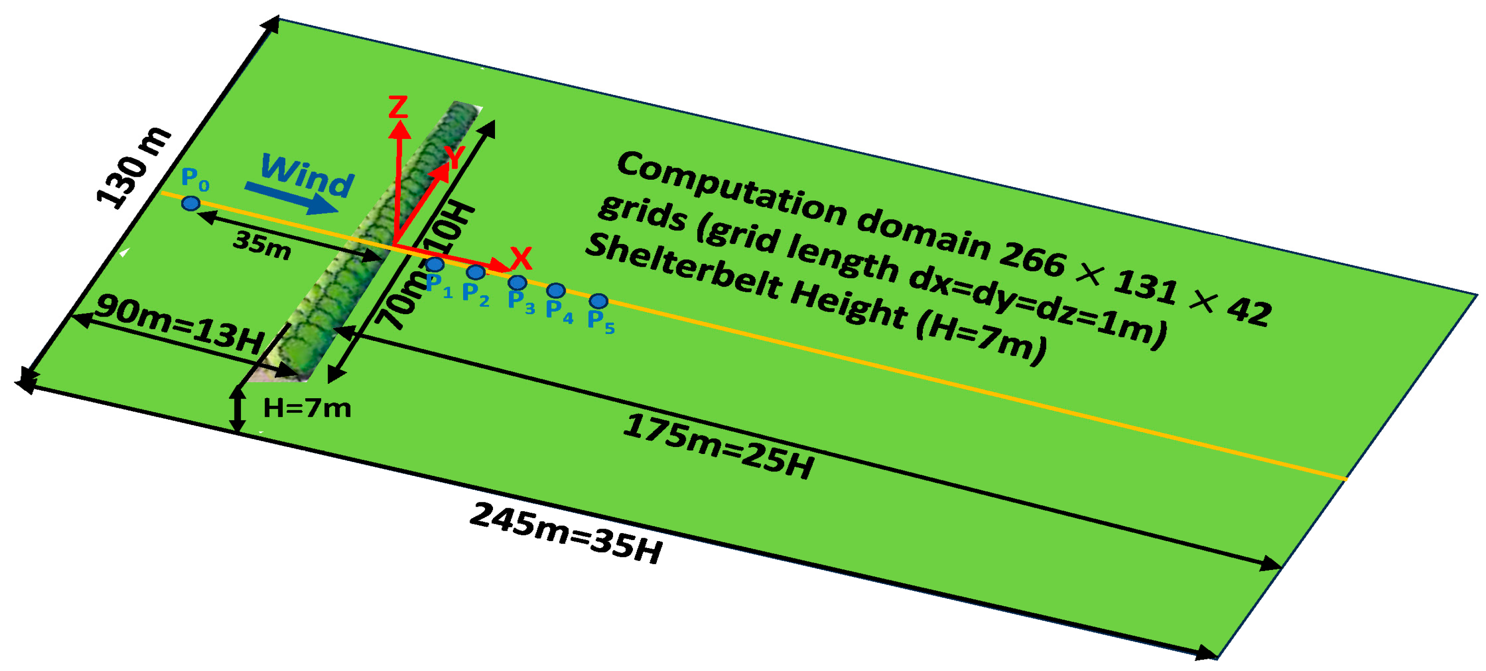
The setup of the domain simulation is shown in Figure 2. The domain is a box with a length of 35 H, a width of 18.6 H, and a height of 6 H over flat terrain, where H = 7 m and is the height of the shelterbelt. The grid lengths are 1 m in the x, y, z directions, resulting in grid numbers of 265 × 131 × 42. The forest shelterbelt with dimensions of 2 m in width, 7 m in height, and 70 m (10 H) in length was set up at the x = 90 m in the domain. The observed wind profiles (Figure 1) are placed at the y = 0 m, which is the vertical xz symmetry plane in Figure 2. In this simulation, the grid lengths were Δx = Δy = Δz = 1 m. The vegetation element density A = 1.18 m⁻¹ was used in this simulation, according to methods provided in the literature [28,29,48].

The data selected for the model validation was obtained from 12:30 to 14:50 on 20 December 2000 [6]. The atmospheric stratification condition was neutral, and the wind was basically perpendicular to the shelterbelt, with small deviation from −10° to 0° from the perpendicular line. The inflow mean wind speed was quite stationary at approximately 5.5 m/s at the height of 5.36 m. The LES simulation requires not only the observed mean wind profile of the approaching wind, but also the turbulent fluctuations for the inflow boundary condition. We used a simple synthetic algorithm [48] for the turbulence part of the inflow that agreed with the observed profile. The inflow boundary profiles are shown in Figure 3. The left panel shows the inflow profiles of the observed mean wind speed and turbulent kinetic energy (TKE) at the reference tower P₀. The computed mean wind speed and TKE at the same point (P₀) are also plotted in the right panel of Figure 3 to assure that the inflow boundary conditions agree with the observations. The mean wind profile at the reference point also agreed with the neutral logrithmic wind profile, $u=\left(u_{\ast }/k\right)ln\left[(z+z_0)/z_0\right]$, where $u_{\ast }$ = 0.34 m/s is the friction wind speed; k = 0.41 is the Von Karman constant; and $z_{0 }$= 0.01 m is the roughness length. The surface boundry condition was set up using the logarithmic profile for the first model layer height, since the large eddy scale is smaller than the model level. An open outflow boundary condition was used at x = 175 m (25 H). A free-slip boundary condition was set for the top boundary at z = 42 m (6 H), and cyclic boundary conditions were set for the lateral boundary condition to avoid the limitation of lateral boundaries.

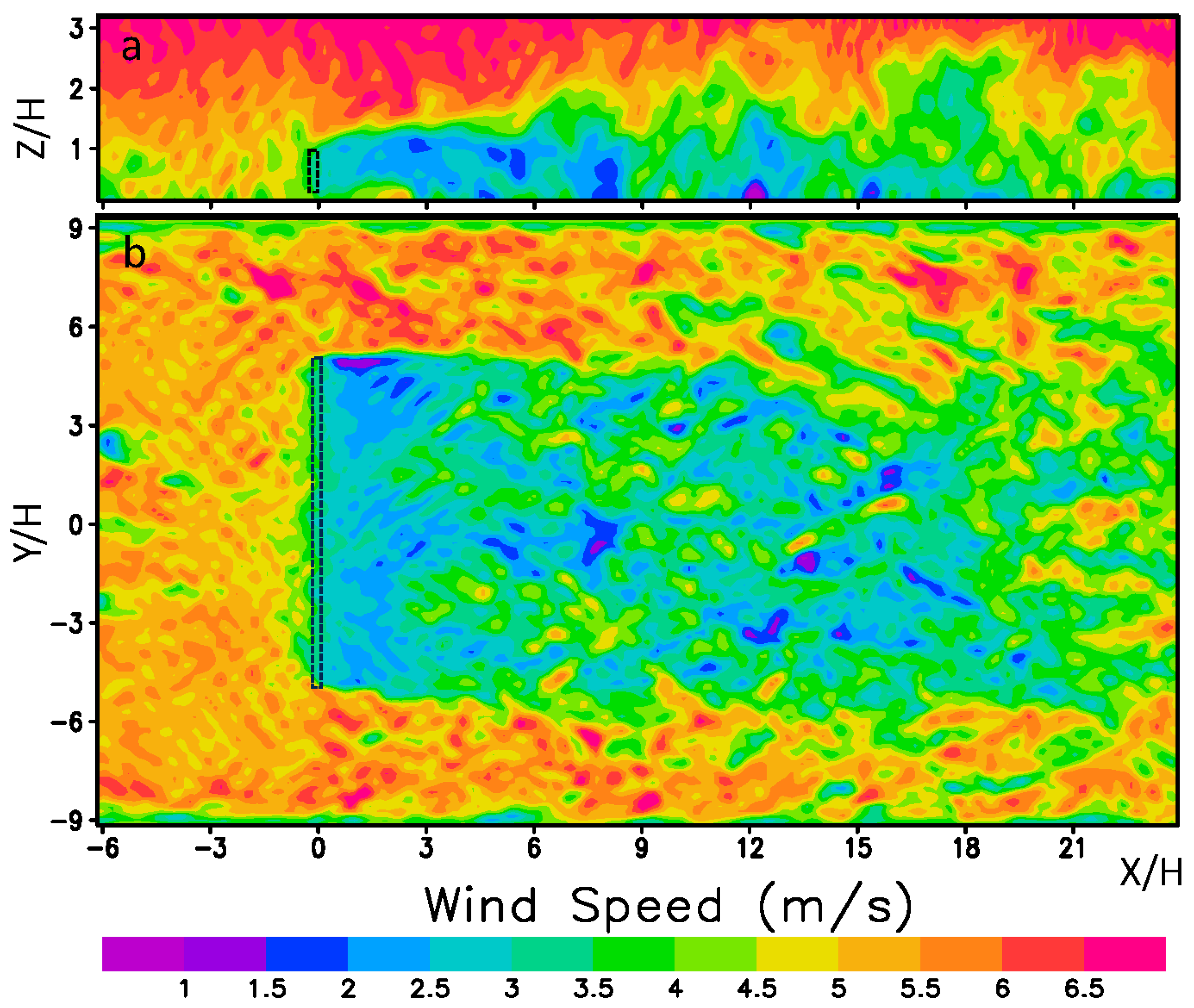
Figure 4 displays an instantaneous wind field of vertical (a) and horizontal (b) cross section results at t = 800 s of the model simulation results, just to show the characteristics of a turbulent wind field. For a clearer view of the turbulent variations, note that the scale of the vertical axis of (a) is not the same as the horizontal axis. The LES model resolves the larger scale turbulent eddies which are greater than the grid length, while the turbulent eddies smaller than the grid length are modeled using the Lily––Smagorinsky parameterization [23,24]. The vertical cross section shows a typical shelterbelt zone, as illustrated in Judd et al. [9] from a wind tunnel study; a bleed flow (x = 0–2 H, Z = 0–1 H), where the turblent fluctuations are dissipated by the canopy; a displacement zone (x = 0–8 H, z > 1 H), where wind speed is greater than the upstream wind; a quiet zone (x = 2–8 H, z < 1 H), where wind speed is greatly reduced; and a recovery zone (x = 8–20 H, z = 0–2 H), where the wind gradually returns to the upstream state. The recovery zone displayed more wind variations because the upper-level higher energy flow penetrated toward the ground level via Helmoholtz instability. Generally, the turbulent eddies are elongated in the mean flowing (x) direction compared with the vertical direction. The lee wake area is still evident at x = 21 H, which qualitatively agrees with many previous studies [5,9,19,21,25,28]. The leeside wakes are up to 2–3 H vertically at a distance of 9–18 H in the x direction.

By taking the time average of the model output results at each grid point, the LES model results can be compared with the observational data [6], which showed the time average for a period of stationary turbulent flow. The time average for each component separates the wind component into average and turbulent fluctuation parts:

$$u_i={\overline{u}}_i+u_i^{\prime }, i=1,2,3$$

(20)

where ${\overline{u}}_i=\frac{1}{T}{\int }_0^T{u}_{i }dt$, and TKE is computed as:

$$TKE=\frac{1}{2}\left({\sigma }_u^2+{\sigma }_v^2+{\sigma }_w^2\right),$$

(21)

where ${\sigma }_i^2$ represents the variations in the three velocity components.

Figure 5 and Figure 6 are the plots of the comparisons of the average mean wind profiles and TKEs, respectively, at the observational points denoted in Figure 1. The simulation requires some time for the inflow information to proceed through the entire simulation domain to reach a quasi-stationary flow state. To avoid the results in the un-stationary spin up time, the time average of the LES simulation was taken from t = 500 to t = 1500 s. The averaged wind vertical profiles at x = 1 H, 2 H, 3 H, 4 H, and 5 H compare reasonably well with those of the observation. The fact that the shelterbelt at the bottom has a 1.2 m open trunk space is reflected in the observational data simulation results in this region of the lee side flow. These simulation results are consistent with those of other simulations [28,29].

The grid size independence of the numerical method model was also checked using the refinement. In this case, the grid refinement is also a good way to show that the grid size is adequate for the flow problem to be modeled. In some very complex situations, the scales of large turbulent eddies are so different that local refinements may be needed. In a refined-grid simulation, the grid size was set to be Δx = Δy = Δz = 0.5 m, with the number of grid points of 530 × 262 × 84 for the same computational domain. The simulation results are shown with green lines for mean wind in Figure 5 and for TKE Figure 6. The results of the refined-grid simulation are very close to the results obtained for the original grid size of 1 m. This sensitivity indicated that a 1 m uniform grid was adequate to resolve the turbulent flow field for this simulation problem.

Figure 7 displays an averaged dynamic pressure field ($p^{\prime }=(p-p_0)/{\rho }_0)$ computed from the LES model at the center vertical cross section at y = 65 m. The plot shows that there is a larger, abrupt pressure gradient at the leading edge of the shelterbelt, with positive pressure at the windward side leading edge and negative pressure at the lee side of the leading edge of the shelterbelt. The results agree well with those of other studies [9,21]. The pressure field is closely co-related with the wind field and shows a major driven force for the mean wind reduction of the shelterbelt.

3.2. The Sensitivity of Turbulent Flow Field to Shelterbelt Structures and Wind Directions

In the preceding model validation, a specific shelterbelt structure of the field observation [6] was considered, and the wind direction was perpendicular to the long axis of the shelterbelt. In many other shelterbelt application designs, the structures of the shelterbelt (including width, height, and vegetation element density) are more likely to be different from those in the previously mentioned experiment site. Wind directions are probably not perpendicular to the shelterbelt long axis. These factors deserve a sensitivity analysis for the application point of view. In the following sensitivity analysis, we used the same inflow mean and turbulent profiles for simplicity, and the shelterbelt was uniform in terms of vegetation element distribution from the ground up (no gap was near the ground).

3.2.1. Vegetation Element Density

The vegetation element density of the shelterbelt is one of the important structure parameters for determining the flow fields of the shelter effects. Figure 8 shows the sensitivity of the mean wind speed and TKE with respect of different shelterbelt vegetation element densities. In this test, all the inflow winds originate from the west and blow perpendicular to the shelterbelts. The shelterbelts were kept in the same geometric dimension, although the vegetation element densities varied from small to large. The average lee side wind speed at ½ H were reduced by 30% for A = 0.19 m⁻¹ (Figure 8a), while the speed reduction was approximately 60% for A = 2.25 m⁻¹ (Figure 8d). The sections exhibiting the greatest wind reduction are located at a distance of 3–15 H away on the lee side of the shelterbelt. The sheltered distances for the portions exhibiting the largest wind reductions in the x direction were decreased as the vegetation element density increased. The TKE distribution was highly related to vegetation element density. The shelterbelt showed better TKE reduction in low vegetation density shelterbelts (Figure 8e,f). While the TKE decreased in x direction from 0–6 H in all cases (Figure 8e–h), the TKE increased and extended higher up in the z direction as the vegetation element density increased. This TKE increase indicated that the flow on the lee side was more turbulent as the vegetation element density increased. The shelter effects involve not only the mean speed reductions, but also the turbulent intensity alteration due to the shelterbelt, which has significant implications for some specific applications.

3.2.2. The Width of the Shelterbelt

Given the same vegetation element density distribution, the shelterbelt’s width has a large influence on the shelter effects on the lee side [21,27,28]. Figure 9 shows the averaged wind vertical cross sections at y = 65 m. The model simulation using a 2 m wide shelterbelt (Figure 9a) produced an approximately 30–40% reduction in mean wind speed, while the shelterbelt with a 15 m width (Figure 9c) showed an approximately 80–90% reduction in the mean wind speed. The TKE also showed dramatic differences; while the 0–3 H on the lee side displayed a reduction of TKE for both narrow and wide shelterbelts, the TKE from x = 3–24 H exhibited greater TKE values for the wide shelterbelt, especially in the upper level of the domain. These tests indicate that wider shelterbelts produce a greater number of large turbulent eddies on the lee side, due to more pressure being drag-produced in the wider shelterbelt. Furthermore, when the shelterbelt is wide enough, a stationary boundary layer could develop above the canopy—a different turbulent regime when compared with the flow around shelterbelts. The results have important implications in regards to shelterbelt designs for specific applications.

3.2.3. The Wind Directions and Shelter Effects

The effectiveness of the shelterbelt is related to the angles of the incoming wind direction relative to the shelterbelt long axis direction, as documented in earlier studies [8,18,21,28]. In this sensitivity study, the LES model was used to test different wind angles with respect to the effectiveness of the shelterbelts. Figure 10 shows the shelterbelt effectiveness in reducing the wind speed and in altering the TKE in three approaching wind angles, with respect to the shelterbelts. All these runs used the same shelterbelt dimensions and vegetation element densities. Figure 10a shows an instantaneous wind (t = 1000 s) incoming perpendicular to the shelterbelt; Figure 10b shows an instantaneous wind occurring simultaneously to wind coming in at 45° with respect to the shelterbelt; and Figure 10c is an instantaneous wind occurring simultaneously to an incoming wind of 60° with respect to the shelterbelt. The sheltered areas are larger for small angles of incoming wind. The 60° incoming wind exhibited less than a quarter of the sheltered area when compared with the perpendicular wind. However, the wind speeds exhibited a larger reduction in the affected areas in the cases of non-perpendicular wind (Figure 10b,c). This is due to the longer air parcel travel length inside the shelterbelt for the non-perpendicular cases. The bottom panel plots (Figure 10d–f) show the average TKE corresponding to the cases (Figure 10a–c), respectively.

The smaller wind angles with respect to the shelterbelt showed large areas of TKE reduction in the shelterbelts. The larger TKE at the south and north edges of the shelterbelts all displayed larger TKE in all three runs because these areas represent the interfaces of the shelterbelt’s affected and nonaffected areas where the turbulent motions produced intensive turbulent activities, especially in regards to the nonstationary turbulent eddies due to the shear production.

3.3. GPU Implementation of the ABLE-LBM and Model Execution Speed

One of main advantages of the LBM as compared to the traditional CFD method is that the LBM is more suitable to the massive parallelization of the GPU architecture. Modern GPUs have thousands of computer cores and thus can run thousands of threads simultaneously, especially for memory intensive problems. The LBM algorithm is memory-intensive due to 19 direction of lattice directions. The data locality in the LBM is satisfied, and time-stepping is explicit. Each computation grid cell in the domain is assigned to a GPU thread. The simulation is written in Compute Unified Device Architecture (CUDA) (Nvidia, Santa Clara, CA, USA). In our implementation, the 3D computation grids are mapped to 1D memory. In GPUs, the threads are executed in lockstep sets called warps. The threads within each warp need to load memory together to use the hardware effectively; this is called memory coalescing. In the implementation, we manage this by ensuring that threads within a warp are accessing consecutive global memory as often as possible. For instance, when calculating the moment vector in Equation (5), we load all 19 lattice velocities per grid cell. We organize the velocities so all the values for each specific direction are consecutive in the memory. This way, as the threads of a warp access the same direction across consecutive grid cells, and these memory accesses can be coalesced.

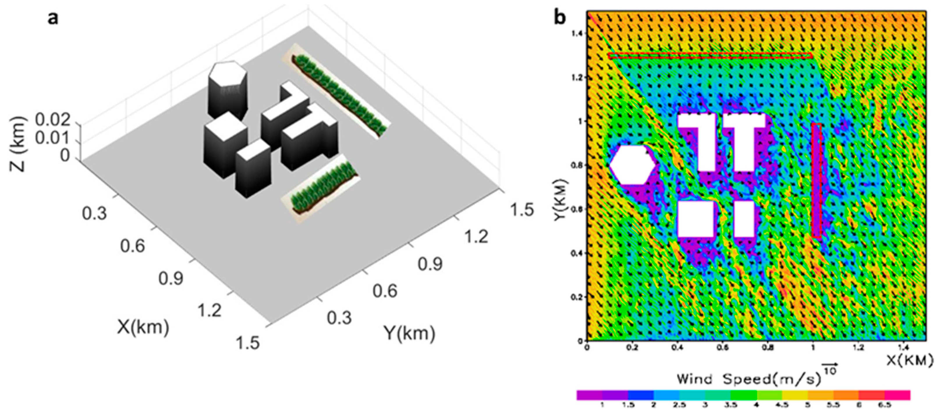
A large model domain with a grid number with 25,351,101 grid points (501 × 501 × 101) was chosen to test the ABLE-LBM’s computation efficiency in regards to GPU implementation. There were several large buildings and two shelterbelts in the domain. Figure 11 shows the 3D picture of the domain and the instantaneous (1000 s) turbulent wind field within the ABLE-LBM LES. The turbulent structures around buildings and shelterbelts are shown. The model resolution of the domain is 3 m (Δx = Δy = Δz = 3 m), covering an area of 1.5 × 1.5 km.

Table 1. Model execution time using a CPU and GPUs for a 1 h flow time in a domain (see Figure 11) with 5,352,101 (501 × 501 × 101) grids.

	Intel X5650 CPU (Hours)	Nvidia P100 GPU (Hours)	Nvidia V100 GPU (Hours)
	236.82	1.84	0.78
CPU/GPU time ratio		129	303

lists the computation efficiency of our simulations for this simulation domain. The computation speeds are different using a Tesla P100 GPU (3584 cores, 16 GB memory; Nvidia) and a Tesla V100 GPU (5120 cores, 32 GB memory; Nvidia). The model computation speed is compared with that of a CPU (Xeon X5650 @ 2.67 GHz; Intel, Santa Clara, CA, USA). The Tesla P100 is more than 129 times faster than single-CPU processing. The Tesla V100 is more than 303 times faster than single-CPU processing. The real-time simulation goal is achieved for a domain with 25 million grids using the V100. These two types of GPUs are not the most advanced GPUs. We are in the process of extending our ABLE-LBM CUDA implementation to multiple GPUs, which will be necessary to handle a larger computation domain with 1 billion grid points.

4. Summary and Conclusions

We have implemented a forest canopy drag force parameterization for turbulent flow simulations in and around shelterbelts in an MRTLBM model. Detailed descriptions of the LES of turbulent winds in and around the forest shelterbelts in an MRTLBM framework are presented. The model was evaluated first with a field observational dataset, producing reasonably accurate mean wind and TKE fields when compared with the field observations. This study indicates that our implementation of MRLBM represents a good method for modeling turbulent flows in and around forest patches. This validation only covers a neutral flow case over flat terrain; tests using different atmospheric stability conditions and complex terrain are also required. Those validations should be carried out in future studies.

Sensitivity analyses of turbulent flow related to the shelterbelt structure parameters and wind directions were also carried out in this study. The sensitivity tests indicated that the optimal wind shelter effect for reducing the mean wind speed and turbulent kinetic energy is maximized with a narrow shelterbelt with medium vegetation element density, in addition to the wind direction being perpendicular to the shelterbelt. These conclusions are in agreement with the results of previous observational and modeling studies. The sensitivity results also showed that a shelterbelt with a dense vegetation element or wide width produces higher TKE on the lee sides. These TKE behaviors on the lee side have practical implications. For example, if preventing wind damage or wind erosion is the main objective for a shelterbelt, the optimal design is a narrow and thin shelterbelt system perpendicular to the prevalent wind direction. However, it would be desirable to have a dense or wider shelterbelt if diffusing air pollutants were the main objective, since the higher turbulence will promote rapid dispersion and transport.

Finally, the computation times of a CPU and two different GPUs were compared to demonstrate MRTLBM’s LES advantage in regards to computational speed for a large simulation domain (25 million grid points) with a mixed forest and buildings over a flat terrain. For an hour of turbulent flow time in the same domain, a CPU required 237 h of computation time. The computation time is drastically reduced using a GPU, i.e., It took 1.84 h using a Nvidia P100 GPU and 0.78 h using a Nvidia V100 GPU. The real-time goal was achieved using Nvidia V100 GPU for this domain. These two types of GPUs are not the most recent generation of GPUs, and we expect that computation times will be shorter using more advanced Nvidia GPUs, such as the recent A100 and B100.

References

1. van Eimern, J.; Karschon, R.; Razumova, L.A.; Robertson, G.W. Windbreaks and Shelterbelts; Tech. Note No. 59; World Meteorological Organization: Geneva, Switzerland, 1964; 188p. [Google Scholar]
2. Rosenberg, N.J. The influence and implications of windbreaks on agriculture in dry regions. In Ground Level Climatology; Shaw, R.H., Ed.; American Association for the Advancement of Science: Washington, DC, USA, 1967; pp. 327–349. [Google Scholar]
3. Miller, D.R.; Rosenberg, N.J.; Bagley, W.T. Soybean water use in the shelter of a slat-fence windbreak. Agric. Meteorol. 1973, 11, 405–418. [Google Scholar] [CrossRef]
4. Ogawa, Y.; Diosey, P.G. Surface roughness and thermal stratification effects on the flow behind a two-dimensional fence: II. A wind tunnel study and similarity considerations. Atmos. Environ. 1980, 14, 1309–1320. [Google Scholar] [CrossRef]
5. Heisler, G.M.; Dewalle, D.R. Effects of windbreak structure on wind flow. Agric. Ecosyst. Environ. 1988, 22–23, 41–69. [Google Scholar] [CrossRef]
6. Kurotani, Y.; Kiyota, N.; Kobayashi, S. Windbreak Effect of Tsuijimatsu in Izumo: Part. 2. Proc. Archit. Inst. Jpn. 2001, 745–746. (In Japanese) [Google Scholar]
7. Wilson, J.D. Oblique, stratified winds about a shelter fence. Part I: Measurements. J. Appl. Meteorol. 2004, 43, 1149–1167. [Google Scholar] [CrossRef]
8. Wang, Y.; Tofsted, D.; Yarbrough, J.; Quintis, D.; Brice, R.; D’Arcy, S.; Elliott, S.; Truong, T.; Davalo, M. Characterizing the Turbulent Wind Flow Near a Wind Barrier Using a Data Set Collected with an Array of Sonic Anemometers; ARL Technical Report ARL-TR-4834; Army Research Laboratory: Adelphi, MD, USA, 2009. [Google Scholar]
9. Judd, M.J.; Raupach, M.R.; Finnigan, J.J. A Wind Tunnel Study of Turbulent Flow around Single and Multiple Windbreaks, Part I: Velocity Fields. Bound.-Layer Meteorol. 1996, 80, 127–165. [Google Scholar] [CrossRef]
10. Dong, Z.; Luo, W.; Qian, G.; Wang, H. A wind tunnel simulation of the mean velocity fields behind upright porous fences. Agric. For. Meteorol. 2007, 146, 82–93. [Google Scholar] [CrossRef]
11. Torita, H.; Nemoto, M. Wind Tunnel Experiment on Densities and Widths of Shelterbelt. J. Jpn. For. Soc. 2002, 84, 85–90. (In Japanese) [Google Scholar]
12. Takahashi, H. Wind tunnel test on the effect of width of windbreaks on the wind speed distribution in leeward. J. Agric. Meteorol. 1978, 33, 183–187. [Google Scholar] [CrossRef]
13. Thom, A.S. Momentum, mass and heat exchange of plant communities. Veg. Atmos. 1975, 1, 1–278. [Google Scholar]
14. Wilson, N.R.; Shaw, R.H. A higher order closure model for canopy flow. J. Appl. Meteorol. 1977, 16, 1197–1205. [Google Scholar] [CrossRef]
15. Raupach, M.R.; Shaw, R.H. Averaging procedures for flow within vegetation canopies. Boundary-Layer Meteorol. 1982, 22, 79–90. [Google Scholar] [CrossRef]
16. Finnigan, J.J. Turbulent transport in flexible plant canopies. In The Forest-Atmosphere Interaction; Hutchison, B.A., Hicks, B.B., Eds.; D. Reidel: Dordrecht, The Netherlands; Boston, MA, USA; Lancaster, UK, 1985; pp. 443–480. [Google Scholar]
17. Wilson, J.D. Numerical Studies of Flow through a Windbreak. J. Wind Eng. Ind. Aerod. 1985, 21, 119–154. [Google Scholar] [CrossRef]
18. Wilson, J.D. Oblique, Stratified Winds about a Shelter Fence. Part II: Comparison of Measurements with Numerical Models. J. Appl. Meteorol. 2004, 43, 1392–1409. [Google Scholar] [CrossRef]
19. Li, Z.; Lin, J.D.; Miller, D.R. Air flow over and through a forest edge: A steady-state numerical simulation. Bound.-Layer Meteorol. 1989, 46, 333–354. [Google Scholar] [CrossRef]
20. Wang, H.; Shen, J. A two-dimensional numerical study of the wind sheltering effects of shelterbelts. Acta Meteol. Sin. 1989, 3, 498–505. [Google Scholar]
21. Wang, H.; Takle, E.S. A numerical simulation of boundary-layer flows near shelterbelts. Bound.-Layer Meteorol. 1995, 75, 141–173. [Google Scholar] [CrossRef]
22. Wang, H.; Takle, E.S. Model-simulated influences of shelterbelt shape on wind sheltering efficiency. J. Appl. Meteorol. 1997, 36, 695–704. [Google Scholar] [CrossRef]
23. Lilly, D.K. On the numerical simulation of buoyant convection. Tellus 1962, 14, 148–172. [Google Scholar] [CrossRef]
24. Smagorinsky, J. General circulation experiments with the primitive equations. Mon. Weather Rev. 1963, 91, 99–164. [Google Scholar] [CrossRef]
25. Patton, E.G.; Shaw, R.H.; Judd, M.J.; Raupach, M.R. Large-eddy simulation of windbreak flow. Bound.-Layer Meteorol. 1998, 87, 275–307. [Google Scholar] [CrossRef]
26. Qi, Y.; Ishihara, T. Numerical study of turbulent flow fields around of a row of trees and an isolated building by using modified k-e model and LES model. J. Wind. Eng. Ind. Aerodyn. 2018, 177, 293–305. [Google Scholar] [CrossRef]
27. Watanabe, T. LES study on the structure of coherent eddies inducing predominant perturbations in velocities in the roughness sublayer over plant canopies. J. Meteorol. Soc. Jpn. 2009, 87, 39–56. [Google Scholar] [CrossRef]
28. Wang, J.; Patruno, L.; Zhao, G.; Tamura, Y. Windbreak effectiveness of shelterbelts with different characteristic parameters and arrangements by means of CFD simulation. Agric. For. Meteorol. 2024, 344, 109813. [Google Scholar] [CrossRef]
29. Li, H.; Yan, Z.; Zhang, Z.; Lang, J.; Wang, X. A Numerical Study of the Effect of Vegetative Windbreak on Wind Erosion over Complex Terrain. Forests 2022, 13, 1072. [Google Scholar] [CrossRef]
30. Chen, S.; Doolen, G.D. Lattice Boltzmann method for fluid flows. Annu. Rev. Fluid Mech. 1998, 30, 329–364. [Google Scholar] [CrossRef]
31. Guo, Z.; Shu, C. Lattice Boltzmann method and its applications in engineering. In Advances in Computational Fluid Dynamics; World Scientific Publishing Co.: Singapore, 2013; Volume 3, ISBN 978-981-4508-29-2. [Google Scholar]
32. Krüger, T.; Kusumaatmaja, H.; Kuzmin, A.; Shardt, O.; Silva, G.; Viggen, E.M. The Lattice Boltzmann Method, Principles and Practice; Springer: Berlin/Heidelberg, Germany, 2017; 694p, ISBN 978-3-319-44649-3. [Google Scholar]
33. Bhatnagar, P.L.; Gross, E.P.; Krook, M. A Model for collision processes in gases. I: Small amplitude processes in charged and neutral one-component system. Phys. Rev. 1954, 94, 511–525. [Google Scholar] [CrossRef]
34. Qian, Y.H.; d’Humières, D.; Lallemand, P. Lattice BGK models for Navier-Stokes equation. Europhys. Lett. 1992, 17, 479–484. [Google Scholar] [CrossRef]
35. Chen, H.; Chen, S.; Matthaeus, W.H. Recovery of the Navier-Stokes equations using a lattice-gas Boltzmann method. Phys. Rev. A 1992, 45, 5339–5342. [Google Scholar] [CrossRef]
36. Geier, M.; Greiner, A.; Korvink, J.G. Cascaded digital lattice Boltzmann automata for high Reynolds number flow. Phys. Rev. E 2006, 73, 066705. [Google Scholar] [CrossRef]
37. Geier, M.; Schonherr, A.M.; Pasquali, A.; Krafczyk, M. The cumulant lattice Boltzmann equation in three dimensions: Theory and validation. Comput. Math. Appl. 2015, 70, 507–547. [Google Scholar] [CrossRef]
38. Jacob, J.; Malaspinas, O.; Sagaut, P. A new hybrid recursive regularised Bhatnagar– Gross–Krook collision model for lattice Boltzmann method-based large eddy simulation. J. Turbul. 2018, 19, 1051–1076. [Google Scholar] [CrossRef]
39. d’Humières, D. Generalized lattice Boltzmann equations. In Rarefied Gas Dynamics: Theory and Simulations; Shizgal, B.D., Weave, D.P., Eds.; Progress in Astronautics and Aeronautics; AIAA: Reston, VA, USA, 1992; Volume 159, pp. 450–458. [Google Scholar]
40. d’Humières, D.; Ginzburg, I.; Krafczyk, M.; Lallemand, P.; Luo, L.-S. Multiple-relaxation-time lattice Boltzmann models in three dimension. Philos. Trans. R. Soc. Lond. A 2002, 360, 437–451. [Google Scholar] [CrossRef]
41. Lallemand, P.; Luo, L.-S. Theory of the lattice Boltzmann method: Dispersion, dissipation, isotropy, Galilean invariance and stability. Phys. Rev. E 2000, 61, 6546–6562. [Google Scholar] [CrossRef]
42. He, X.; Luo, L.-S. Theory of lattice Boltzmann method: From the Boltzmann equation to the lattice Boltzmann equation. Phys. Rev. E 1997, 56, 6811–6817. [Google Scholar] [CrossRef]
43. Chai, Z.; Shi, B. Multiple-relaxation-time lattice Boltzmann method for the Navier-Stokes and nonlinear convection-diffusion equations: Modeling, analysis, and elements. Phys. Rev. E 2020, 102, 023306. [Google Scholar] [CrossRef]
44. Watanabe, T.; Shimoyama, K.; Kawashima, M.; Inagaki, A. Large-Eddy Simulation of Neutrally-Stratified Turbulent Flow within and above Plant Canopy Using the Central-Moments-Based Lattice Boltzmann Method. Bound.-Layer Meteorol. 2020, 176, 35–60. [Google Scholar] [CrossRef]
45. Shao, X.; Santasmasas, M.C.; Xue, X.; Niu, J.; Davidson, L.; Revell, A.J.; Yao, H.-D. Near-wall modeling of forests for atmosphere boundary layers using lattice Boltzmann method on GPU. Eng. Appl. Comput. Fluid Mech. 2022, 16, 2143–2156. [Google Scholar] [CrossRef]
46. Wang, Y.; MacCall, B.; Hocut, C.; Zeng, X.; Fernando, H.J.S. Simulation of stratified flows over a ridge using a lattice Boltzmann model. Environ. Fluid Mech. 2018, 20, 1333–1355. [Google Scholar] [CrossRef]
47. Wang, Y.; Benson, M. Large-eddy simulation of turbulent flows over an urban building array with the ABLE-LBM and comparison with 3D MRI observed data sets. Environ. Fluid Mech. 2020, 21, 287–304. [Google Scholar] [CrossRef]
48. Wang, Y.; Decker, J.; Pardyjak, E. Large-eddy simulations of turbulent flows around buildings using a Lattice Boltzmann model. J. Appl. Meteorol. Climatol. 2020, 59, 885–899. [Google Scholar] [CrossRef]
49. Enoki, K.; Ishihara, T. A generalized canopy model and its application to the prediction of urban wind climate. Agric. Ecosyst. Environ. 2012, 68, 28–47. [Google Scholar] [CrossRef]
50. Guo, Z.L.; Zheng, C.G.; Shi, B.C. Discrete lattice effects on the forcing term in the lattice Boltzmann method. Phys. Rev. E 2002, 65, 046308. [Google Scholar] [CrossRef]
51. Yu, H.; Luo, L.-S.; Girimaji, S. LES of turbulent square jet flow using an MRT Lattice Boltzmann model. Comput. Fluids 2006, 35, 957–965. [Google Scholar] [CrossRef]
52. Chai, Z.; Zhao, T.S. Effect of the forcing term in the multiple-relaxation-time lattice Boltzmann equation on the shear stress or the strain rate tensor. Phys. Rev. E 2012, 86, 023306. [Google Scholar] [CrossRef]
Figure 1. The observational setup in Kurotani et al. [6]. The wind was perpendicular to the shelterbelt, denoted in green. P0 is the reference inflow profile 35 m upwind from the shelterbelt. P1–P5 profiles were on the lee side of the shelterbelt. Blue dots are the 3D sonic observational points at the denoted Z heights from the ground.
Atmosphere 15 00735 g001
Figure 2. The simulation domain setup. The observational profiles are located at the symmetric xy plane, as denoted by P0–P5.
Atmosphere 15 00735 g002
Figure 3. The inflow mean wind profile (left panel), U, and the TKE (right panel) at the location of reference tower (P0). The circles indicate the observed values [6], the solid lines are the LES model values, and the dashed lines are the fitted logarithmic profile, with z 0 = 0.01 m, u = 0.34 m/s, and k = 0.41. Note that the H is the shelterbelt canopy height in this case, and logrithmic profile is assumed for domains higher than 1.28 H (>9 m) where the observation was not available.
Atmosphere 15 00735 g003
Figure 4. Plots of an instantaneous total wind speed for the xy plane (a) through y = 65 m and xy plane (b) for z = 4 m. Dashed rectangles represent the cross sections of the shelterbelt.
Atmosphere 15 00735 g004
Figure 5. Comparison of time-averaged wind profiles (from 500 to 1500 s) at the observation points P0 to P5. The U profiles with coarse mesh (black lines), fine mesh (green lines), and observed U profiles (circles) at the observation points denoted in Figure 1.
Atmosphere 15 00735 g005
Figure 6. Comparison of time-averaged TKE profiles (from 500 to 1500 s) at the observation points P0 to P5. TKE with coarse mesh (black lines), fine mesh (green lines), and observed TKE (circles) at the observation points denoted in Figure 1.
Atmosphere 15 00735 g006
Figure 7. Dynamic pressure p computed from the model in a vertical cross section at y = 65 m. The value is normalized by mean horizontal momentum. The dashed rectangle represents the x–y cross section of the shelterbelt.
Atmosphere 15 00735 g007
Figure 8. Display of average wind speed (left panel, ad) and corresponding average TKE (right panel, eh) for the differing vegetation element densities (A values, m−1) (a,e) A = 0.19 m−1; (b,f) A = 0.75 m−1; (c,g) A = 1.50 m−1; and (d,h) A = 2.25 m−1. The average wind speeds and TKEs are normalized by the wind speed at a point located at x = 70 m and z = 7 m away on the windward side. All shelterbelts in the simulation were 70 m in length, 7 m in height, and 2 m in width. All the incoming winds are perpendicular to the shelterbelts. The dashed rectangle represents the x-y cross section of the shelterbelt.
Atmosphere 15 00735 g008
Figure 9. Sensitivity test of shelterbelt width. The shelterbelts x-z cross sections are shown as dashed rectangles. The right panels are averaged wind speeds; the left panels are averaged TKEs. (a,b) the same run with a 2 m shelterbelt width, A = 1.34 m−1; (c,d) the same run with 15 m shelterbelt width, A = 1.34 m−1.
Atmosphere 15 00735 g009
Figure 10. Sensitivity of approaching wind directions with respect to the shelterbelts. All three shelterbelts had the same dimensions (height = 7 m, width = 2 m, length = 70 m) and vegetation element density A = 1.34 m−1. All plots are instantaneous (t = 1000 s) wind speed horizontal cross sections at z = 4 m. (a) Instantaneous wind speed with incoming wind perpendicular to the shelterbelt, (b) instantaneous wind speed with incoming wind of 45° with respect to the shelterbelt, (c) instantaneous wind speed with incoming wind of 60° with respect to the shelterbelt, (d) average TKE corresponding to (a,e) average TKE corresponding to (b,f) average TKE corresponding to (c).
Atmosphere 15 00735 g010
Figure 11. (a) Domain buildings and forest shelterbelt setup. The northern shelterbelt is 9 m in width and 15 m in height. The eastern shelterbelt is 15 m in width and 15 m in height. (b) Instantaneous horizontal cross section of wind field at z = 12 m at t = 1000 s. The shelterbelts are denoted in dashed red rectangles, and both shelterbelts have a vegetation element density of 1 m−1. The wind on the lee side of the shelterbelts is quite different because the northern shelterbelt is narrow than the eastern shelterbelt, and the local wind direction of the eastern shelterbelt is almost parallel with respect to the shelterbelt (see Section 3.2.3 for a more detailed explanation).
Atmosphere 15 00735 g011