Article

Application of Machine Learning Algorithms in Predicting Extreme Rainfall Events in Rwanda

by
James Kagabo
1,2,
Giri Raj Kattel
3,4,5,*,
Jonah Kazora
1,2,
Charmant Nicolas Shangwe
6 and
Fabien Habiyakare
1,2
1
School of Atmospheric Sciences, Nanjing University of Information Science & Technology, Nanjing 210044, China
2
Rwanda Meteorology Agency (Meteo Rwanda), Kigali P.O. BOX 898, Rwanda
3
School of Geographical Sciences, Nanjing University of Information Science & Technology, Nanjing 210044, China
4
Department of Infrastructure Engineering, The University of Melbourne, Melbourne 3010, Australia
5
Department of Hydraulic Engineering, Tsinghua University, Beijing 100084, China
6
School of Computer and Software, Nanjing University of Information Science & Technology, Nanjing 210044, China
*
Author to whom correspondence should be addressed.
Atmosphere 2024, 15(6), 691; https://doi.org/10.3390/atmos15060691
Submission received: 7 March 2024 / Revised: 31 May 2024 / Accepted: 4 June 2024 / Published: 6 June 2024

Abstract

:
Precipitation is an essential component of the hydrological cycle that directly affects human lives. An accurate and early detection of a future rainfall event can help prevent social, environmental, and economic losses. Traditional methods for accurate rainfall prediction have faltered due to their weakness in quantifying nonlinear climatic conditions as they involve numerical weather prediction using radar to solve complex mathematical equations based on contemporary meteorological data. This study aims to develop a precise rainfall forecast model using machine learning (ML), and this model focuses on long short-term memory (LSTM) to enhance rainfall prediction accuracy. In recent years, machine learning (ML) algorithms have emerged as powerful tools for predicting extreme weather phenomena worldwide. For instance, long short-term memory (LSTM) is a forecast model that effectively estimates the amount of precipitation based on historical data. We analyzed 85,470 pieces of daily rainfall data from 1983 to 2021 collected from each of four synoptic stations in Rwanda (Kigali Aero, Ruhengeri Aero, Kamembe Aero, and Gisenyi Aero). Advanced ML algorithms, including convolutional neural networks (CNNs), gated recurrent units (GRUs), and LSTM, were applied to predict extreme rainfall events. LSTM outperforms the CNN and GRU with 99.7%, 99.8%, and 99.7% accuracy. LSTM’s ability to filter out noise showed important patterns by handling irregularities in rainfall data to improve forecast results. Our outcomes have significant implications for disaster preparedness and risk mitigation efforts in Rwanda, where frequent natural disasters, including floods, pose a challenge. Our research also demonstrates the superiority of LSTM-based ML algorithms in predicting extreme rainfall events, highlighting their potential to enhance disaster risk resilience and preparedness strategies in Rwanda.

1. Introduction

Climate change has unleashed a wide range of impacts on nature and society, profoundly altering economies worldwide [1]. The impacts are associated with rising global temperatures, melting ice and glaciers followed by a sea-level rise, and extreme weather events [2,3,4]. Studies suggest that the frequency of impacts is expected to be intensified and worsen in the future due to ongoing climate warming [5,6]. It is, however, becoming increasingly difficult to understand the dynamics of global climate change and the challenges posed by such changes due to the complexity of natural and societal interactions, which are mostly nonlinear in nature [7]. Hence, this requires collective efforts including comprehensive research to prevent or reduce the impact of climate change on nature and society at all scales including national, regional, and global, so that adaptation to change can be made possible to achieve if there are collective efforts to combat global climate impacts [8]. Among several challenges brought by the changes in the global climatic conditions, feeding the world’s seven billion people today, and as high as nine billion people by the end of 2050, is becoming the most urgent and difficult to address [9]. Today, the unprecedented rates of population growth and urbanization have caused severe problems in accessing water for drinking, sanitation and irrigation, and the overall security of food due to an increased demand [7], consequently degrading the standard of people’s lives worldwide [10].
The African continent is one of the areas of the world exposed to demographic, social, and environmental challenges in the 21st century. The majority of African countries have faced rapid population growth and food shortages [11], followed by poverty and overall low standards of well-being [12,13]. In the meantime, African people experience extreme climatic variability and associated risks posed by temperature rises [14]. Climate variability and weather extremes in Rwanda, for example, suggest that the country has experienced significant climate warming impacts on natural and social systems [15]. According to a report by the Intergovernmental Panel on Climate Change (IPCC) [6], most African regions, especially sub-Saharan countries, have experienced extreme heatwave events that have resulted in high human mortality and morbidity [16,17]. The occurrence of climate-related food-borne, vector-borne, and other water-borne diseases in African regions is becoming very high and, lately, some chronic mental health (illness) challenges have emerged, and they are often associated with increased climate warming episodes leading to people’s displacement from Africa to elsewhere [18].
Rwanda, a relatively small country in area in eastern Africa, has shown a significant increase in temperature over the last century, with a particularly notable warming trend since the 1980s [19]. This has been attributed to factors such as urbanization, industrialization, and the potential extremities of climate change drivers, including increased fossil fuel burning and carbon dioxide emissions [19,20]. Recently, the impact of the temperature increases on agriculture, health, water resources, infrastructure, pollution, and energy in Rwanda, as well as other countries on the African continent, has been reported by various studies [21,22]. For instance, the climate projection in Rwanda suggests that the country will experience a trend towards warmer and wetter weather in future [23,24].
Recently, Rwanda has witnessed more destructive extreme precipitation events and flooding episodes that have become a real threat to human settlements in different parts of the country. Hence, so far, no studies have focused on predicting rainfall events in Rwanda to date. It is imperative to find an appropriate research method that can employ machine learning (ML) to accurately predict rainfall events and safeguard the country’s economy.
Rainfall plays a pivotal role in shaping the social, economic, and environmental landscapes of countries around the world; extreme rainfall also brings natural and societal instability. As a country situated in the East African region that is largely dependent on agriculture, rainfall is becoming the most essential component for irrigation and drinking that shapes the overall economy of Rwanda [15,25]. However, the increased frequencies of extreme rainfall events on the African continent (including Rwanda) over the past decade have had far-reaching consequences such as devastating floods, landslides, and droughts [26,27]. The extreme events in Rwanda are often characterized by intensity and unpredictability, which can lead to the further severity of natural disasters and crop failure, posing significant challenges for food security and public safety [11,28].
Traditional methods, including the empirical method, weather chart analysis, and numerical weather prediction (NWP), have been applied to combat natural disasters worldwide. But they often showed a relative weakness in model accuracy as well as timely rainfall prediction, spatial resolution, and seasonal transitions forecasting. For instance, in 2010–2011, Rwanda witnessed numerous instances of landslides and flash floods attributed to heavy rainfall in specific agricultural and human-dominated areas, including Musanze, Burera in the north, Rusizi, Rustiro, and Nyabihu in the west, leading to devastation of residences and crop yields, along with the unfortunate loss of lives [29]. On 2–3 May 2023, a total of 131 people died, thousands were displaced, and numerous properties were destroyed due to heavy rainfall and floods in the western and northern provinces of Rwanda [30]. The use of conventional methods was not found to be highly relevant. The country witnesses intense convective storms due to changes in tropical highland climates and atmospheric saturation due to the rapid uplift of warm and moist air [31]. The topography, especially the mountains, alters rainfall patterns, further making accurate rainfall prediction complex in Rwanda. As a result, extreme weather events exacerbated by various climatic processes and the severity of their impacts are becoming unpredictable worldwide [32,33]. Hence, accurate rainfall forecasting is becoming a significant task for managing water resources, infrastructure, agriculture, and natural disasters in Rwanda [34,35].
Traditional climate and weather prediction methods in Rwanda face limitations in predicting extreme events more accurately, posing further challenges for the management of a range of disasters, including flooding [36,37]. Previous models that include: Weather research and forecasting model (WRF), PRECIS (Providing Regional Climates for Impacts Studies), ECMWF (European Centre for Medium Range Weather Forecasting), and GFS (Global Forecast System), as indicated by ICPAC, have been used in medium range and seasonal forecasting; however, there has been a challenge in accurately predicting daily rainfall [38].
Lately, the use of artificial intelligence (AI) and machine learning (ML) algorithms has gained interest among modelers in accurately predicting daily rainfall, as employed for the first time in Rwanda. Analysis of large historical datasets followed by identification of patterns and trends to enhance the predictive capabilities of the model using the AI and ML that are becoming significant as they have indicated positive signs of improving rainfall forecasts in Rwanda [39,40]. However, such an advancement in ML has been possible only due to the persistent research efforts being made in environmental modeling using AI [40,41]. For instance, a GRU was used to investigate the climatic impact on soil wetness in the drought-intensified districts of Odisha, India [42], LSTM was used to understand the distribution pattern of short-range rainfall in Ghana, West Africa, and the daily rainfall prediction in Jimma, southwestern Oromia, Ethiopia was generated by machine learning modeling [43,44,45]. Further, the CNN model, an artificial intelligence approach, was successfully used for groundwater mapping in Hubei region, China and flood forecasting in North region, Cameroon [46,47]. Although all these models were used for different purposes, they markedly improved environmental management including climate extremes in the given country. However, most ML algorithms suggest an ongoing research effort is needed for comprehensive understanding of the climate model, including feature selection and data preparation.
The machine learning algorithms, such as decision trees, LSTM, K-means, CNNs, and linear regression, employed for climate change studies in the African continent and other countries have shown a promising applicability in the management of the environment, including weather forecasting. For example, the LSTM algorithm has shown as high as 99.72% accuracy in predicting rainfall for 60 days in Jimma, Ethiopia [43], offering potential solutions for timely preparedness and impact reduction [48]. The LSTM architecture is one of the recurrent neural network (RNN) approaches intended to solve the vanishing gradient issue with conventional RNNs [49]. The LSTM, GRU, and CNN models have unique strengths and weaknesses for rainfall prediction. The GRU is computationally efficient but may struggle with long-term dependencies [50]. CNNs excel in spatial pattern recognition but may not capture complex temporal relationships [51]. LSTM, on the other hand, captures long-term dependencies and adapts to data time series. LSTM is determined by three main gates, the forget gate, input gate, and output gate. The forget gate discards information from the previous state, the input gate stores new information, and the output gate determines the next information and hidden state from the current cell to the output based on the updated state [52]. Given the ongoing climate warming conditions, the LSTM algorithm may provide a distinctive opportunity to improve the understanding and prediction of extreme rainfall events in Rwanda. Therefore, Rwanda urgently requires a sophisticated and powerful ML algorithm such as LSTM to tackle a range of complex hydro-metro-related disasters [52,53] through an accurate prediction of rainfall to mitigate flood risks. This research aims to study the best performing model and predict extreme rainfall in Rwanda, primarily by analyzing the patterns of geographical and temporal data, followed by using effective machine learning algorithms. This study is expected to contribute to transforming community behavior into disaster preparedness, climate mitigation, and adaptation in Rwanda.

2. Study Area

Rwanda lies within the latitude of 3°–1° S and longitude of 28.75°–31° E and has been influenced by tropical and equatorial climates. Being positioned near the equator in between Central and East Africa, Rwanda experiences a wet climate. The country is bordered by Uganda in the north, Tanzania in the east, the Democratic Republic of the Congo in the west, and Burundi in the south Figure 1, so it has diversity in the political and natural systems, including the topographic hills, plateaus, volcanoes, and the Congo Nile valley that overlays Kivu Lake. Part of the Rwandan topography contains volcanic mountains with altitudes ranging between 900 and 4507 meters in the north and northwest, while the east is largely dominated by lowland. Characterized by numerous hills and mountains, the center and southern parts of Rwanda range from 1500 to 2000 m [54]. The northwest region contains the Virunga Mountains, which include Mount Karisimbi and mount Bisoke, known for their diverse landscape, forests, and rich in biodiversity [55]. Low lying regions, particularly in the east, are characterized by savannas, grasslands, wetlands, and marshes, collectively contributing to the country’s ecological and agricultural richness [56].
Being a mountainous landlocked country in the Great Lakes region of Africa, with the total land area 26,338 km2 and water area of 1390 km2 Figure 1, Rwanda also experiences a pleasing moderate and tropical climate [19,57]. The climatology of Rwanda suggests that the country experiences 1170.2 mm of precipitation annually. In high-altitude regions, low temperatures are observed with typical temperatures between 15 °C and 17 °C. Areas of intermediate height, whose typical temperatures range from 19 °C to 21 °C, have moderate temperatures. The lowlands in the east and southwest experience warmer temperatures. Rainfall in the east and southeast is roughly >900 mm, whereas in the north and northwest volcanic highland areas it can reach 1500 mm. The extreme events vary depending on the region, prevailing weather patterns, landscape, and land use in Rwanda; the country experiences two rainy seasons, mainly March to May and September to December. The temporal distribution of rainfall during the decade shows a bimodal system of rainy periods, where the long rain season is March, April, and May (MAM) and the short rain season is September, October, November, and December (SOND); there is a dry spell between January and February (JF) and a dry season in June, July, and August (JJA) [55].
This indicates the yearly temperature in the eastern lowland ranges from 19 to 22 °C, with 740 to 1000 mm of precipitation; the central plateau region experiences a yearly rainfall of 1100 to 1300 mm and temperatures between 18 and 20 °C. The Congo-Nile Ridge and volcanic mountains are among the highlands that see temperatures between 10 and 14° C and 1300 and 1550 mm of precipitation a year. The Bugarama lowlands and the vicinity of Lake Kivu experience typical yearly temperatures of 14 to 18 °C and 1200 to 1550 mm of rainfall [58,59].
The climatology analysis of Rwanda presented in Figure 2 relies on historical temperature and rainfall data from 1981 to 2019.
Figure 2a shows temperature variations between 13 °C and 27 °C per decade, as indicated by the mean temperature, which increased over the period from 1981–2019. Figure 2b shows the spatial distribution of rainfall variation where northern and western regions of Rwanda receive heavy rainfall causing devastations such as landslides and flash floods, while eastern and southeastern parts of the country receive low rainfall and are mostly influenced by prolonged drought, causing a greater impact on agricultural practices and water resource management. Although the maximum and minimum rainfall of the country looks relatively normal (from 79 to 382.3 mm/decade), the extremity of rainfall is often high in Rwanda. Also, from being a country of a thousand hills, especially in the steep and rocky terrain of western parts and the semi-arid region of east, this has been influenced by unprecedented hazardous events. It is important to accurately predict rainfall events in the region as they put human lives in danger, damage infrastructure, reduce agricultural productivity, and foster an environment that is prone to pests and diseases.

3. Materials and Methods

Computational methods that empower machines to learn from data automatically and make predictions without explicit programing for each step were selected in this study; these include the convolutional neural network (CNN), long short-term memory (LSTM), and gated recurrent unit (GRU). The methods and mechanisms for applying machine learning algorithms for predicting climate variability and weather extremes will include data collection and data mining. Weather and climatic data were collected from various sources, including weather stations, satellite data, and other sources within Rwanda.

3.1. Data

Climate data were collected from various sources, including weather stations, CHIRPS (Climate Hazards Group Infrared Precipitation with Station data), and ERA5 (Fifth generation of the European Centre for Medium-Range Weather Forecasts (ECMWF) reanalysis), to ensure precision in extreme estimates, quality data, and no missing values. The Rwanda Meteorology Agency provided daily rainfall and maximum and minimum temperature data from four synoptic weather stations: Kigali Aero, Kamembe Aero, Gisenyi Aero, and Ruhengeri Aero (Table 1) for thirty-nine years. Observation, CHIRPS data, and the CDT GitHub dataset from 1983 to 2021 were used to predict seasonal rainfall. The UCSB CHIRPS v2p0 daily precipitation satellite-derived dataset with a high grid resolution of 0.05° × 0.05° from 1983 to 2021 was utilized [58]. The data were then being reprocessed to remove noise, missing values, and all other errors to prepare the data for analysis. The precipitation data were obtained from the International Research Institute for Climate and Society (IRI)/Lamont-Doherty Earth Observatory (LDEO) climate data library of the United States of America and are archived at the following link: https://iridl.ldeo.columbia.edu/SOURCES/.UCSB/.CHIRPS/.v2p0/.monthly/.global/.precipitation/ (accessed on 27 December 2023). Several studies have made considerable use of the CHIRPS dataset because of its increased authenticity [60,61,62]. The mean sea level pressure data for the period from 1983 to 2021 were sourced (http://iridl.ldeo.columbia.edu/SOURCES/.NOAA/.NCEP-NCAR/.CDAS-1/.DAILY/.Intrinsic/.MSL/.pressure/datafiles.html, accessed on 27 December 2023) (NOAA-NCEP-NCAR (2.50 × 2.50) based in Boulder, Colorado United States of America (USA). Additionally, daily meridional and zonal wind and the relative humidity at 850 hPa were acquired from the ERA 5 [63,64] at: https://cds.climate.copernicus.eu/cdsapp#!/dataset/reanalysis-era5-pressure-levels?tab=form, accessed on 27 December 2023. Maximum and minimum temperatures were obtained from the National Meteorological and Hydrological Service (NMHS) of Rwanda. These datasets have a high spatial and temporal resolution of 0.25° × 0.25° from 1983 to 2021 and data.

3.2. Methods

Different machine learning (ML) approaches such as random forest, gradient boosting classifier, Gaussian native Bayes model, training decision tree, and long short-term memory have all shown a significant model outputs, i.e., 79.50%, 80.87%, 84.15%, 72.40, and 99.72%, respectively, in various studies [43,63]. For this study, LSTM was employed given its suitability. This was used to predict rainfall extremes in Rwanda following the comparison that was made with the GRU and CNN models. When doing this, input vectors of data time series were fed into the LSTM layer and classified as the technical machine learning algorithm based on the probabilistic approach and Gaussian distribution. Each parameter (also known as features or predictors) was presumed to have an independent ability to predict the output of the variable [44]. The LSTM was the most effective network for capturing long-term dependencies in sequential data, consequently making it the most well-suited approach for a variety of tasks over time.

3.2.1. Algorithm Selection and Training

This module involves selecting the appropriate machine learning algorithm for predicting rainfall extremes in Rwanda, based on the performance, characteristics of the data, and the specific research questions. Popular algorithms include decision trees, GRU, CNN, and support vector machines [41].
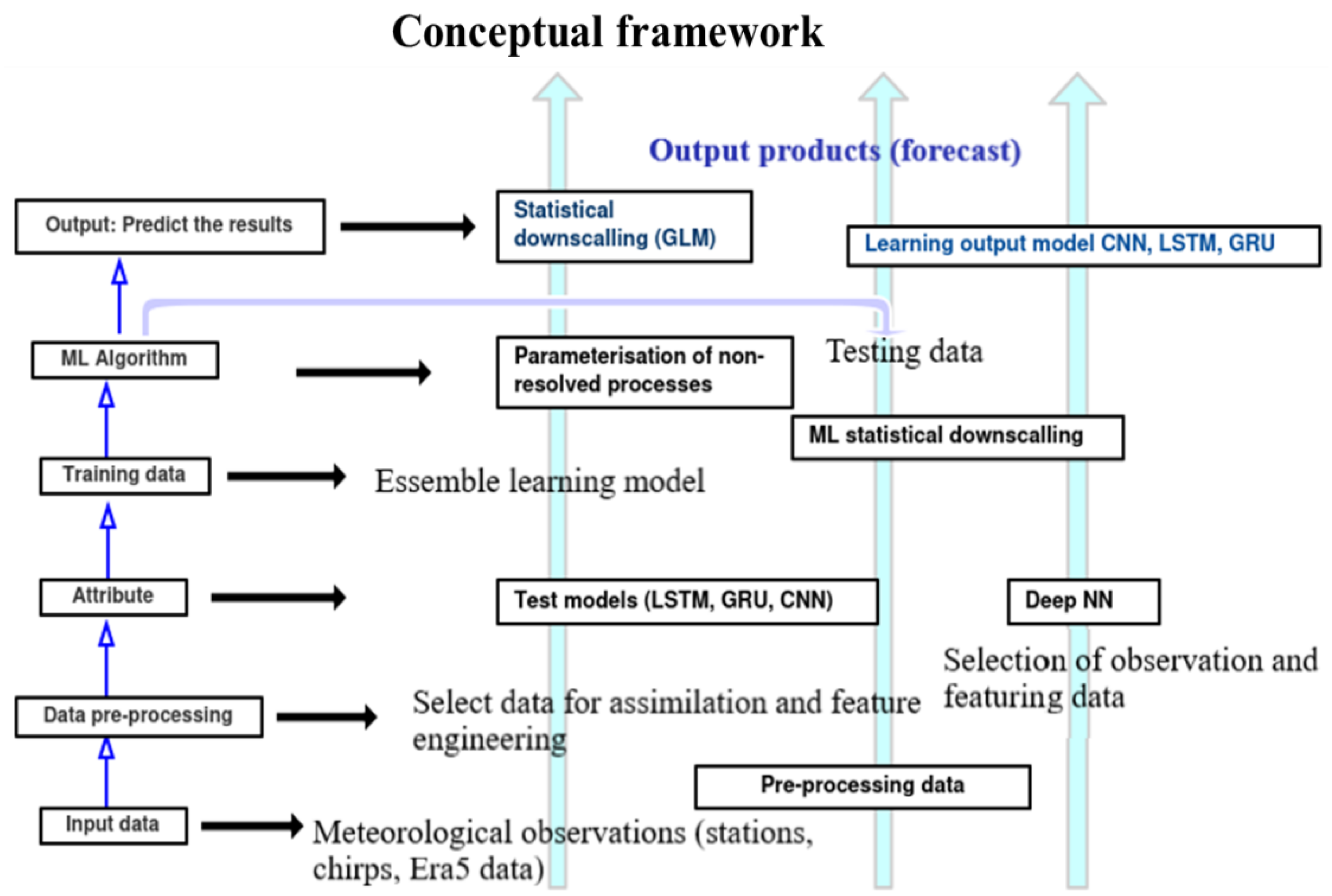
In this study, three deep learning algorithms (CNN, LSTM, and GRU) were employed, and a structured data preparation process was followed. This process encompassed data selection, checking, and filtering. Secondly, preprocessing was used for data testing, assimilation, and feature engineering. Subsequently, ensemble ML was conducted through model training, parameterization, and statistical downscaling. Each model underwent testing to assess its performance; the results were analyzed based on the learning model output (Figure 3).

3.2.2. Statistical Methods

In choosing the most suitable algorithm to predict different rainfall events accurately, it is advisable to utilize a linear statistical model. This model establishes a straight-line relationship between the dependent variable (Y) and one or more independent variables (X), as described below.
Y = β 0 + β 1 X + ε
X is the predictive variable (input data) to predict Y and ε is random variable. Y denotes the dependent variable, while X is the independent variable; β0 is the y-intercept, β1 is the slope of the line, and ε is the error term representing the difference between the actual rainfall and the predicted value. The LSTM architecture is one of the recurrent neural networks (RNNs) intended to solve the vanishing gradient issue with the conventional RNNs; a hyper parameter is essential in balancing the complexity and generalization in LSTM model optimization to achieve accurate predictions and preventing overfitting. It entails modifying learning rates, training epochs, and batch size, allowing an increased learning rate. In a variety of applications, the optimal performance is ensured by proper tuning. LSTM was employed to analyze weather parameters and make rainfall predictions based on input parameter values. In our study, the architecture underwent adjustment after a comprehensive hyper parameter tuning process.
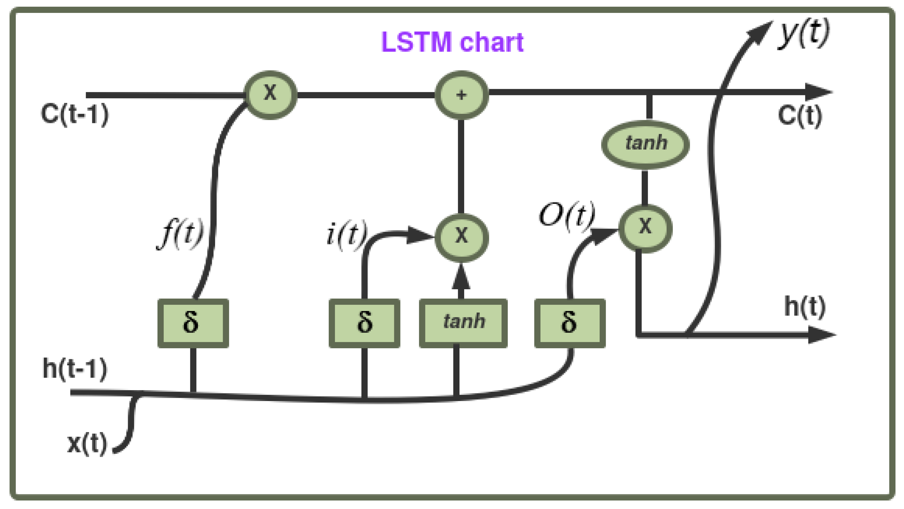
Regarding the neural network components, the vanishing gradient problem was solved with gated recurrent units. GRUs regulate the information flow through gating processes [64]. By deciding which data should be kept in the network’s internal state and which should be sent to the output, these gates help the model better represent dependencies for sequences of different lengths [66]. While training data, various procedures are adopted. With regard to the strategy of the batch normalization, which is a widely adopted technique that enables faster and more stable training of deep neural networks, it reduces the number of training epochs required for building deep networks [67,68]. With regard to the dense data layer, which enhances the performance of different neural network topologies during training and testing with varying optimization losses and activation functions, each neuron receives input from all of the neurons in the previous layer [69]. The artificial neural networks (ANNs) rely heavily on the activation function, which gives the model nonlinearity and allows it to recognize intricate patterns and relationships in the data. The rectified linear unit (ReLU) activation function was used in the deep learning model that was discussed by Srivastava. By using a regularization method for reducing overfitting and enhancing generalization performance in neural networks, we applied “dropout”. Over the course of training, a subset of layer outputs randomly drops out and a portion of the neurons in a layer are randomly deactivated; this mimics training several neural networks with various topologies concurrently [70]. A one-dimensional convolutional layer referred to as Conv1d in neural network terminology is usually used for sequences or time-series data and carries out convolution operations along one dimension. The output layer is responsible for producing the final prediction or output of the neural network based on the learned features from the preceding layers. Its structure and activation function are determined by the specific requirements of the task at hand. The LSTM incorporates several gates and activation functions to manage and update the cell state and hidden state; the suggested model makes use of sigmoid and tanh, which are the endemic activation functions of neural networks, and discusses an innovative technique to improve the outcomes in number of ways. It is calculated for an input gate It, Ot = output gate, δ = sigmoid, Ft = forget gate, Ct = candidate vector, Ct = cell state, and hidden state ℎt [71].
I t = s i g m o i d W t X t , h t 1 + b t
F t = s i g m o i d W f h t 1 , X t + b f
O t = s i g m o i d W o h t 1 , X t + b t
C t = tanh ( W c h t 1 , X ( t ) + b c )
C t = F t × C t 1 + I t × C t
h t = O t × tanh ( C t )  
As mentioned previously, the LSTM architecture itself makes use of the sigmoid and tanh functions; nevertheless, there are several issues with the activation functions that LSTM employs. The preceding section further provides this model’s challenges. Learning continues with neurons engaged throughout the training phase when the gradient is held at specific levels of backpropagation, hence avoiding the vanishing gradient problem [72]. To address the gradient issues that arise during backpropagation, sigmoid-weighted linear units were suggested, as these units multiply the input value by the sigmoid activation function. With this as its central concept, intensified LSTM was created. The cell state is a state created to retain historical data and simulate human brain decision making. LSTM uses tanh functions and sigmoid functions to update previous cell states when an operation is carried out. This is the point at which we genuinely removed outdated data and added current data. However, multiplying the input values by the forget and output gates was unusable as they determine input retention and prediction. As a result, it is evident that the input gate and candidate vector are crucial in maintaining the cell state vector, which the LSTM uses to absorb new data and perform analysis to forecast the output value given the current input. This is the basis for multiplying the input value by the candidate vector’s tanh function and the input gate’s sigmoid function [73].
Figure 4 shows the structural representation of the suggested intensified LSTM model. It is evident that the cyclical relationship between the input and hidden layer is captured by a more intricate structure in LSTM. It is possible to acquire the same output as an ordinary RNN [74] with an input Gate (I) function multiplied by the input; the forget gate is a sigmoid activation function; the candidate vector (C′) with tanh is the activation function multiplied by the input; the output gate (O) with tanh activation function; the hidden state (h) with hidden state vector; and the memory state (C) is with the memory state vector. The whole LSTM architecture is made up of the three input gates, which eliminates unnecessary information, while the output gate chooses what data to output. The input gate also chooses whether to allow new input; all these inputs operate within the range of 0 to 1. These three analog gates are based on the sigmoid function.
Hence, h(t) = O(t)⋅tanh C(t); the X(t) is the input at time step t, h(t) is the hidden state at time step t, C(t) is the cell state at time step t, I(t), F(t), and O(t) are the input and forget vectors and Y(t) is output gate vector, respectively. This model architecture is made up of three input gates, which eliminates unnecessary information while the output gate chooses what data to output. The input gate chooses whether to allow new input; all operate within the range of 0 to 1. These three analog gates are based on the sigmoid function [73].

3.2.3. Arithmetic Operations

The findings of the prediction accuracy were obtained using the data remaining for the training after the testing phase, which was based on the deep learning approach. The results show how effectively the suggested model would work to reduce all kinds of errors. The percentage of the dependent variable’s variance that can be predicted from the independent variables is the coefficient of determination. The mean absolute error (MAE) equation (8), the coefficient of determination equation (9), and the root mean square error (RMSE) equation (10) were the metrics validated to assess the models’ performances [43,63,75]. The coefficient of determination interprets the proportion of observed y variation that can be explained by the simple linear regression model attributed to an approximate linear relationship between y and x; it is denoted by R2. The mean absolute error (MAE) is a metric used to evaluate a regression model’s effectiveness, it measures the average absolute difference between the predicted values and the actual values in the dataset. The root mean square error is the “square root of the average of squared errors” [76].
M A E = 1 n i = 1 n y i y ^ i
R 2 = 1 i y i y ^ i 2 i y i y ¯ 2
R M S E = 1 n i = 1 n x i y i 2
where n is the sample size, xi is the model’s simulated daily rainfall, yi denotes the dataset’s i-th observed value, and y ^ is the predicted value.

4. Results

4.1. Training Dataset Development, Validation, and Rainfall Forecast

The use of ML algorithms in our study on rainfall data in Rwanda has become potentially significant for climate change predictions including the rainfall forecast. A dataset including a daily record of the weather parameters from 1983 to 2021 was used and accounted for record length, data continuity, and a contemporaneous period of observation. The consistency of the meteorological data was also validated. During data preprocessing, no missing values were detected. Parameters such as pressure, wind speed, relative humidity, and the maximum and minimum temperatures were used as inputs, while precipitation was the output. The training dataset comprised approximately 70% of the data from 1983 to 2009, the testing dataset covered ratio of 20% from 2010 to 2018, and the validation dataset comprised 10% from 2019 to 2021.

4.2. Model Performance on Rainfall Forecast

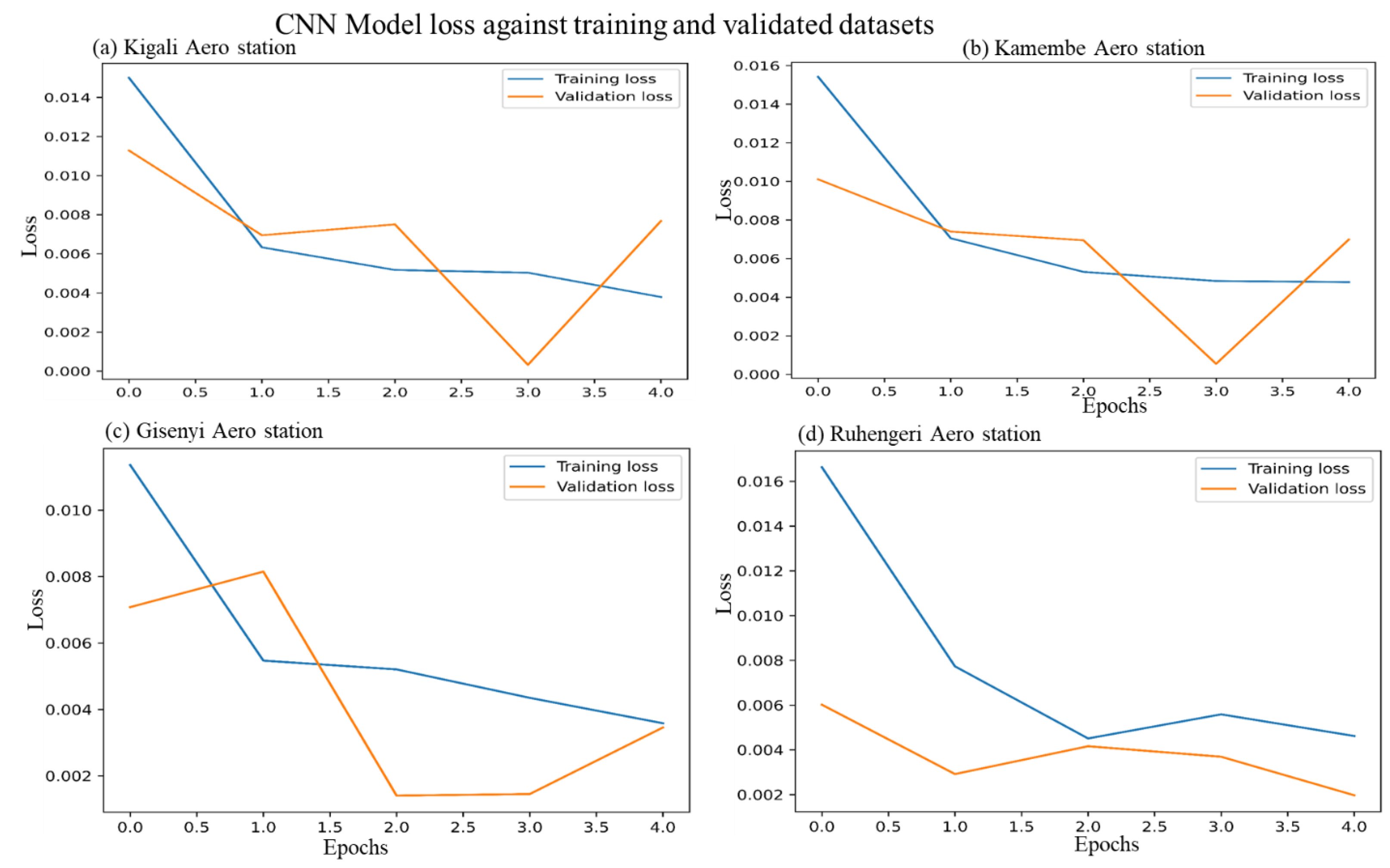
The loss plot of the rainfall forecast model throughout the training process was comparable for both the training and validation datasets. The three fundamental scoring metrics (RMSE, MAE, and R2) were used to assess the suggested model. Using these scoring metrics helps to evaluate the effectiveness of predictive models and offers valuable insights into various facets of model performance, including accuracy, error magnitude, and explanatory power. Comparing these metrics significantly contributes to validating and establishing the model’s predictive capabilities, thereby increasing confidence in its practical application. A 128-neuron long short-term memory model was used to present the experimental results. We evaluated the network’s prediction accuracy using data that were not included in the training phase, in addition to utilizing the suggested deep-learning-based daily rainfall prediction model. The performance of the proposed model during training and validation is shown in Figure 5. This figure presents the loss curves of the model over four epochs at four different synoptic weather stations including Kigali, Kamembe, Gisenyi, and Ruhengeri. The training loss (blue) decreases significantly, indicating successful learning from the training data, while the (orange) curve denotes the validation loss. The convergence of both loss curves without a significant increase in validation loss is indicative of good generalization and an absence of overfitting. We also assessed the suggested model’s prediction ability with a testing dataset; the outcomes are shown in Table 2, Table 3 and Table 4. Table 2 presents a comparison between the accuracies and RMSE of the predictive models, incorporating the statistical approaches, while Table 3 represents a determination coefficient with a high value on LSTM to all experiments across the stations. The MAE of our proposed system is compared with the aforementioned models, and the comparison is shown in Table 4.
During the testing and validation phase, the difference between the anticipated and actual outputs were minimized using backpropagation, hence reducing the error values. The error value represents the discrepancy between the actual and predicted values. Errors decreased gradually and stability was attained. The gradient continues throughout the suggested model, resulting in minimum losses. Losses were plotted against the number of epochs, showing a gradual decrease to about 0.005 at four epochs from around 0.008 at one epoch. The difference is in a continuously decreasing trend, demonstrating the suitability of the proposed model (Figure 5a–d).

4.3. LSTM Model Performance over Four Synoptic Stations

The RMSE of our proposed system is compared with the three different models (LSTM, GRU, and CNN), and the results are shown in Table 2. The RMSE values obtained for the LSTM, GRU, and CNN methods are 0.003, 0.008, and 0.007 at Kigali, 0.008, 0.010, and 0.007 at Kamembe, 0.007, 0.011, and 0.009 at Gisenyi, and 0.004, 0.007, and 0.006 at Ruhengeri Aero station, where Ruhengeri and Kigali have the lowest RMSE values across all models. Additionally, the LSTM model outperforms other models for all stations, showing a high R2 of 0.998 at Kamembe and Ruhengeri stations, as shown in Table 3, and the lowest MAE values of 0.003, 0.004, and 0.004 for Kigali, Kamembe, and Ruhengeri Aero stations, as shown in Table 4. Based on the above results, the LSTM model outperformed the other models across the four stations (Kigali, Kamembe, Gisenyi, and Ruhengeri). The CNN and GRU model test results and prediction performances can be found in Appendix A Figure A1a–d, Figure A2a–d, Figure A3a–d and Figure A4a–d respectively.
Through running the pairwise t-tests, we compared the performance of the LSTM, GRU, and CNN models based on metrics such as the MAE, R2, and RMSE. The results consistently showed that LSTM outperformed both the GRU and CNN across all metrics, with significant t-statistic values and low p-values. Table 5 indicates the statistical significance of the model. These findings support LSTM as the preferred model for rainfall prediction tasks due to its accuracy and effectiveness in precise forecasting applications.
To compute the outlier index, we divided the number of outliers by the total number of samples. This is a metric that quantifies the frequency of outliers in a dataset; the formula is expressed as:
O u t l i e r   I n d e x = N u m b e r   o f   O u t l i e r s T o t a l   n u m b e r   o f   s a m p l e s  
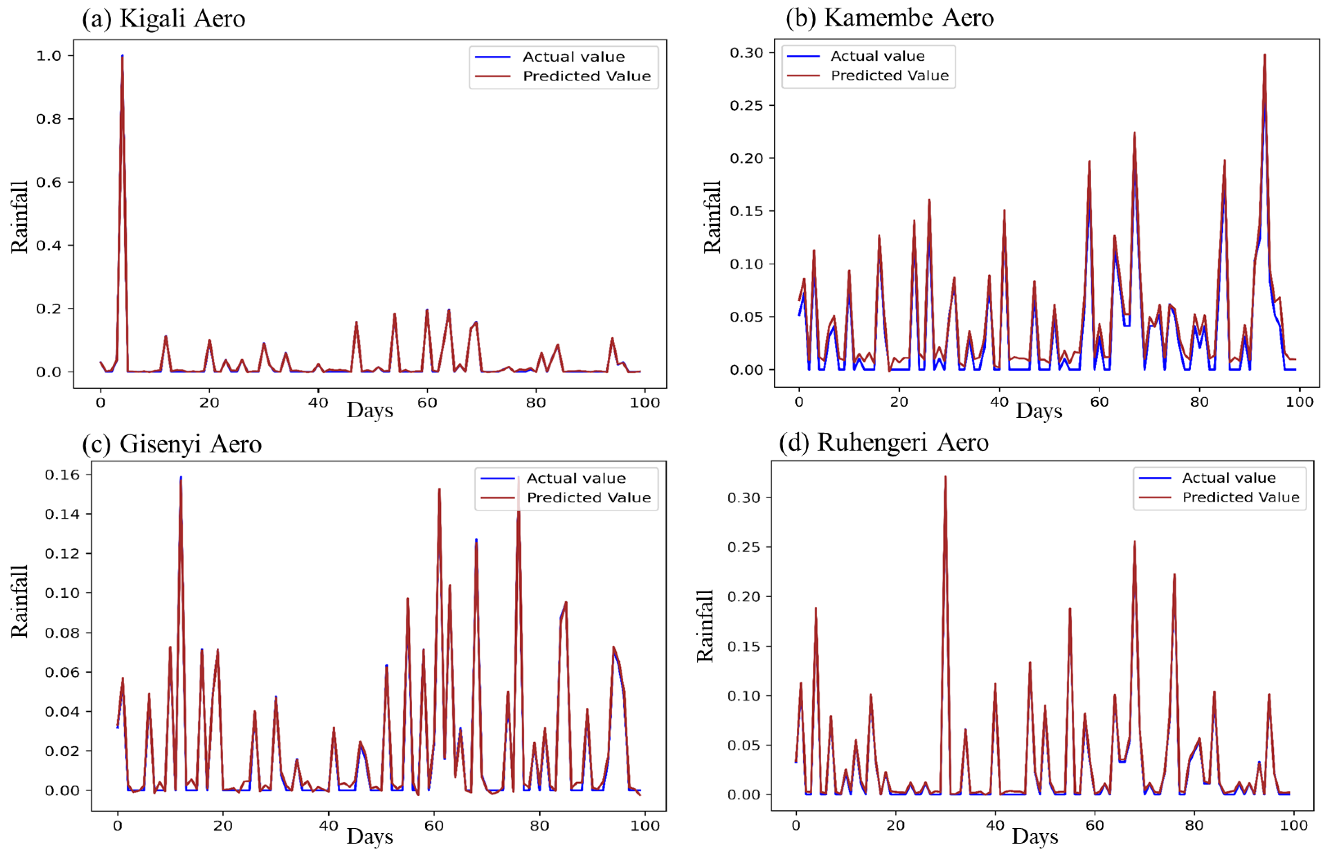
This method gives us a useful insight into the distribution of the data and possible anomalies by expressing the relative frequency of outliers within the sample as a standardized metric. Considering the outlier detection analysis conducted across the Kamembe Aero, Kigali Aero, Gisenyi Aero, and Ruhengeri Aero stations revealed outlier proportion indices of 0.07,0.17, 0.09, and 0.09, respectively (Figure 6).
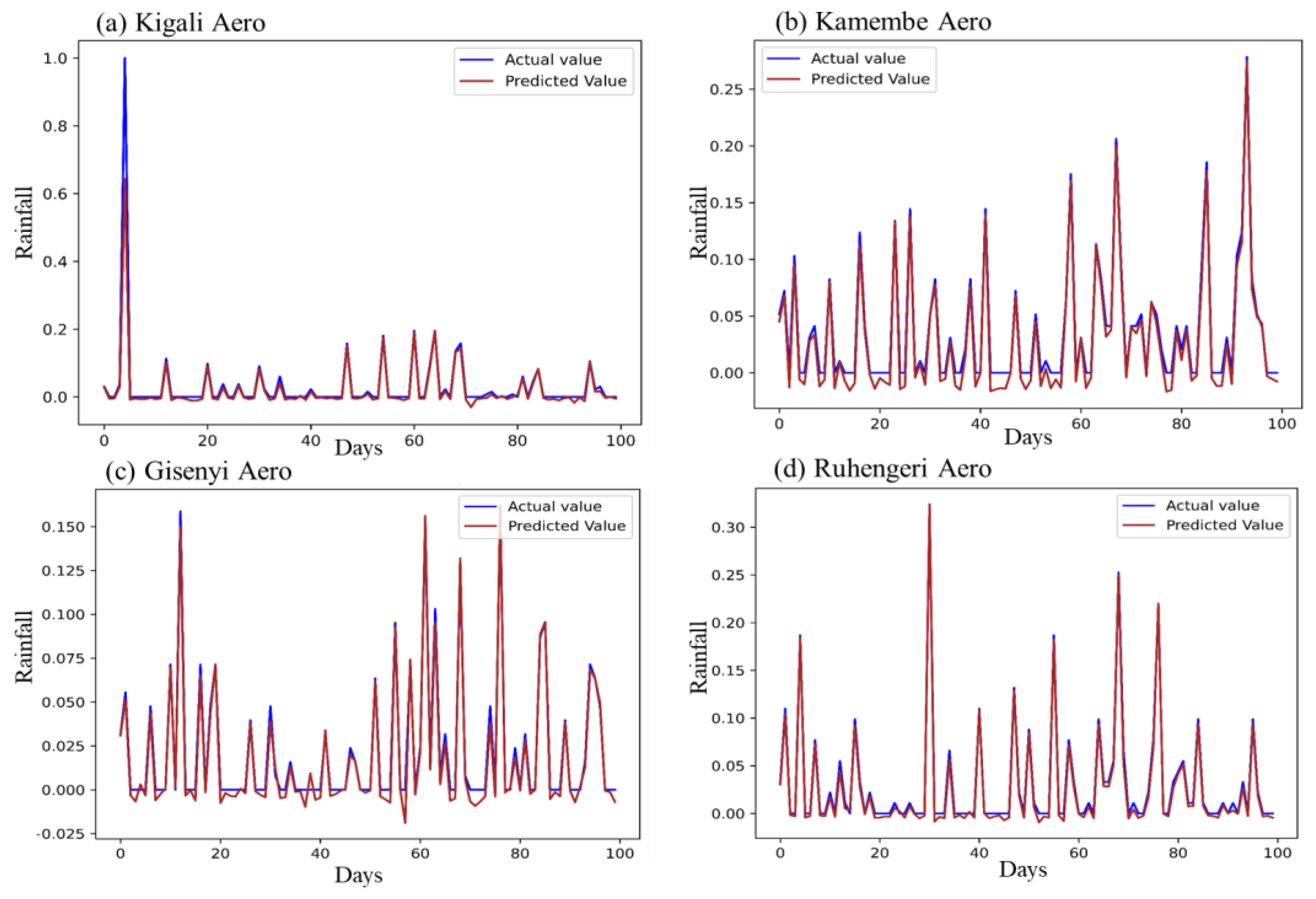
These outlier proportion indices, along with the evaluation of model performance metrics including RMSE, MAE, and R2, suggest that the prediction accuracy of the CNN and GRU models is impacted by the existence of outliers. Specifically, these outliers represent unconventional precipitation cases that deviate significantly from typical patterns. In contrast, the LSTM model showcased outstanding performance across all stations, even for stations with a high outlier proportion (Figure 7a,d).
Based on the method and data used, the findings demonstrate that the suggested methodology can predict average rainfall with high accuracy. The amount of average rainfall predicted by the suggested model is shown by the red line, while the actual amount measured by the rain gauge is represented by the blue line (Figure 7). The suggested model can therefore be used to forecast the amount of rain that will fall on a given day. The x- and y-axes represent the day and daily rainfall values, respectively, for the stations.
Over the training period, a decline in the learning rate is anticipated. We used the Adam optimizer to minimize the loss function during the training of neural networks. During this process, all models underwent training to fit a nonlinear dynamical model 100 times, and the loss function that we used is the mean squared error. The suggested model improves the findings in several ways by utilizing sigmoid and tanh, which are the endemic activation functions of neural networks. This section covers all the model performance results, comparisons, and validations of the recommended predictions. As the RMSE is used as a model performance, the computed RMSE is therefore plotted against the number of epochs for the intensified LSTM model. It is evident that the RMSE decreases to a minimum of 0.002 in the fourth epoch, but the network was further trained to achieve a good accuracy, learning rate, and loss minimization. At the last epoch, we obtained the RMSE as 0.005, with a loss validation of about 0.003 against epochs training at Kigali Aero and all other stations that have shown a promising result in predicting the rainfall event, and it fluctuates at around the same value for further epochs.
The results shown in this study highlight the extended opportunities afforded by the previously mentioned methods, which have recently emerged as crucial components of atmospheric science owing to their research potential and applications. The undeniable applicability of these methods in model prognosis suggests that machine learning techniques can effectively address a range of issues in meteorology and synoptic climatology. These include analyzing and identifying current circulation patterns, flooding, dynamic systems, solar radiation, wind, and other weather-related patterns.

5. Discussion

In our study, a Python library named “keras” was used to train the LSTM model on top of the Tensorflow backend. This procedure helped build, design, train, and deploy a neural network. The experiment showed statistically significant differences between the results of the methods used. When cross-validation was performed using “keras”, the results of the experiments were presented through a predictive algorithm. Prior to training, hyper parameter tuning is a crucial procedure, as hyper parameters such as the number of hidden layers, learning rate, number of hidden nodes in each layer, and dropout rate can significantly impact the model’s performance. Keras allows for the random selection of values from a range of hyper parametric numerical values [77]. Keras shows the number of epochs, which defines how many times the entire training dataset is processed during training, while other libraries may have default values for hyper-parameters leading to variations in model performance. Integrating with TensorFlow’s backend ensured scalability and performance; this makes it easier and more beneficial in experiments. It also provides high-level abstractions for building complex neural network architectures [78].
LSTM model outstrips other ML models (CNN and GRU) and enhances the accuracy of rainfall estimates in Rwanda (Figure 7) for a given day and over the next 100 days. This improvement in forecasting will help to mitigate climate-induced rainfall hazards in the country. As the best-performing model for the Rwanda’s rainfall forecast, the LSTM demonstrates a strong relationship between the observed and predicted data, building confidence in daily rainfall predictions. In rainfall forecasts, the LSTM, GRU, and CNN models offer distinct advantages. The GRU’s computational efficiency is notable, but it struggles with long-term dependencies [50]. Conversely, CNNs excel in spatial pattern recognition but lack the ability to capture complex temporal relationships critical for rainfall forecasting [51]. This study identifies LSTM as the optimal choice for rainfall prediction due to its ability to handle long-term dependencies, adapt to data time series, and accurately represent rainfall patterns, water resource, biodiversity, and natural conservation. Lately, the LSTM model has been used more in Africa’s agroecosystem management [79]. Being an agriculture-dependent country, Rwanda’s food and water security largely relies on the climatic conditions; many farmers uses rainfall-derived water sources for crop and livestock production [80]. Any deviations in the natural rainfall patterns in the country could significantly impact the marginal farming community, causing famine and poverty. Hence, the LSTM model has been found to enhance Rwanda’s preparedness ability for catastrophic events such as unpredicted rainfall, floods, and erosions and aid in nature preservation. Lately, climate change has also led to observable impacts, including both increased and decreased water levels in lakes and rivers, causing a loss of biodiversity in Rwanda [81].
Changes in climate have significantly reduced the country’s agricultural productivity, adversely affecting crops and exacerbating issues related to food security, public health, and livelihood nationwide [82]. Although the Government of Rwanda has implemented important measures [83], such as promoting climate-smart farming methods to increase resistance, drought-tolerant plants, sustainable land management strategies, and agroforestry systems, as well as strategic planning to reduce GHG emissions through various platforms and improved agriculture systems [82], challenges remain due to insufficient studies on improved mathematical modeling. Our approach of using machine learning algorithms such as LSTM for rainfall forecasting in Rwanda has significantly improved the predicting capabilities, accuracy, and the early warning system (EWS), providing information for natural disaster management. The ML techniques used by various scholars on the EWS often characterize the environmental conditions through better prediction and attributions of extreme rainfall and other events [84,85]. For instance, in places like Orissa and Kerala, where heavy rainfall can lead to property destruction and potential flooding, accurate rainfall prediction was a crucial concern for industries, the government, and risk management entities that required knowledge of the atmospheric conditions and predictive schemes to forecast future events [86]. The study in India highlighted the usefulness of mathematical approaches for rainfall prediction as a fundamental concern. However, the implementation of artificial neural networks (ANNs) brought a significant shift in decision making by emphasizing the better preparedness for disastrous events [77]. For example, the use of an ML algorithm successfully managed the impact of a flash flood in a small mountainous catchment, Anhe, in southwest of the Jiangxi province of China [87].
The model’s performance in our study shows implications for better preparedness and planning during natural disasters such as floods in Rwanda. The LSTM model has gained strong momentum in Rwanda’s rainfall forecasting as it introduces a data-driven approach based on a deep neural network. The deep neural network was meticulously built and evaluated to forecast rainfall events at four synoptic stations: Kigali Aero, Kamembe Aero, Gisenyi Aero, and Ruhengeri Aero. The data normalization technique we adopted in the deep neural network significantly improved prediction accuracy [88]. Hence, the LSTM model was proven to be a dependable rainfall forecasting tool by learning long-term dependencies between successive data series [73]. The nonlinearity and temporal dependency of rainfall data make the LSTM model suitable for learning in a complex modeling and dynamic environment. For instance, this model (ML algorithms) was applied for predicting daily rainfall events in Senegal, where several meteorological parameters, including the relative humidity, rainfall, and maximum and minimum temperatures were successfully predicted using LSTM [63]. This model has also been extensively applied in flood and drought predictions in Anhe, southwest of the Jiangxi province of China, where the model was found to be useful for better planning and preparedness for natural disasters. For Rwanda, although the LSTM model’s robustness is confirmed for the rainfall forecast, we are aware of the intricate nature of the climate system and the existence of nonlinear correlations between meteorological factors and rainfall patterns in East Africa. The LSTM model captures the hydro-metrological complexity and temporal sequential data, but the diversity of the terrains and microclimatic conditions in Rwanda often limits its ability to accurately represent the climate system relationships within the country. For instance, the steep and rocky terrains of western Rwanda experience notable rainfall events that usually cause significant erosion, mudslides, and landslides [89]. The spatial heterogeneity of rainfall over Rwanda, which increasing heavily from eastern low-lands to western highlands [90], further intensifies extremities of flooding and landslides [15]. These events damage societal well-being and foster an environment prone to pests and diseases [91]. Improved and high-resolution datasets are needed for better prediction models in the future.

6. Conclusions

This study has explored the effectiveness of utilizing the LSTM, CNN, and GRU machine learning algorithms for predicting rainfall patterns. Through extensive experimentation and analysis, this study has demonstrated that the algorithms used here would offer promising results in accurately forecasting rainfall events in Rwanda. The LSTM has typically demonstrated the ability to capture temporal and long-term dependencies, proven to be effective in modeling the dynamic nature of rainfall patterns, and outperforms other models, such as the CNN and GRU, showing strengths in handling spatial and temporal features and contributing to an accurate prediction ability. In contrast, the CNN and GRU require additional preprocessing (feature engineering) to handle time-series data adequately.
In addition, this paper highlights the significance of preprocessing methods, data availability, and quality in maximizing machine learning model performance. The predictive power of the LSTM, CNN, and GRU models is greatly enhanced by utilizing a variety of datasets and suitable feature engineering techniques. The LSTM model in rainfall forecasting for Rwanda has advanced the prediction of the past rainfall trajectory accurately. Its effectiveness is well-validated numerically. The comparisons were made using traditionally available machine learning algorithms. Hence, the LSTM machine learning technique marks a notable advancement for weather forecasting and disaster preparedness in Rwanda. LSTM can predict rainfall occurrences more accurately across the country, allowing decision makers to take proactive measures. However, an improved model accuracy is essential in the future with the availability of high-resolution datasets. The most essential components needed are high-resolution satellite data, soil moisture data, and land cover data, as well as expertise in the validation and verification of these data when running the models. Deploying and training the LSTM model across all stations in Rwanda can make it prone to overfitting, especially when trained on a small dataset. The predicted rainfall dataset can potentially aid in hydro-meteorological assessments, particularly in identifying drought, which is a significant agricultural concern in Rwanda, as well as flash floods within the river catchment areas.
Overall, the findings of this research highlight the potential of methodologies and the effectiveness of machine learning algorithms used for forecasting rainfall events in Rwanda. Comparing and evaluating deep learning models and ensuring accuracy and reliability in predicting rainfall events in Rwanda using different weather parameters are significant. By integrating cutting-edge methods such as LSTM into the current forecasting systems, stakeholders in different sectors, including agriculture, water resource management, and disaster preparedness, would greatly benefit in terms of decision making and mitigating weather-related risks. Nevertheless, more research is needed to investigate other potential model optimization avenues and to address issues like computational complexity and data scarcity in the future.

Author Contributions

J.K. (James Kagabo) conceptualization, methodology, formal analysis, writing—original draft; G.R.K. revision, supervision, visualization, J.K. (Jonah Kazora) conceptualization, methodology; C.N.S. review, software development and design; F.H. methodology. All authors have read and agreed to the published version of the manuscript.

Funding

This research received no external funding.

Institutional Review Board Statement

Not applicable.

Informed Consent Statement

Not applicable.

Data Availability Statement

All data used in this research are available, accessible freely upon reasonable request.

Acknowledgments

We would like to extend our gratitude to Rwanda Meteorology Agency (Meteo Rwanda) for the provision of data. James Kagabo would like to thank the Government of Rwanda (GoR) and the Peoples Republic of China through the Ministry of Finance and Commerce (MOFOCM) for providing a scholarship to pursue his M.Sc. in Atmospheric Sciences at the Nanjing University of Information Science and Technology (NUIST). Giri Raj Kattel would like to acknowledge the Longshan Professorship at NUIST. We also acknowledge the three anonymous reviewers who provided insightful comments for this paper.

Conflicts of Interest

The authors declare no conflicts of interest.

Appendix A

Figure A1. Validation of CNN model for predicting rainfall at synoptic weather stations in Rwanda.
Atmosphere 15 00691 g0a1
Figure A2. CNN model performance with testing dataset for rainfall prediction at different station.
Atmosphere 15 00691 g0a2
Figure A3. GRU model performance with testing dataset for rainfall prediction at different stations.
Atmosphere 15 00691 g0a3
Figure A4. GRU model performance with testing dataset for rainfall prediction at different stations.
Atmosphere 15 00691 g0a4

References

  1. Arnell, N.W.; Livermore, M.J.L.; Kovats, S.; Levy, P.E.; Nicholls, R.; Parry, M.L.; Gaffin, S.R. Climate and Socio-Economic Scenarios for Global-Scale Climate Change Impacts Assessments: Characterising the SRES Storylines. Glob. Environ. Chang. 2004, 14, 3–20. [Google Scholar] [CrossRef]
  2. Cazenave, A.; Le Cozannet, G. Sea Level Rise and Its Coastal Impacts. Earth Futur. 2014, 2, 15–34. [Google Scholar] [CrossRef]
  3. Singh, R.M.; Gupta, A. Water Pollution-Sources, Effects and Control Water Pollution-Sources, Effects and Control. Res. Gate 2017, 5, 1–17. [Google Scholar]
  4. Gahlawat, I.N.; Lakra, P. Global Climate Change and Its Effects. Integr. J. Soc. Sci. 2020, 7, 14–23. [Google Scholar]
  5. Nkomo, J.C.; Nyong, A.O.; Kulindwa, K. The Impacts of Climate Change in Africa. In The Stern Review on the Economics of Climate Change; LSE: London, UK, 2006; 51p. [Google Scholar]
  6. IPCC. Summary for Policymakers: Synthesis Report. Climate Change. 2023 Synthesis Report; Contribution of Working Groups I, II III to Sixth Assessment Reports; The Intergovernmental Panel on Climate Change: Geneva, Switzerland, 2023; pp. 1–34. [Google Scholar]
  7. Kattel, G.R. State of Future Water Regimes in the World’s River Basins: Balancing the Water between Society and Nature. Crit. Rev. Environ. Sci. Technol. 2019, 49, 1107–1133. [Google Scholar] [CrossRef]
  8. Adger, W.N.; Arnell, N.W.; Tompkins, E.L. Successful Adaptation to Climate Change across Scales. Glob. Environ. Chang. 2005, 15, 77–86. [Google Scholar] [CrossRef]
  9. Godfray, H.C.J.; Beddington, J.R.; Crute, I.R.; Haddad, L.; Lawrence, D.; Muir, J.F.; Pretty, J.; Robinson, S.; Thomas, S.M.; Toulmin, C. Food Security: The Challenge of Feeding 9 Billion People. Science 2010, 327, 812–818. [Google Scholar] [CrossRef]
  10. Aryal, J.P.; Manchanda, N.; Sonobe, T. Expectations for Household Food Security in the Coming Decades: A Global Scenario. In Future Foods; Elsevier: Amsterdam, The Netherlands, 2022; pp. 107–131. [Google Scholar]
  11. Zhang, Z.; Kattel, G.R.; Shang, Y.; Wang, G.; Chuai, X.; Wang, Q.; Cui, X.; Miao, L. Steady Decline in Food Self-Sufficiency in Africa from 1961 to 2018. Reg. Environ. Chang. 2023, 23, 79. [Google Scholar] [CrossRef]
  12. Cohen, B. Urbanization in Developing Countries: Current Trends, Future Projections, and Key Challenges for Sustainability. Technol. Soc. 2006, 28, 63–80. [Google Scholar] [CrossRef]
  13. Hove, M.; Ngwerume, E.; Muchemwa, C. The Urban Crisis in Sub-Saharan Africa: A Threat to Human Security and Sustainable Development. Stab. Int. J. Secur. Dev. 2013, 2, 7. [Google Scholar] [CrossRef]
  14. Douglas, I.; Alam, K.; Maghenda, M.; Mcdonnell, Y.; McLean, L.; Campbell, J. Unjust Waters: Climate Change, Flooding and the Urban Poor in Africa. Environ. Urban. 2008, 20, 187–205. [Google Scholar] [CrossRef]
  15. Mikova, K. Effect of Climate Change on Crop Production in Rwanda. Earth Sci. 2015, 4, 120. [Google Scholar] [CrossRef]
  16. Bakshi, B.; Nawrotzki, R.J.; Donato, J.R.; Lelis, L.S. Exploring the Link between Climate Variability and Mortality in Sub-Saharan Africa. Int. J. Environ. Sustain. Dev. 2019, 18, 206–237. [Google Scholar] [CrossRef]
  17. Nilsson, M.; Sie, A.; Muindi, K.; Bunker, A.; Ingole, V.; Ebi, K.L. Weather, Climate, and Climate Change Research to Protect Human Health in Sub-Saharan Africa and South Asia. Glob. Health Action 2021, 14 (Suppl. S1), 1984014. [Google Scholar] [CrossRef] [PubMed]
  18. Opoku, S.K.; Filho, W.L.; Hubert, F.; Adejumo, O. Climate Change and Health Preparedness in Africa: Analysing Trends in Six African Countries. Int. J. Environ. Res. Public Health 2021, 18, 4672. [Google Scholar] [CrossRef] [PubMed]
  19. Safari, B. Trend Analysis of the Mean Annual Temperature in Rwanda during the Last Fifty Two Years. J. Environ. Prot. 2012, 3, 538–551. [Google Scholar] [CrossRef]
  20. Ngarukiyimana, J.P.; Fu, Y.; Sindikubwabo, C.; Nkurunziza, I.F.; Ogou, F.K.; Vuguziga, F.; Ogwang, B.A.; Yang, Y. Climate Change in Rwanda: The Observed Changes in Daily Maximum and Minimum Surface Air Temperatures during 1961–2014. Front. Earth Sci. 2021, 9, 619512. [Google Scholar] [CrossRef]
  21. Safari, B.; Sebaziga, J.N.; Siebert, A. Evaluation of CORDEX-CORE Regional Climate Models in Simulating Rainfall Variability in Rwanda. Int. J. Climatol. 2022, 43, 1112–1140. [Google Scholar] [CrossRef]
  22. Guo, Z.; Chen, S.S.; Kattel, G.R.; Mkumbo, A.C.; Xiong, C.; Gao, Q.; Shen, Q. Scenario Analysis of Phosphorus Flow in Food Production and Consumption System in the Mwanza Region, Tanzania. Sci. Total Environ. 2023, 879, 162991. [Google Scholar] [CrossRef]
  23. Mazo, J. Climate Conflict: How Global Warming Threatens Security and What to Do about It; Routledge: Oxfordshire, UK, 2010; Volume 409. [Google Scholar]
  24. Haggag, M.; Kalisa, J.C.; Abdeldayem, A.W. Projections of Precipitation, Air Temperature and Potential Evapotranspiration in Rwanda under Changing Climate Conditions. Afr. J. Environ. Sci. Technol. 2016, 10, 18–33. [Google Scholar]
  25. Trisos, C.H.; Adelekan, I.O.; Totin, E.; Ayanlade, A.; Efitre, J.; Gemeda, A.; Kalaba, K.; Lennard, C.; Masao, C.; Mgaya, Y.; et al. Africa. In Climate Change 2022: Impacts, Adaptation, and Vulnerability; Contribution of Working Group II to the Sixth Assessment Report of the Intergovernmental Panel on Climate, Change; Pörtner, H.-O., Roberts, D.C., Tignor, M., Poloczanska, E.S., Mintenb, K., Eds.; IPCC: Geneva, Switzerland, 2022. [Google Scholar]
  26. Austin, K.G.; Beach, R.H.; Lapidus, D.; Salem, M.E.; Taylor, N.J.; Knudsen, M.; Ujeneza, N. Impacts of Climate Change on the Potential Productivity of Eleven Staple Crops in Rwanda. Sustainability 2020, 12, 4116. [Google Scholar] [CrossRef]
  27. Ayugi, B.O.; Chung, E.-S.; Zhu, H.; Ogega, O.M.; Babousmail, H.; Ongoma, V. Projected Changes in Extreme Climate Events over Africa under 1.5 °C, 2.0 °C and 3.0 °C global Warming Levels Based on CMIP6 Projections. Atmos. Res. 2023, 292, 106872. [Google Scholar] [CrossRef]
  28. Gitz, V.; Meybeck, A.; Lipper, L.; Young, C.; Braatz, S. Climate Change and Food Security: Risks and Responses; FAO: Rome, Italy, 2016. [Google Scholar] [CrossRef]
  29. MIDMAR. Disaster Management Plan; Ministry of Disaster Management and Refugee Affairs(MIDMAR): Kigali, Rwanda, 2012. [Google Scholar]
  30. Li, L.; Mind’je, R. Hydrogeological Hazard Susceptibility and Community Risk Perception in Rwanda: A Case Study of Floods and Landslides; Springer: Singapore, 2023. [Google Scholar] [CrossRef]
  31. Ngarukiyimana, J.P.; Fu, Y.; Yang, Y.; Ogwang, A. Dominant Atmospheric Circulation Patterns Associated with Abnormal Rainfall Events over Rwanda, East Africa. Int. J. Cliamtology 2017, 38, 187–202. [Google Scholar] [CrossRef]
  32. Trenberth, K.E. The Impact of Climate Change and Variability on Heavy Precipitation, Floods, and Droughts. Encycl. Hydrol. Sci. 2005, 17, 1–11. [Google Scholar]
  33. Ziervogel, G.; Johnston, P.; Matthew, M.; Mukheibir, P. Using Climate Information for Supporting Climate Change Adaptation in Water Resource Management in South Africa. Clim. Chang. 2010, 103, 537–554. [Google Scholar] [CrossRef]
  34. Wagesho, N.; Claire, M. Analysis of Rainfall Intensity-Duration-Frequency Relationship for Rwanda. J. Water Resour. Prot. 2016, 8, 706. [Google Scholar] [CrossRef]
  35. Wainwright, C.M.; Finney, D.L.; Kilavi, M.; Black, E.; Marsham, J.H. Extreme Rainfall in East Africa, October 2019–January 2020 and Context under Future Climate Change. Weather 2021, 76, 26–31. [Google Scholar] [CrossRef]
  36. Nibagwire, N.C. Climate Change and Natural Disasters in Africa; Case Study of Rwanda. Master’s Thesis, Pan African University, Yaoundé, Cameroun, 2016. [Google Scholar]
  37. Perera, D.; Seidou, O.; Agnihotri, J.; Rasmy, M.; Smakhtin, V.; Coulibaly, P.; Mehmood, H. Flood Early Warning Systems: A Review of Benefits, Challenges and Prospects; UNU-INWEH: Hamilton, ON, Canada, 2019. [Google Scholar]
  38. Umer, Y.; Ettema, J.; Jetten, V.; Steeneveld, G.-J.; Ronda, R. Evaluation of the WRF Model to Simulate a High-Intensity Rainfall Event over Kampala, Uganda. Water 2021, 13, 873. [Google Scholar] [CrossRef]
  39. Hosseini, F.S.; Choubin, B.; Mosavi, A.; Nabipour, N.; Shamshirband, S.; Darabi, H.; Haghighi, A.T. Flash-Flood Hazard Assessment Using Ensembles and Bayesian-Based Machine Learning Models: Application of the Simulated Annealing Feature Selection Method. Sci. Total Environ. 2020, 711, 135161. [Google Scholar] [CrossRef]
  40. Bochenek, B.; Ustrnul, Z. Machine Learning in Weather Prediction and Climate Analyses—Applications and Perspectives. Atmosphere 2022, 13, 180. [Google Scholar] [CrossRef]
  41. Mohammed, M.; Khan, M.B.; Bashie, E.B.M. Machine Learning: Algorithms and Applications; CRC Press: Boca Raton, FL, USA, 2016. [Google Scholar] [CrossRef]
  42. Sankalp, S.; Rao, U.M.; Patra, K.C.; Sahoo, S.N. Modeling Gated Recurrent Unit (GRU) Neural Network in Forecasting Surface Soil Wetness for Drought Districts of Odisha. In Modeling and Mitigation Measures for Managing Extreme Hydrometeorological Events Under a Warming Climate; Kasiviswanathan, K.S., Soundharajan, B., Patidar, S., He, J., Ojha, C.S.P., Eds.; Elsevier: Amsterdam, The Netherlands, 2023; Volume 14, pp. 217–229. [Google Scholar] [CrossRef]
  43. Endalie, D.; Haile, G.; Taye, W. Deep Learning Model for Daily Rainfall Prediction: Case Study of Jimma, Ethiopia. Water Supply 2022, 22, 3448–3461. [Google Scholar] [CrossRef]
  44. Aderyani, F.R.; Jamshid Mousavi, S.; Jafari, F. Short-Term Rainfall Forecasting Using Machine Learning-Based Approaches of PSO-SVR, LSTM and CNN. J. Hydrol. 2022, 614, 128463. [Google Scholar] [CrossRef]
  45. Dotse, S.Q. Deep Learning–Based Long Short-Term Memory Recurrent Neural Networks for Monthly Rainfall Forecasting in Ghana, West Africa. Theor. Appl. Climatol. 2023, 155, 0123456789. [Google Scholar] [CrossRef]
  46. Bai, Z.; Liu, Q.; Liu, Y. Groundwater Potential Mapping in Hubei Region of China Using Machine Learning, Ensemble Learning, Deep Learning and Automl Methods. Nat. Resour. Res. 2022, 31, 2549–2569. [Google Scholar] [CrossRef]
  47. Dtissibe, F.Y.; Ari, A.A.A.; Abboubakar, H.; Njoya, A.N.; Mohamadou, A.; Thiare, O. A Comparative Study of Machine Learning and Deep Learning Methods for Flood Forecasting in the Far-North Region, Cameroon. Sci. Afr. 2024, 23, e02053. [Google Scholar] [CrossRef]
  48. Oshodi, I. Machine Learning-Based Algorithms for Weather Forecasting. Int. J. Artif. Intell. Mach. Learn. 2022, 2, 12–20. [Google Scholar] [CrossRef]
  49. Hochreiter, S. The Vanishing Gradient Problem during Learning Recurrent Neural Nets and Problem Solutions. Int. J. Uncertain. Fuzziness Knowl. Based Syst. 1998, 6, 107–116. [Google Scholar] [CrossRef]
  50. Lechner, M.; Hasani, R. Learning Long-Term Dependencies in Irregularly-Sampled Time Series. arXiv 2020, arXiv:2006.04418. [Google Scholar]
  51. Puthran, R. Spatio-Temporal Analysis of Hybrid CNN-GRU Model for Prediction of Earthquake for Disaster Management. Int. J. Intell. Syst. Appl. Eng. 2024, 12, 270–281. [Google Scholar]
  52. Adhikari, U.; Pouyan Nejadhashemi, A.; Herman, M.R. A Review of Climate Change Impacts on Water Resources in East Africa. Trans. ASABE 2015, 58, 1493–1507. [Google Scholar] [CrossRef]
  53. Persello, C.; Wegner, J.D.; Hänsch, R.; Tuia, D.; Ghamisi, P.; Koeva, M.; Camps-Valls, G. Deep learning and earth observation to support the sustainable development goals: Current approaches, open challenges, and future opportunities. IEEE Geosci. Remote Sens. Mag. 2022, 10, 172–200. [Google Scholar] [CrossRef]
  54. GoR Green Growth and Climate Resilience; Republic of Rwanda: Kigali, Rwanda, 2011; 100p.
  55. Kazora, J.; Zhu, W.; Kyaw, T.O.; Sebaziga, J.N.; Rusanganwa, F.; Kagabo, J. Enhancement of East African Monsoon Long Rainfall (March to May) Variability from Weekly to Annual Scale by Climatic Extremes. Atmos. Clim. Sci. 2023, 13, 491–506. [Google Scholar] [CrossRef]
  56. Akayezu, P.; van Duren, I.C.; Groen, T.A.; Grueter, C.C.; Robbins, M.M. Abundance and Spatial Distribution of the Main Food Species for Mountain Gorillas in the Virunga Massif, Rwanda. Biodivers. Conserv. 2019, 28, 3597–3620. [Google Scholar] [CrossRef]
  57. Kelemen, M.; Virgala, I.; Kelemenová, T.; Mikova, L.; Frankovský, P.; Lipták, T.; Lörinc, M. Distance Measurement via Using of Ultrasonic Sensor. J. Autom. Control 2015, 3, 71–74. [Google Scholar]
  58. Funk, C.; Peterson, P.; Landsfeld, M.; Pedreros, D.; Verdin, J.; Shukla, S.; Husak, G.; Rowland, J.; Harrison, L.; Hoell, A.; et al. The Climate Hazards Infrared Precipitation with Stations—A New Environmental Record for Monitoring Extremes. Sci. Data 2015, 2, 150066. [Google Scholar] [CrossRef] [PubMed]
  59. Muhire, I.; Ahmed, F.; Elbasit, A. Spatio-Temporal Variations of Rainfall Erosivity in Rwanda. J. Soil Sci. Environ. Manag. 2015, 6, 72–83. [Google Scholar]
  60. Ayugi, B.; Tan, G.; Ullah, W.; Boiyo, R.; Ongoma, V. Inter-comparison of remotely sensed precipitation datasets over Kenya during 1998–2016. Atmos. Res. 2019, 225, 96–109. [Google Scholar] [CrossRef]
  61. Blum, A.G.; Zaitchik, B.; Alexander, S.; Wu, S.; Zhang, Y.; Shukla, S.; Alemneh, T.; Block, P. A Grand Prediction: Communicating and Evaluating 2018 Summertime Upper Blue Nile Rainfall and Streamflow Forecasts in Preparation for Ethiopia’s New Dam. Front. Water 2019, 1, 3. [Google Scholar] [CrossRef]
  62. Jonah, K.; Wen, W.; Shahid, S.; Ali, M.A.; Bilal, M.; Habtemicheal, B.A.; Iyakaremye, V.; Qiu, Z.; Almazroui, M.; Wang, Y.; et al. Spatiotemporal variability of rainfall trends and influencing factors in Rwanda. J. Atmos. Sol. Terr. Phys. 2021, 219, 105631. [Google Scholar] [CrossRef]
  63. Nyasulu, C.; Diattara, A.; Traore, A.; Deme, A.; Ba, C. Towards Resilient Agriculture to Hostile Climate Change in the Sahel Region: A Case Study of Machine Learning-Based Weather Prediction in Senegal. Agriculture 2022, 12, 1473. [Google Scholar] [CrossRef]
  64. Tang, L.; Gao, W.; Xue, L.; Zhang, G.; Guo, J. Climatological Characteristics of Hydrometeors in Precipitating Clouds over Eastern China and Their Relationship with Precipitation Based on ERA5 Reanalysis. J. Appl. Meteorol. Climatol. 2023, 62, 625–641. [Google Scholar] [CrossRef]
  65. Davey, R. Scientists Report a Novel Method for Detecting Ice on Wind Turbines; AZoM: Manchester, UK, 2022. [Google Scholar]
  66. Cho, K.; Van Merriënboer, B.; Gulcehre, C.; Bahdanau, D.; Bougares, F.; Schwenk, H.; Bengio, Y. Learning Phrase Representations Using RNN Encoder-Decoder for Statistical Machine Translation. arXiv 2014, arXiv:1406.1078. [Google Scholar]
  67. Santurkar, S.; Tsipras, D.; Ilyas, A.; Madry, A. How Does Batch Normalization Help Optimization? In Proceedings of the Advances in Neural Information Processing Systems 31: Annual Conference on Neural Information Processing Systems 2018, NeurIPS 2018, Montreal, QC, Canada, 3–8 December 2018. [Google Scholar]
  68. Schilling, F. The Effect of Batch Normalization on Deep Convolutional Neural Networks. Master’s Thesis, KTH Royal Institute of Technology, Stockholm, Sweden, 2016. [Google Scholar]
  69. Javid, A.M.; Das, S.; Skoglund, M.; Chatterjee, S. A Relu Dense Layer to Improve the Performance of Neural Networks. In ICASSP 2021–2021 IEEE International Conference on Acoustics, Speech and Signal Processing (ICASSP); IEEE: New York, NY, USA, 2021; pp. 2810–2814. [Google Scholar]
  70. Srivastava, N.; Hinton, G.; Krizhevsky, A.; Sutskever, I.; Salakhutdinov, R. Dropout: A Simple Way to Prevent Neural Networks from Overfitting. J. Mach. Learn. Res. 2014, 15, 1929–1958. [Google Scholar]
  71. Kim, T.; Kim, H.Y. Forecasting Stock Prices with a Feature Fusion LSTM-CNN Model Using Different Representations of the Same Data. PLoS ONE 2019, 14, e0212320. [Google Scholar] [CrossRef] [PubMed]
  72. Bellec, G.; Scherr, F.; Hajek, E.; Salaj, D.; Legenstein, R.; Maass, W. Biologically Inspired Alternatives to Backpropagation through Time for Learning in Recurrent Neural Nets. arXiv 2019, arXiv:1901.09049. [Google Scholar]
  73. Abed, M.; Imteaz, M.A.; Ahmed, A.N.; Huang, Y.F. Application of Long Short-Term Memory Neural Network Technique for Predicting Monthly Pan Evaporation. Sci. Rep. 2021, 11, 20742. [Google Scholar] [CrossRef] [PubMed]
  74. Yu, Y.; Si, X.; Hu, C.; Zhang, J. A Review of Recurrent Neural Networks: LSTM Cells and Network Architectures. Neural Comput. 2019, 31, 1235–1270. [Google Scholar] [CrossRef] [PubMed]
  75. Hu, H.; Ayyub, B.M. Machine Learning for Projecting Extreme Precipitation Intensity for Short Durations in a Changing Climate. Geosciences 2019, 9, 209. [Google Scholar] [CrossRef]
  76. Bangdiwala, S.I. Regression: Simple Linear. Int. J. Inj. Contr. Saf. Promot. 2018, 25, 113–115. [Google Scholar] [CrossRef]
  77. Poornima, S.; Pushpalatha, M. Prediction of Rainfall Using Intensified LSTM Based Recurrent Neural Network with Weighted Linear Units. Atmosphere 2019, 10, 668. [Google Scholar] [CrossRef]
  78. Vasilev, I.; Slater, D.; Spacagna, G.; Roelants, P.; Zocca, V. Python Deep Learning: Exploring Deep Learning Techniques and Neural Network Architectures with Pytorch, Keras, and TensorFlow; Packt Publishing Ltd.: Birmingham, UK, 2019. [Google Scholar]
  79. Houmma, I.H.; El Mansouri, L.; Gadal, S.; Garba, M.; Hadria, R. Modelling Agricultural Drought: A Review of Latest Advances in Big Data Technologies. Geomat. Nat. Hazards Risk 2022, 13, 2737–2776. [Google Scholar] [CrossRef]
  80. Bezu, S.; Demissie, T.; Abebaw, D.; Mungai, C.; Samuel, S.; Radeny, M.A.O.; Huyer, S.; Solomon, D. Climate Change, Agriculture and International Migration Nexus: African Youth Perspective; CCAFS Working Paper; CGIAR Research Program on Climate Change, Agriculture and Food Security (CCAFS): Wageningen, The Netherlands, 2020. [Google Scholar]
  81. Mukanyandwi, V.; Nahayo, L.; Hakorimana, E.; Gasirabo, A.; Otgon, S. Review on Water Resources Management and Key Threats in Rwanda, East Africa. J. Water Secur. 2018, 4, jws2018003. [Google Scholar] [CrossRef]
  82. Mutabazi, A. Assessment of Operational Framework Related to Climate Change in Rwanda; Rwanda Environment Management Authority: Kigali, Rwanda, 2010; 41p. [Google Scholar]
  83. Taremwa, N.K.; Gashumba, D.; Butera, A.; Ranganathan, T. Climate Change Adaptation in Rwanda through Indigenous Knowledge Practice. J. Soc. Sci. 2016, 46, 165–175. [Google Scholar] [CrossRef]
  84. Mohammed, M.; Kolapalli, R.; Golla, N.; Maturi, S.S. Prediction of Rainfall Using Machine Learning Techniques. Int. J. Sci. Technol. Res. 2020, 9, 3236–3240. [Google Scholar]
  85. Frame, J.M.; Kratzert, F.; Klotz, D.; Gauch, M.; Shalev, G.; Gilon, O.; Qualls, L.M.; Gupta, H.V.; Nearing, G.S. Deep Learning Rainfall–Runoff Predictions of Extreme Events. Hydrol. Earth Syst. Sci. 2022, 26, 3377–3392. [Google Scholar] [CrossRef]
  86. Mall, R.K.; Kumar, R.; Bhatla, R. Climate Change and Disaster in India. J. South Asian Disaster Stud. 2011, 4, 27–76. [Google Scholar]
  87. Wu, J.; Liu, H.; Wei, G.; Song, T.; Zhang, C.; Zhou, H. Flash Flood Forecasting Using Support Vector Regression Model in a Small Mountainous Catchment. Water 2019, 11, 1327. [Google Scholar] [CrossRef]
  88. Zintgraf, L.M.; Cohen, T.S.; Adel, T.; Welling, M. Visualizing Deep Neural Network Decisions: Prediction Difference Analysis. arXiv 2017, arXiv:1702.04595. [Google Scholar]
  89. Hafashimana, N. Modelling the Effects of Land Use/Cover Change and Rainfall Variability on Landslide Hazards: The Case of Nyabihu District, Rwanda. Master’s Dissertation, University of Botswana, Gaborone, Botswana, 2020. [Google Scholar]
  90. Nkurunziza, I.; Guirong, T.; Ngarukiyimana, J.P.; Sindikubwabo, C. Influence of the Mascarene High on October-December Rainfall and Their Associated Atmospheric Circulation Anomalies over Rwanda. J. Environ. Agric. Sci. 2019, 20, 1–20. [Google Scholar]
  91. Patz, J.A.; Grabow, M.L.; Limaye, V.S. When It Rains, It Pours: Future Climate Extremes and Health. Ann. Glob. Health 2014, 80, 332–344. [Google Scholar] [CrossRef]
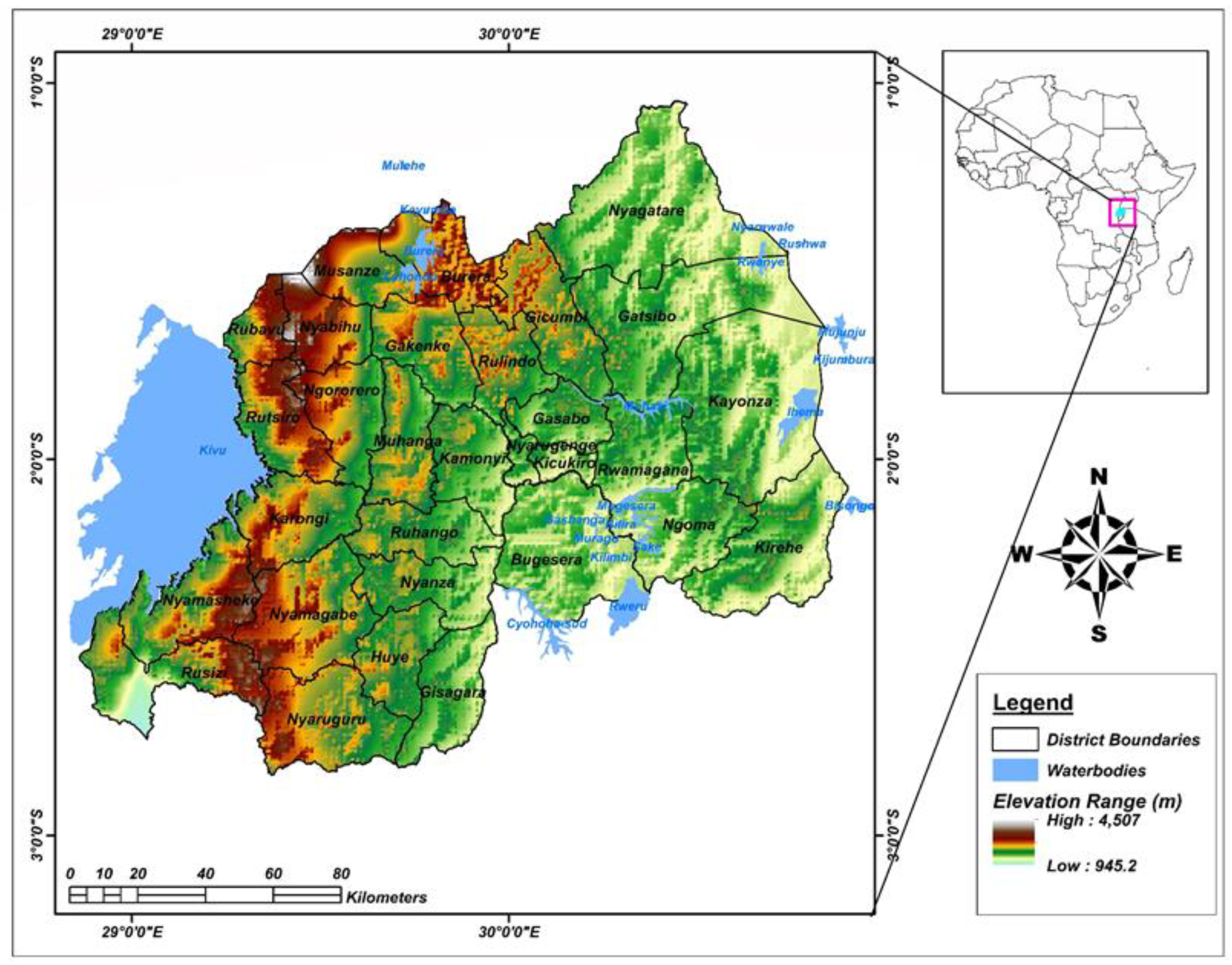
Figure 1. Geographical map of Rwanda with district boundaries, waterbodies, and elevation.
Atmosphere 15 00691 g001
Figure 2. Spatial climatological of variation over Rwanda. (a) Temperature (°C) variation and (b) rainfall (mm) distribution from 1981 to 2019.
Atmosphere 15 00691 g002
Figure 3. Conceptual framework that indicates data preprocessing and testing for the machine learning algorithm [65].
Atmosphere 15 00691 g003
Figure 4. LSTM flow chart showing input and output gates.
Atmosphere 15 00691 g004
Figure 5. Illustration of LSTM model loss against training and validated datasets at the (a) Kigali, (b) Kamembe, (c) Gisenyi, and (d) Ruhengeri Aero stations, respectively.
Atmosphere 15 00691 g005
Figure 6. Outlier distribution across stations covered by the study.
Atmosphere 15 00691 g006
Figure 7. LSTM model performance with the testing dataset for rainfall (mm) prediction at different stations, namely (a) Kigali Aero, (b) Kamembe Aero station, (c) Gisenyi Aero station, and (d) Ruhengeri Aero station, with best performance.
Atmosphere 15 00691 g007
Table 1. Selected stations with their latitude and longitude locations that were used in this study.
StationLatitudeLongitude
Kigali Aero−1.95°30.11°
Kamembe Aero−2.46°28.91°
Gisenyi Aero−1.68°29.26°
Ruhengeri Aero−1.48°29.61°
Table 2. Model evaluation comparing LSTM, GRU, and CNN by RMSE on the testing dataset; this table proposes the best performing model based on RMSE.
Model/StationKigali AeroKamembe AeroGisenyi AeroRuhengeri AeroAvg
LSTM0.0030.0080.0070.0040.005
GRU0.0080.0100.0110.0070.009
CNN0.0070.0070.0090.0060.007
Table 3. Testing dataset model evaluation comparing LSTM, GRU, and CNN by R2; this table proposes the best performing model based on R2.
Model/StationKigali AeroKamembe AeroGisenyi AeroRuhengeri Aero
LSTM0.9970.9980.9970.998
GRU0.9700.9850.9590.986
CNN0.9830.9890.9960.997
Table 4. Testing dataset model evaluation comparing LSTM, GRU, and CNN by MAE; this table proposes the best performing model based on MAE.
Model/StationKigali AeroKamembe AeroGisenyi AeroRuhengeri Aero
LSTM0.0030.0040.0090.004
GRU0.0050.0060.0050.006
CNN0.0040.0080.0070.007
Table 5. Comparing t-tests and p-values across various metrics between the LSTM model and other models, highlighting the efficacy of model’s statistical significance.
ModelLSTM vs. CNNLSTM vs. GRU
MetricsRMSEMAER2RMSEMAER2
p value1.43 × 10−2722.80 × 10−2753.83 × 10−2472.08 × 10−2742.80 × 10−2751.92 × 10−256
t test−4,891,431,684,499,790.00−6,917,529,027,641,070.00189,151,184,349,557.00−6,187,226,056,853,390.006,917,529,027,641,070.00621,496,748,577,125.00
Disclaimer/Publisher’s Note: The statements, opinions and data contained in all publications are solely those of the individual author(s) and contributor(s) and not of MDPI and/or the editor(s). MDPI and/or the editor(s) disclaim responsibility for any injury to people or property resulting from any ideas, methods, instructions or products referred to in the content.