Article

Development of X-Band Geophysical Model Function for Sea Surface Wind Speed Retrieval with ASNARO-2

1
Department of Marine Resources and Energy, Tokyo University of Marine Science and Technology, Tokyo 1088477, Japan
2
Renewable Energy Division, Tokyo Electric Power Services Company, Limited (TEPSCO), Tokyo 1350062, Japan
*
Author to whom correspondence should be addressed.
Atmosphere 2024, 15(6), 686; https://doi.org/10.3390/atmos15060686
Submission received: 17 April 2024 / Revised: 24 May 2024 / Accepted: 1 June 2024 / Published: 4 June 2024
(This article belongs to the Special Issue Satellite Remote Sensing Applied in Atmosphere (2nd Edition))

Abstract

:
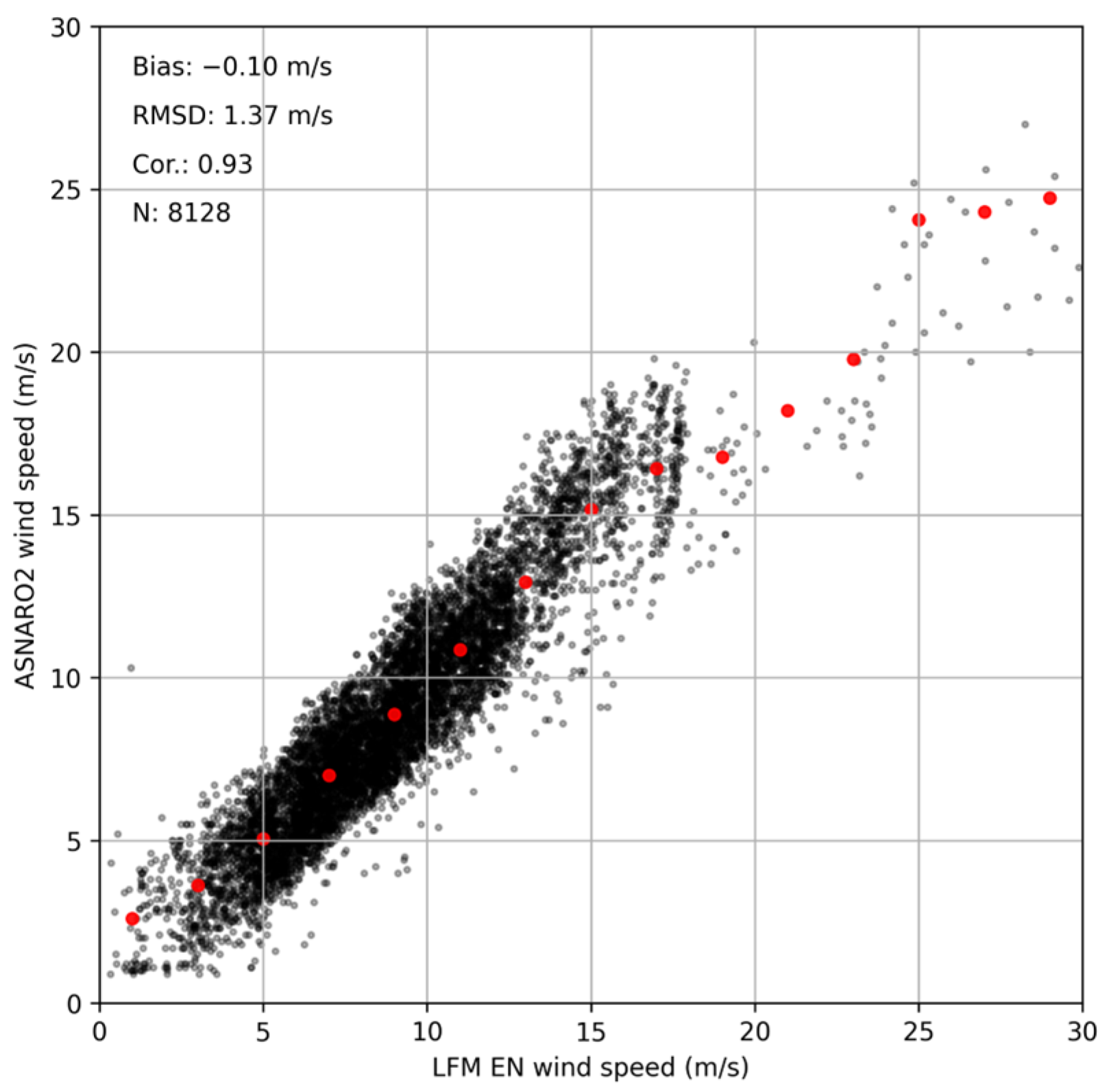
In the present study, a new geophysical model function (GMF) is developed for the X-band synthetic aperture radar (SAR) on board the Advanced Satellite with New System Architecture for Observation-2 (ASNARO-2) to retrieve accurate offshore wind speeds. Equivalent neutral wind speeds based on the local forecast model (LFM) are employed as reference wind vectors, and 12,259 matching points from 502 SAR images obtained with horizontal transmitting, horizontal receiving polarization around Japan are collected. To ensure convergence of the calculation, 8129 points are selected from the matching points to determine the basic formula for the GMF and 23 coefficients based on the relationships among the normalized radar cross section, wind speed, incidence angle, and relative wind direction. Compared with the reference wind speeds, the GMF wind speeds showed reproducibility with a bias of −0.10 m/s and an RMSD of 1.37 m/s. Additionally, it can be confirmed that the retrieved wind speed has the bias of 0.03 and the RMSD of 1.68 m/s when compared to the in situ wind speed from the Kuroshio Extension Observatory (KEO) buoy. The accuracy of these retrieved wind speeds is comparable to previous studies, and it is indicated that the developed GMF can be used to retrieve offshore winds from ASNARO-2 images.

1. Introduction

Synthetic aperture radars (SARs) using active microwaves on board sun-synchronous, near-polar-orbit satellites have been utilized for sea surface wind speed retrievals for several decades. A SAR measures the amount of radar backscatter from the sea surface. The backscattered normalized radar cross section (NRCS) can be expressed empirically as a function of the wind speed and direction at a height of 10 m above the sea surface, the incidence angle, the relative azimuth angle, the radar frequency, and the polarization. To retrieve the sea surface wind speed from SARs, a geophysical model function (GMF) has been utilized that is based on the relationship among these parameters. The European Space Agency began operations using the European Remote Sensing Satellite-1 (ERS-1) in 1991 and its successor, the ERS-2, in 1995. C-band (4–8 GHz) active microwave instruments on board the ERS-1 and ERS-2 have contributed to the development of C-band GMFs, CMOD4 [1], CMOD_IFR2 [2], CMOD5 [3], and CMOD5.N [4]. The most recent sea surface wind vector products obtained by the Advanced Scatterometers (ASCATs) use the latest C-band GMF, CMOD7 [5]. These GMFs have been applied to retrieve the wind speed with C-band SARs on board the European satellites ERS-1 [6], ERS-2 [6,7,8], Envisat [8,9,10,11,12,13], and Sentinel-1 [14], and these previous studies reported RMSEs of 0.9–1.8 m/s and 0.5–2.4 m/s in wind speed for offshore and coastal areas, respectively. Furthermore, using these C-band GMFs, wind speed data obtained using the Canadian satellites Radarsat-1 and Radarsat-2 have been validated with an RMSE of 1.5–2.5 m/s [15]. C-band GMFs prior to CMOD7 were intended for VV polarization, but GMFs have been improved that can be applied to HH polarization as well as VV polarization [16,17,18]. Furthermore, neural networks have been proposed to acquire wind speeds without GMF [19], but this method could be applied only to satellites with large amounts of archived images (e.g., Sentinel-1). An L-band (1–2 GHz) GMF had also been developed to retrieve the sea surface wind speed using the Advanced Land Observing Satellite (ALOS) [20].
The NRCS with the same bands should theoretically show the same values for the same incidence angle, relative wind direction, and wind speed. However, it is not necessarily the same NRCS value in all satellites. This may have something to do with the radiometric calibration, but this paper does not deal with the accuracy of the calibration itself. In fact, in the X-band (8–12 GHz) GMFs, XMOD1 [21] and XMOD2 [22] developed by TerraSAR-X and TanDEM-X and the GMF, which was improved by COSMO-SkyMed [23], have different characteristics of NRCS. The Advanced Satellite with New System ARchitecture for Observation-2 (ASNARO-2), which was developed by NEC cooperation and the Institute for Unmanned Space Experiment Free Flyer (USEF), is another satellite with characteristics of NRCS that differ from existing X-band satellites. The specifications of ASANRO-2 are shown in Table 1. Differences in NRCSs between ASNARO-2 and the other X-band SAR are compared in the Discussion. GMFs are developed based on characteristics of NRCS, so existing X-band GMFs cannot be applied to ASNARO-2. Therefore, a new GMF with the same or better accuracy than the previous GMF is necessary to retrieve offshore wind speed from ASNARO-2 images.

2. Data and Basic Formulas for GMF

2.1. SAR Images Obtained by ASNARO-2

A total of 502 ASNARO-2 ScanSAR mode images were obtained with horizontal transmitting, horizontal receiving (HH) polarization. The observation period was from June 2019 to January 2021, and the target areas around Japan are shown in Figure 1. The digital numbers (DNs) representing radar backscatter are obtained from level 1.1 images. The images cover an approximately 50 × 50 km square area along the track of the satellite. A total of 12,259 points were first identified to match the local forecast model (LFM) grids in these SAR images. The appearance frequency of relative wind directions for these matching points are shown in Figure 2. The relative wind direction (radar azimuth angle minus LFM wind direction) range includes the upwind, crosswind, and downwind directions.
First, the DNs from an image are converted to the NRCS using
σ 0 = 10   l o g 10 D N 2 + C F
where σ 0 is the NRCS (dB), and CF is a calibration factor of −40 dB. The NRCS is resampled by the weighted average method within a 500 m search radius.

2.2. Local Forecast Model and Sea Surface Temperature

The LFM is a numerical weather prediction model with a horizontal grid spacing of about 2 km provided by the Japan Meteorological Agency (JMA). The hourly LFM wind speed and wind direction by an objective analysis process are employed as reference wind vectors for the developing of the GMF. It is well known that the vertical wind speed profile depends on atmospheric stability. In order to be applicable to variable atmospheric stability conditions, the GMF is designed to retrieve the equivalent neutral wind (ENW) speed assuming neutral atmospheric conditions. The LFM wind speed at a height of 10 m is converted to the ENW speed based on the Monin–Obukhov similarity theory using the LKB code [24]. The LKB code was originally written to calculate the ENW speed from the actual wind speed. In this study, the code is used inversely with air temperature and relative humidity obtained from the LFM, and the sea surface temperature (SST) from the Operational Sea Surface Temperature and Ice Analysis (OSTIA) [25].

2.3. In Situ Wind Vectors Obserbed in the KEO Buoy

The National Oceanic and Atmospheric Administration (NOAA) Kuroshio Extension Observatory (KEO) buoy is located in the recirculation gyre region south of the Kuroshio Extension at 32.4° N, 144.6° E, as shown in Figure 1. The wind vectors are measured at 4 m height above the sea surface on the buoy. The in situ wind speed is compared with the retrieved wind speed from ASNARO-2 images to evaluate the developed GMF. Before the comparison, the in situ wind speed at 4 m height is converted to ENW speed at 10 m height using the LKB code as described above.

2.4. Formula for GMF

Bragg scattering is dominant when microwaves are backscattered from a rough sea surface because of resonance between the microwaves and short surface gravity and capillary waves. For a sea surface wavelength, L, a radar incidence angle, θ, and a microwave wavelength, λ, the main contribution to the backscattered microwave strength is given by
L = n λ 2 sin θ          n = 1,2 ,   3 , .
The angle between the radar azimuth and the wind direction also significantly affects the backscattered microwave strength. The scattering strength is maximized when the radar azimuth angle is toward the wind direction (upwind) and is minimized when the angle is perpendicular to the wind direction (crosswind). This can be expressed as
σ 0 = A 0 1 + A 1 cos φ + A 2 cos 2 φ   ( Linear unit )
where σ 0 is the NRCS indicating the scattering strength, φ is the relative wind direction, and A 0 , A 1 , and A 2 are functions of the wind speed and incidence angle.

3. Development of the GMF

3.1. Determination of A 0

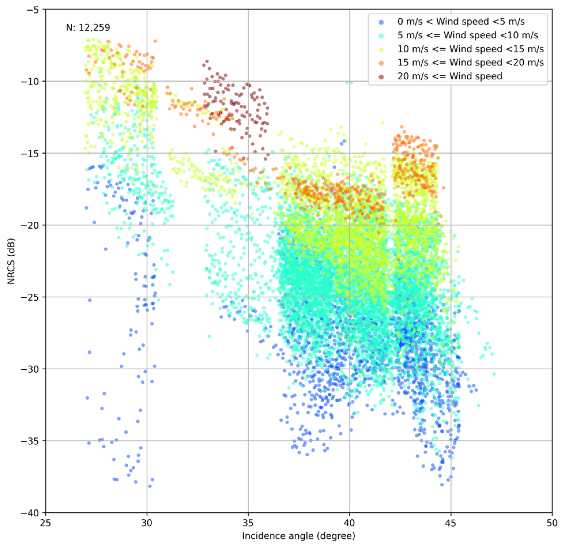
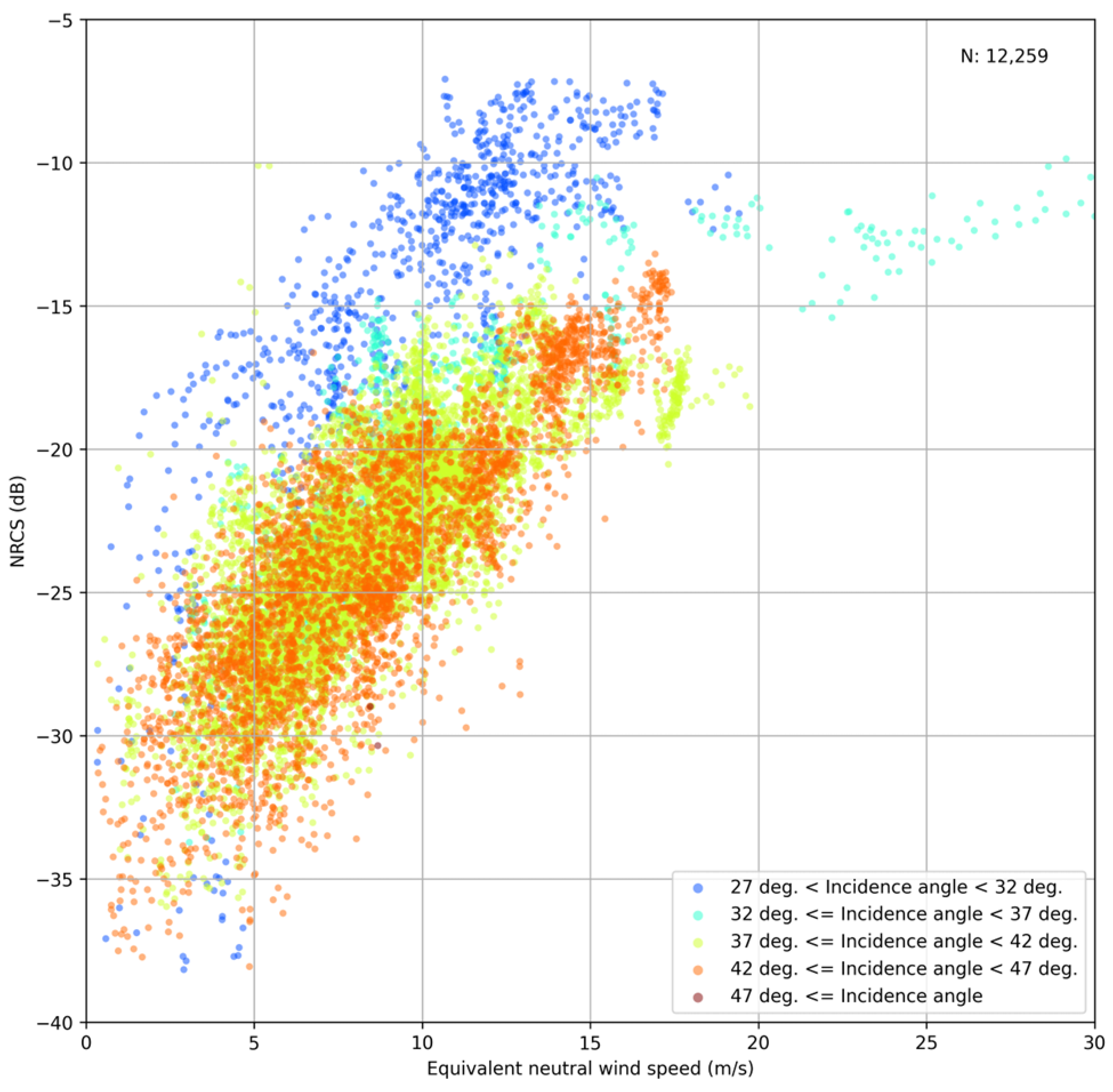
The relationship between the NRCS and incidence angle from ASNARO-2 is shown in Figure 3. The NRCS values decrease with increasing incidence angle. Figure 4 also shows the relationship between the NRCS and the ENW speed from the LFM. The NRCS increases with increasing the ENW speed. These trends are consistent with the Bragg scattering theory. Here, the NRCS values are divided into 1° incidence angle bins from 26 to 47° when determining A 0 . In accordance with previous GMFs and the relationship between the NRCS and the ENW speed (Figure 4), the following equation is employed to represent A 0 as a cubic function,
A 0 = 10 ( a 0 U 3 + a 1 U 2 + a 2 U + a 3 ) / 10
Here, U represents the logarithm of the ENW speed, i.e., l o g 10 u . From Figure 3, it is also found that the variation in NRCS is large even for the same incidence angle bin. To ensure convergence of the calculation, NRCS values that are within 1.6σ (66.3%) from the approximation curves, which were determined based on the relationship between NRCS and ENW for each incidence angle bin, were selected before determining the coefficients. A total of 8128 points were chosen. To determine the coefficients a0, a1, a2, and a3, two different cubic functions are used for each incidence angle bin. One is based on the mean NRCS for each 1 m/s wind speed bin, and the other is based on the mean wind speed for each 1 dB NRCS. These two functions are averaged to make new functions for each incidence angle bin. Figure 5 shows the coefficients a0, a1, a2, and a3 for each incidence angle. Furthermore, each coefficient can be represented as a quadratic or linear function of the incidence angle as follows:
a 0 = c 0 x 2 +   c 1 x + c 2
a 1 = c 3 x 2 +   c 4 x + c 5
a 2 = c 6 x 2 +   c 7 x + c 8
a 3 = c 9 x + c 10
where x = θ 36.5 / 18.25 , and θ is the incidence angle. Using the determined coefficients, the relationship between reproduced A 0 and the NRCS is shown in Figure 6. The bias is 0.17 dB, and the RMSD is 1.41 dB.

3.2. Determination of A 1 and A 2

A 1 and A 2 are iteratively determined based on Equation (3) for each incidence angle bin and wind speed bin. The coefficients for the linear functions of the wind speed, B, C, D, and E are then determined as follows:
A 1 = B   u + C
A 2 = D   u + E
where u is the wind speed. As same as a 0 , a 1 , and a 2 , quadratic functions of the incidence angle, B, C, D, and E are used to produce approximation curves, and the coefficients a 11   a 22 are calculated as follows:
B = c 11 x 2 +   c 12 x + c 13
C = c 14 x 2 +   c 15 x + c 16
D = c 17 x 2 +   c 18 x + c 19
E = c 20 x 2 +   c 21 x + c 22

4. Evaluation of the GMF

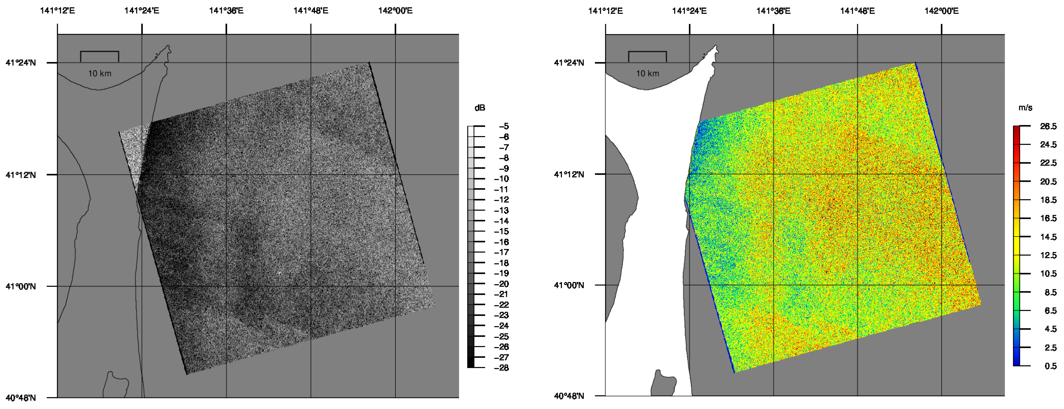
To evaluate the reproducibility of the developed GMF, Figure 7 shows the retrieved wind speeds from ASNARO-2 images with the developed GMF and the ENW speeds obtained from the LFM. All developed formulas and coefficients are summarized in Appendix A. The retrieved wind speed has a bias of −0.10 m/s and an RMSD of 1.37 m/s. The retrieved wind speeds and LFM wind speeds are in good agreement from 3 m/s to 17 m/s. However, the GMF seems to overestimate when the wind speed is lower than 3 m/s and underestimate when the wind speed is higher than 19 m/s. The retrieved wind speed seems to be less accurate when there are a small number of matching points in each wind speed bin (Figure 4). As an example of the wind speed retrieval, Figure 8 shows an NRCS image observed by ASNARO-2 on 12 October 2022 and a wind speed distribution map obtained from the image by the developed GMF with LFM wind direction of 280 degrees. The NRCS is lowest in the waters near the coastline and increases offshore from there. Corresponding to the NRCS image, the wind distribution shows that low wind speeds (<5 m/s) are distributed near the coast and higher (>10 m/s) east of there.
Moreover, the retrieved wind speeds are compared to the in situ wind speeds observed by the KEO buoy (Figure 9). The retrieved wind speed has a bias of 0.03 m/s and an RMSD of 1.68 m/s. The accuracy of these retrieved wind speeds is comparable to previous studies with C-band and X-band SARs.

5. Discussion

This section discusses the prospective improvements of the developed GMF and the outlook for ocean monitoring through SAR images. Figure 10 shows the dependence of the errors in wind speed retrieved with the GMF on the incidence angle. When the incidence angle is more than 44° or less than 28°, the GMF wind speed is significantly lower than the LFM wind speed. In these incidence angles, the number of matching points is small, explaining the low accuracy. As mentioned during the evaluation of GMFs, the small number of matching points greatly affects the accuracy of the GMF.
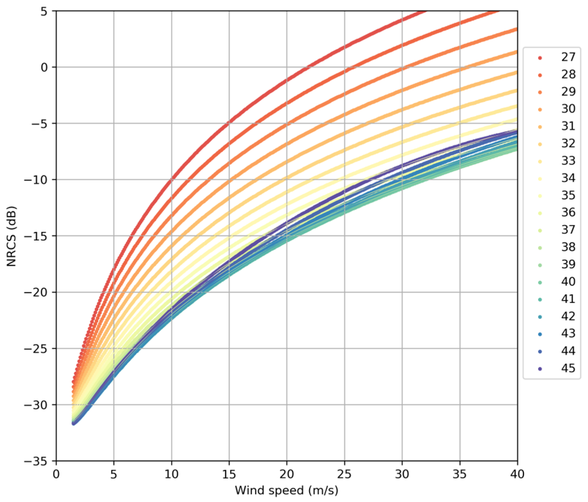
A further point that could be improved is the relationship between the NRCS and the wind speed based on the GMF shown in Figure 11. The NRCS generally decreases with increasing incidence angle. However, for an incidence angle of 45°, the NRCS is higher than at 40° in the developed GMF. This is opposite to the normal relationship between the incidence angle and the NRCS and indicates that the NRCS for the incidence angle of 45° could be overestimated, or the NRCS for the incidence angle of 40° could be underestimated. In Figure 3, the NRCS for an incidence angle of 44° appears higher than that of 36 to 42°. The characteristics of the data used are reflected in the developed GMF. In order to clarify whether the tendency is a radar feature or an error, a series of more continuous observations will be required.
In addition, while this study developed the GMF for ENW, a method using stress-equivalent winds has been proposed in previous studies [26]. As a next step, it would be expected to improve the GMF to consider stress-equivalent winds.
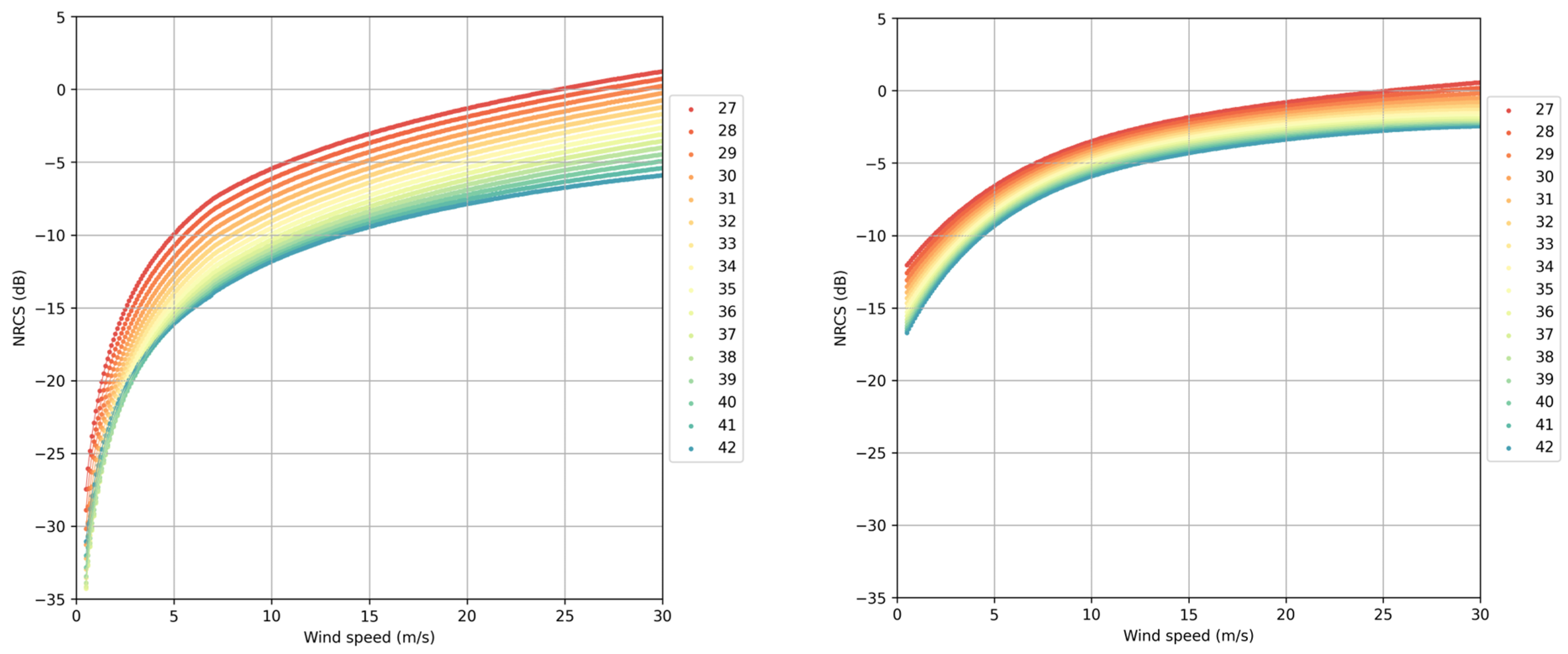
To compare the developed GMF with the existing X-band GMFs, Figure 12 shows the relationship between wind speed and NRCS in XMOD2 for TerraSAR-X and for COSMO-SkyMed. It can be seen that the NRCSs of TerraSAR-X and COSMO-SkyMed differ greatly even for the same wind speed, angle of incidence, and relative wind direction. These characteristics of the NRCS also differ from that with ASNARO-2, as shown in Figure 11. This clearly indicates that the existing X-band GMFs cannot be applied to ASNARO-2. The reason for this difference in NRCS needs to be continued to be investigated, but it can be clearly shown that offshore wind speed is retrieved using the developed GMF from ASNARO-2 images.

6. Conclusions

This study developed a new GMF for the X-band SAR on the ASNARO-2. There are X-band GMFs, but these cannot be applied to ASNARO-2 because the NRCS characteristics of ASANRO-2 are different from those of the existing X-band SARs.
Compared with the LFM wind speeds, wind speeds retrieved by the developed GMF showed reproducibility with a bias of −0.10 m/s and an RMSD of 1.37 m/s. Moreover, it is found that the wind speed has the bias and RMSD were 0.03 and 1.68 m/s, respectively, when compared to the in situ wind speed from the KEO buoy. The results show that ASNASO-2 images can be used to retrieve offshore wind speeds with the same or better accuracy than previous studies. Meanwhile, it was found that the accuracy of wind speed decreased at low and high incidence angles. In addition, inconsistencies in the relationship between incidence angle and NRCS were identified. These issues have room for improvement. Further investigation would be needed to determine how the NRCS characteristics of ASNARO-2 differ from those of other X-band SARs.

Author Contributions

Conceptualization, Y.T.; methodology, Y.T.; validation, Y.T.; formal analysis, Y.T. and S.K.; investigation, Y.T.; resources, Y.T. and S.K.; data curation, Y.T. and S.K.; writing—original draft preparation, Y.T.; writing—review and editing, Y.T.; visualization, Y.T.; supervision, Y.T.; project administration, Y.T.; funding acquisition, Y.T. All authors have read and agreed to the published version of the manuscript.

Funding

This research was funded by the Adaptable and Seamless Technology Transfer Program through Target-driven R&D (A-STEP) from Japan Science and Technology Agency (JST) Grant Number JPMJTR20R7 and Japan Society for the Promotion of Science (JSPS) KAKENHI Grant Number 23K04249.

Institutional Review Board Statement

Not applicable.

Informed Consent Statement

Not applicable.

Data Availability Statement

ASNARO-2 images that support the findings of this study are provided by the Japan EO Satellite Service, Ltd. (JEOSS). LFM is also provided by the Japan Meteorological Agency (JMA). OSTIA SST and KEO buoy data are openly available at the Physical Oceanography Distributed Active Archive Center (PO.DAAC) and the National Oceanic and Atmospheric Administration (NOAA) Pacific Marine Environmental Laboratory (PMEL), respectively.

Acknowledgments

We would like to thank the Japan EO Satellite Service, Ltd. (JEOSS) for their cooperation in providing the ASNARO2 images.

Conflicts of Interest

Shota Kurokawa is an employee of Tokyo Electric Power Services Company, Limited (TEPSCO). The paper reflects the views of the scientists and not the company.

Appendix A

All equations and coefficients of the developed GMF are shown as follows.
σ 0 = A 0 1 + A 1 cos φ + A 2 cos 2 φ
A 0 = 10 ( a 0 U 3 + a 1 U 2 + a 2 U + a 3 ) / 10
U = l o g 10 u       ( u > 1 )
A 1 = B   u + C
A 2 = D   u + E
a 0 = c 0 x 2 +   c 1 x + c 2
a 1 = c 3 x 2 +   c 4 x + c 5
a 2 = c 6 x 2 +   c 7 x + c 8
a 3 = c 9 x + c 10
B = c 11 x 2 +   c 12 x + c 13
C = c 14 x 2 +   c 15 x + c 16
D = c 17 x 2 +   c 18 x + c 19
E = c 20 x 2 +   c 21 x + c 22
x = θ 36.5 / 18.25
Table A1. Coefficients of GMF for ASNARO-2.
A0a0c09.11336
c16.49630
c2−2.77146
a1c3−12.73693
c4−7.61105
c515.10509
a2c625.45840
c7−6.41516
c8−2.33088
a3c9−3.85802
c10−30.61375
A1Bc11−0.10040
c12−0.00201
c130.02240
Cc140.65642
c150.11324
c16−0.20075
A2Dc170.02618
c180.05286
c190.01195
Ec20−0.02781
c21−0.67547
c220.03487

References

  1. Stoffelen, A.; Anderson, D. Scatterometer Data Interpretation: Estimation and Validation of the Tranfer Function CMOD4. J. Geophys. Res. 1997, 102, 5767–5780. [Google Scholar] [CrossRef]
  2. Quilfen, Y.; Chapron, B.; Elfouhaily, T.; Katsaros, K.; Tournadre, J. Observation of Tropical Cyclones by High-Resolution Scatterometry. J. Geophys. Res. 1998, 103, 7767–7786. [Google Scholar] [CrossRef]
  3. Hersbach, H.; Stoffelen, A.; Haan, S. An Improved C-Band Scatterometer Ocean Geophysical Model Function: CMOD5. J. Geophys. Res. 2007, 112, C03006. [Google Scholar] [CrossRef]
  4. Hersbach, H. Comparison of C-Band Scatterometer CMOD5.N Equivalent Neutral Winds with ECMWF. J. Atmos. Ocean. Technol. 2010, 27, 721–736. [Google Scholar] [CrossRef]
  5. Stoffelen, A.; Verspeek, J.A.; Vogelzang, J.; Verhoef, A. The CMOD7 Geophysical Model Function for ASCAT and ERS Wind Retrievals. IEEE J. Sel. Top. Appl. Earth Obs. Remote Sens. 2017, 10, 2123–2134. [Google Scholar] [CrossRef]
  6. Lehner, S.; Horstmann, J.; Koch, W.; Rosenthal, W. Mesoscale Wind Measurements Using Recalibrated ERS SAR Images. J. Geophys. Res. 1998, 103, 7847–7856. [Google Scholar] [CrossRef]
  7. Christiansen, M.B.; Koch, W.; Horstmann, J.; Bayhasager, C.; Nielsen, M. Wind Resource Assessment from C-Band SAR. Remote Sens. Environ. 2006, 105, 68–81. [Google Scholar] [CrossRef]
  8. Hasager, C.B.; Badger, M.; Peña, A.; Larsén, X.G.; Bingöl, F. SAR-Based Wind Resource Statistics in the Baltic Sea. Remote Sens. 2011, 3, 117–144. [Google Scholar] [CrossRef]
  9. Takeyama, Y.; Ohsawa, T.; Kozai, K.; Hasager, C.B.; Badger, M. Comparison of Geophysical Model Functions for SAR Wind Speed Retrieval in Japanese Coastal Waters. Remote Sens. 2013, 5, 1956–1973. [Google Scholar] [CrossRef]
  10. Takeyama, Y.; Ohsawa, T.; Yamashita, T.; Kozai, K.; Muto, Y.; Baba, Y.; Kawaguchi, K. Estimation of Offshore Wind Resources in Coastal Waters off Shirahama Using ENVISAT ASAR Images. Remote Sens. 2013, 5, 2883–2897. [Google Scholar] [CrossRef]
  11. Takeyama, Y.; Ohsawa, T.; Kozai, K.; Hasager, C.B.; Badger, M. Effectiveness of WRF Wind Direction for Retrieving Coastal Sea Surface Wind from Synthetic Aperture Radar. Wind Energy 2013, 16, 865–878. [Google Scholar] [CrossRef]
  12. Chang, R.; Zhu, R.; Badger, M.; Hasager, C.B.; Xing, X.; Jiang, Y. Offshore Wind Resources Assessment from Multiple Satellite Data and WRF Modeling over South China Sea. Remote Sens. 2015, 7, 467–487. [Google Scholar] [CrossRef]
  13. Hasager, C.B.; Mouche, A.; Badger, M.; Bingöl, F.; Karagali, I.; Driesenaar, T.; Stoffelen, A.; Peña, A.; Longépé, N. Offshore Wind Climatology Based on Synergetic Use of Envisat ASAR, ASCAT and QuikSCAT. Remote Sens. Environ. 2015, 156, 247–263. [Google Scholar] [CrossRef]
  14. Ahsbahs, T.; Badger, M.; Karagali, I.; Larsén, X.G. Validation of Sentinel-1A SAR Coastal Wind Speeds against Scanning LiDAR. Remote Sens. 2017, 9, 552. [Google Scholar] [CrossRef]
  15. Kim, D.; Moon, W.M. Estimation of Sea Surface Wind Vector Using RADARSAT Data. Remote Sens. Environ. 2002, 80, 55–64. [Google Scholar] [CrossRef]
  16. Mouche, A.; Chapron, B. Global C-Band Envisat, RADARSAT-2 and Sentinel-1 SAR Measurements in Copolarization and Cross-Polarization. Nature 2015, 120, 7195–7207. [Google Scholar] [CrossRef]
  17. Zhang, B.; Mouche, A.; Lu, Y.; Perrie, W.; Zhang, G.; Wang, H. A Geophysical Model Function for Wind Speed Retrieval from C-Band HH-Polarized Synthetic Aperture Radar. IEEE Geosci. Remote Sens. Lett. 2019, 16, 1521–1525. [Google Scholar] [CrossRef]
  18. Lu, Y.; Zhang, B.; Perrie, W.; Mouche, A.A.; Li, X.; Wang, H. A C-Band Geophysical Model Function for Determining Coastal Wind Speed Using Synthetic Aperture Radar. IEEE J. Sel. Top. Appl. Earth Obs. Remote Sens. 2018, 11, 2417–2428. [Google Scholar] [CrossRef]
  19. Qin, T.; Jia, T.; Feng, Q.; Li, X. Sea Surface Wind Speed Retrieval from Sentinel-1 HH Polarization Data Using Conventional and Neural Network Methods. Acta Oceanol. Sin. 2021, 40, 13–21. [Google Scholar] [CrossRef]
  20. Isoguchi, O.; Shimada, M. An L-Band Ocean Geophysical Model Function Derived from PALSAR. IEEE Trans. Geosci. Remote Sens. 2009, 47, 1925–1936. [Google Scholar] [CrossRef]
  21. Ren, Y.; Lehner, S.; He, M. Study on X-Band Polarization Ratio with TerraSAR-X Images. In Proceedings of the SPIE—Remote Sensing and Modeling of the Atmosphere, Oceans, and Interactions III, Incheon, Republic of Korea, 13–14 October 2010; Volume 7856. [Google Scholar] [CrossRef]
  22. Li, X.M.; Lehner, S. Algorithm for Sea Surface Wind Retrieval from TerraSAR-X and TanDEM-X Data. IEEE Trans. Geosci. Remote Sens. 2014, 52, 2928–2939. [Google Scholar] [CrossRef]
  23. Nirchio, F.; Venafra, S. XMOD2—An Improved Geophysical Model Function to Retrieve Sea Surface Wind Fields from Cosmo-SkyMed X-Band Data. Eur. J. Remote Sens. 2013, 46, 583–595. [Google Scholar] [CrossRef]
  24. Liu, W.T.; Tang, W. Equivalent Neutral Wind; JPL Publication 96-17; National Aeronautics and Space Administration, Jet Propulsion Laboratory: Pasadena, CA, USA; California Institute of Technology California: Pasadena, CA, USA, 1996. [Google Scholar]
  25. Good, S.; Fiedler, E.; Mao, C.; Martin, M.J.; Maycock, A.; Reid, R.; Roberts-Jones, J.; Searle, T.; Waters, J.; While, J.; et al. The Current Configuration of the OSTIA System for Operational Production of Foundation Sea Surface Temperature and Ice Concentration Analyses. Remote Sens. 2020, 12, 720. [Google Scholar] [CrossRef]
  26. De Kloe, J.; Stoffelen, A.; Verhoef, A. Improved Use of Scatterometer Measurements by Using Stress-Equivalent Reference Winds. IEEE J. Sel. Top. Appl. Earth Obs. Remote Sens. 2017, 10, 2340–2347. [Google Scholar] [CrossRef]
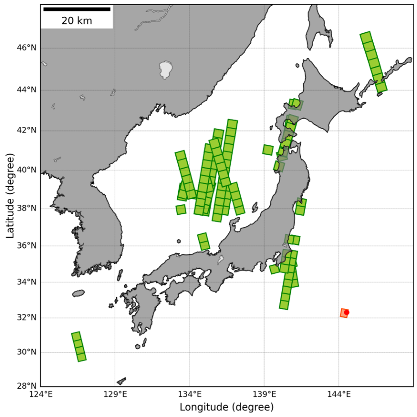
Figure 1. ASNARO-2 observation areas around Japan and the location of the KEO buoy shown as a red circle. Areas used for the GFM development are surrounded by green squares, and areas used for a validation are surrounded by red squares.
Atmosphere 15 00686 g001
Figure 2. Number of matching points in each relative wind direction bin.
Atmosphere 15 00686 g002
Figure 3. Relationship between NRCS and incidence angle from ASNARO-2.
Atmosphere 15 00686 g003
Figure 4. Relationship between NRCS from ASNARO-2 and the ENW speed from the LFM.
Atmosphere 15 00686 g004
Figure 5. Dependence of a 0 , a 1 , a 2 , and a 3 on incidence angle.
Atmosphere 15 00686 g005
Figure 6. Relationship between reproduced A 0 and NRCS.
Atmosphere 15 00686 g006
Figure 7. Relations between retrieved wind speeds from ASNARO-2 images with the developed GMF and ENW speeds from the LFM. Red circles represent averages of wind speeds every 2 m/s.
Atmosphere 15 00686 g007
Figure 8. An example of an NRCS image (left) and wind speed (right) retrieved with the developed GMF from ASNARO-2 images observed on 12 October 2022.
Atmosphere 15 00686 g008
Figure 9. The relationship between retrieved wind speeds from ASNARO-2 images with the developed GMF and in situ speeds from the KEO buoy.
Atmosphere 15 00686 g009
Figure 10. Relationship between errors of the retrieved wind speeds from ASNARO-2 images and incidence angle. Red circles represent averages of incidence angles every 2 degrees.
Atmosphere 15 00686 g010
Figure 11. Relationship between NRCS and wind speed for each incidence angle from 27 to 45 degrees in the developed GMF when the relative wind direction is 0 degrees.
Atmosphere 15 00686 g011
Figure 12. Relationships between NRCS and wind speed for each incidence angle from 27 to 45 degrees in GMFs for XMOD2 with TerraSAR-X [22] (left) and improved XMOD2 for COSMO-SkyMed [23] (right) when the relative wind direction is 0 degrees.
Atmosphere 15 00686 g012
Table 1. Specifications of ASNARO-2.
SatelliteAdvanced Satellite with New System Architecture for Observation-2 (ASNARO-2)
OperationNEC corporation
Launch date17 January 2018
OrbitSun-synchronous circular orbit
Altitude817 km
Inclination98.7°
Local time of descending node9:30
Orbital period107.1 min
Ground track repeat cycle29 days
Disclaimer/Publisher’s Note: The statements, opinions and data contained in all publications are solely those of the individual author(s) and contributor(s) and not of MDPI and/or the editor(s). MDPI and/or the editor(s) disclaim responsibility for any injury to people or property resulting from any ideas, methods, instructions or products referred to in the content.