Abstract
Selecting appropriate climate change scenarios is crucial, as it influences the outcomes of climate change impact studies. Several storylines could be used to investigate the sensitivity of water resource schemes to weather variability and improve policymakers’ adaptation strategies. This study proposes a comprehensive and generic methodology for assessing the future climate change impact on semi-arid and arid zones at the basin scale by comparing delta perturbation scenarios to the outcomes of seven collections of GCMs (general circulation models). The findings indicate that the two scenarios predicted nearly identical declines in average reservoir discharges over a monthly timescale. Consequently, their maximum values are almost similar. The projected decrease in the streamflow for the period 2080–2099 is approximately 48%—the same as the ratio from the delta perturbation scenario of Future16 (a 30% precipitation decrease and a 30% potential evapotranspiration increase). Furthermore, delta perturbation scenarios allow the impacts of model sensitivity to climate change to be clearly identified in relation to GCM scenarios. Delta perturbation scenarios allow for an extensive collection of possible climate changes at the regional scale. In addition, delta perturbation scenarios are simpler to create and use; therefore, they might complement GCM scenarios.
1. Introduction
1.1. Background
Climate change is currently affecting different biological and physical systems [1]. Several general circulation models (GCMs) predict an increase in the number and frequency of extreme climate events [1], which could significantly impact global water resources [2,3]. Rainfall–runoff models are commonly used to investigate the effects of climate change on regions, using weather data from GCMs as inputs [2]. However, the inherent simplifications in these climatic models limit their ability to simulate the Earth’s weather system, resulting in model outputs with a wide range of biases related to the observed climate [4]. Thus, improving GCM performance through multiple preprocessing techniques is crucial., As part of these improvements, downscaling processes like statistical methods and regional climate models (RCMs) have begun.
Precipitation is considered one of the most critical variables in studies on the effects of climate change. However, accurately assessing its variations is challenging due to its spatiotemporal variability, particularly on a daily timescale. Mohammed and Scholz [4] argue that obtaining reliable evaluations of average or daily future precipitation values based on model simulations alone is unlikely. Two well-known techniques for daily precipitation modification are the delta change and bias correction. The former technique measures the climate based on observed simulated changes; the latter derives projections by changing future period simulations based on model biases on the observed weather data.
RCMs are only available for a limited number of areas, and for many practical applications, such as regional hydrology, their outcomes are excessively coarse and computationally demanded. Accordingly, statistical methods have been proposed. Statistical methods incorporate predictands (local-scale variables) with predictors (GCMs or RCMs, large-scale variables) on a regional or basin scale. These measures are relatively simple.
Regression function (transfer), weather typing, and weather generator (WG) are the three main classes of statistical downscaling methods [5,6]. The transfer function method shapes the numerical relationships between predictors and predictands. Regression function methods are relatively easy to apply; nevertheless, the central disadvantage is the absence of a stable connection among large-scale and local-scale variables. The second class encompasses local-scale variables, which relate to various modules of global distribution [5,6]. The main gain is that local-scale variables strongly connect to global circulation. Yet, their dependability is founded on a relationship between predictors and local weather. Overall, there is no clear relationship between large-scale circulation and daily precipitation. The weather generator method depends on the disturbance of its variables and their association with the differences computed by climate simulations [7]. The most important benefit of a weather generator is its ability to generate collections of climate storylines to investigate the effects of extraordinary climatic phenomena and study normality inconsistency. Consequently, the current study employed LARS-WG 7. The WG is named after the place where it was developed in its present form. The LARS-WG7 has been tested in various locations and has demonstrated its capability to realistically simulate rainfall extremes [8].
Many researchers have assessed climate change’s impact on hydro-climatic characteristics at a regional scale [9,10,11,12,13,14]. However, they only studied the effects of climate change based on GCMs that have been downscaled to the local scale using either statistical or regional downscaling methods, without considering other climatic scenarios, such as synthetic or analog. Additionally, researchers such as Chen et al. [15] have stated that the main sources of uncertainty involved in climate change studies are related to GCMs, greenhouse gas emission (GHG) scenarios, and uncertainties regarding the downscaling process. Consequently, to demonstrate such uncertainties and difficulties, previous researchers (e.g., [2,6,16]) used delta perturbation (DP) (change factor) theories. Although Mohammed and Scholz [2] discussed the impact of climate change on water resource management at a local scale in semi-arid and arid zones, their analysis only depended on weather data from DP scenarios without considering the GCM climatic scenario, which is considered in this study. Furthermore, although Mohammed and Scholz [17] discussed the flow alteration in the LZRB, they did not consider the impact of climate change on the hydro-climatic aspects of the region, such as the relationships between the reservoir capacity, yield, and reliability, which are discussed in the present study. Therefore, to fill this gap, the objective of this study is to assess and liken the outcomes of DP and GCM scenarios to answer the following research questions: “Which of these two scenarios performs better in predicting basin hydro-climatic variables?” and “In the climate change assessment, what are the similarities and/or differences between the DP and GCM scenarios?” These issues are addressed because almost all preceding research that dealt with climate change evaluations tended to rely solely on a single scenario (typically the GCMs). Apart from the previous point, this study outlines work that should be considered as novel.
1.2. Aim, Objectives, and Originality
The current study seeks to assess and evaluate the outcomes of GCMs and DP scenarios—which are commonly applied climatic scenarios—to investigate how close or dissimilar the two scenarios are from each other in their ability to model streamflow and reservoir performances. Since the DP approach allows for a wide range of climate change scenarios at the basin scale and makes them simpler to form and utilize, it is strongly advised that this study be reconducted using the combined outcomes of the GCM and DP climate change scenarios. Various scenarios will be utilized to identify the sensitivity of water resource management to climate change and to support water resource managers in adapting to these changes. Based on earlier studies, this work might be considered the first work to address the following questions: Which of these two scenarios more accurately predicts basin hydro-climatic factors? In assessing climate change, what are the potential similarities and/or differences between GCM and DP scenarios? These are interesting research questions, as almost all earlier studies generally depended on a single climate change storyline (usually GCMs). The proposed methodology for assessing the possible effects of climate change on water resource management is shown in Figure 1.
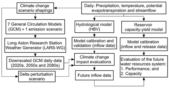
Figure 1.
Proposed novel modeling approach for evaluating the probable climate change impact on the water resource system. Note: HBV is the Hydrologiska Byråns Vattenbalansavdelning rainfall–runoff model.
The primary objectives are to:
- Verify the LARS-WG7 ability to model climate data in a semi-arid climatic zone by using historical metrological data;
- Forecast the potential variation in the meteorological variables downscaled by LARS-WG based on AR6 (the sixth assessment report) of IPCC (the Intergovernmental Panel on Climate Change), under SRA6 (the Special Report on Emission Scenarios) [18] generated by seven GCMs;
- Assess the anticipated impact of climate change on the hydrological parameters of the catchment: RDIst (the standardized reconnaissance drought index), SDI (the streamflow drought index), and OPOF (the reservoir operational probability of failure, %); and
- Identify relationships that integrate reservoir capacity, yield, and reliability. Accordingly, this study could be regarded as comparative basin research through the impact of climate change on the hydro-climatic properties, drought indices, and reservoir performance.
2. Materials and Methods
2.1. Information Collection and Analysis
The daily climatic parameters of ten meteorological sites spread across the representative basin (Figure 2), with elevations ranging from 319 to 1536 m above sea level (m a.s.l.) (Table 1), existed from 1979/1980 to 2012/2013. The collected data include daily discharges for the Dokan hydrological site (longitude 44°58′00″ E and latitude 35°53′00″ N) from over 35 years. This part of the study covers approximately 14,924 km2. The data were provided by the Iraqi Ministry of Agriculture and Water Resources in Kurdistan.
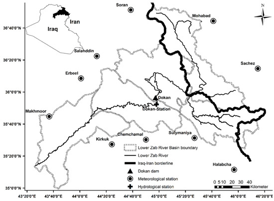
Figure 2.
The basin location example included the hydro-climatic gauging station sites.

Table 1.
Meteorological station addresses in the Lower Zab River Basin.
ArcGIS 10.8 was used to project hydro-climatic station locations, calculate basin average precipitation, and define basins. Table 1 provides a summary of station locations. The Theissen Network method (weighing mean) is used to determine the precipitation’s spatial distribution. For a more in-depth explanation of the weighting mean method, researchers can refer to previous studies, such as [3]. The Statistical Package for Social Sciences (SPSS) 23 [19] was used to analyze hydro-climatic data trends and fill gaps. The potential evapotranspiration (mm) parameter was determined using the Food and Agriculture Organization Penman–Monteith standard method [20] and the reference evapotranspiration ETo (mm) calculator version 3.2 [21].
2.2. Symbolic Regional Study Example
The Lower Zab River (between latitudes 36°50′ N and 35°20′ N and longitudes 43°25′ E and 45°50′ E) is one of the mainly significant branches of the Tigris River [2,22]; Figure 1. The river is situated nearly 220 km north of Baghdad, the capital city [2,22,23]. The corresponding catchment is approximately 19,254 km2 [24].
The Lower Zab River Basin (LZRB) covers a variety of rather large drainage areas with an extensive variety of weather and hydrological conditions. The upper and lower parts of the LZRB development vary generally, which presents a significantly greater variety of doubts about climate change’s effect on the accessibility of water resources. Due to approximately 80% precipitation reduction, the LZRB experienced severe drought during the 2007/2008 hydrological year [22,24]. The extensive drought conditions caused a catastrophic effect on crop production and the lives of the people in the region.
2.3. Climatic Drought Identification
The reconnaissance drought index (RDI) has been applied to identify meteorological drought within the study basin. The RDI index could be expressed as RDIαk (initial/alpha), RDIn (normalized), and RDIst (standardized) types. The standardized form is commonly applied to assess drought severity, although the alpha formula is used as an aridity indicator. RDIαk is primarily based on the collected potential evapotranspiration and precipitation concepts [2,25].
A positive RDIst number indicates a wet period. However, a negative number indicates a dry period relative to the area’s normal conditions. Drought severity increases when RDIst numbers are low. Drought severity is determined by the boundary RDIst value: extremely dry (≤−2.00), severely dry (−1.5 to −1.99), moderately dry (−1 to −1.49), near normal (0.00 to −0.99), normal (0.99 to 0.00), moderately wet (1.49 to 1.00), very wet (1.99 to 1.5), and extremely wet (≥2.00) [16,24,26].
However, to identify hydrological drought, this study applies the stream drought index (SDI), which is based on the discharge gathered capacities S_(i,k) for each duration k of the ith hydraulic year, as shown in Equation (1):
where Mk denotes the cumulative mean of streamflow storage; and SDk denotes the cumulative standard deviation of streamflow storage for the reference period k, as they are long-term estimates.
Streamflow in most small basins has a skewed probability distribution. Gamma distribution functions can estimate this. Then, this distribution is transformed into a normal distribution. The definition of the SDI index using the two-parameter log-normal distribution is provided in Equation (2).
Hence, using Equation (3), the cumulative natural logarithms of streamflow with mean and standard deviations SDik may be computed.
2.4. Reservoir Capacity-Yield Model and Performance Indices
The Hydrologiska Byråns Vattenbalansavdelning (HBV) rainfall–runoff model was used to assess the performance of the reservoir capacity yield (RCY). The model requires a small amount of input data. The model only needs daily precipitation, temperature, and monthly evapotranspiration. The model calibration period was considered from 1988 to 1999, while the model validation period was considered from 1979 to 1986. The HBV simulates daily streamflow based on the corresponding rainfall, temperature, and potential evapotranspiration data contributions. Temperature is used for computing the accumulation of snow.
The RCY model was accomplished using Equation (1) from McMahon and Adeloye [26]:
where St+1 and St are the reservoir storage volumes at the end and beginning of a duration t, in this order; Qt is the inflow during the period t; Dt is the real water yield in time t; ΔEt is the net evaporation from the reservoir during time t; Lt comprises further losses; and C is the active reservoir capacity.
Many pre-processing processes were carried out for the inflow data to build the reservoir capacity, yield, and reliability correlations. Initially, the elevation, area, and capacity correlations for rainfall and evaporation were constructed to estimate the volume properties of these weather variables. When running simulations, the reservoir, So, is normally understood to be full [27], and the downstream requirement is commonly seen as a specific fraction of the average inflow. The OPOF can be calculated as follows: (a) assume the lake is filled at the beginning (So = C); (b) use Equation (1) month by month for the past discharges; (c) plot St+1 against time on a monthly timescale; and (d) calculate the OPOF by applying Equation (3). When applying RCY analysis, the reservoir vulnerability is calculated, disregarding the limitation on Equation (1), and selecting the maximum negative number for St+1 in the investigation; however, the resilience is based on the maximum consecutive number of empty months in the assessment [28]. The following performance indicators are used to evaluate the simulations [9,27]: (1) the time-based reservoir reliability Re is characterized as the ratio of the total duration under assessment, during which an impoundment provides the water demand according to Equation (2).
where Re represents reservoir reliability (%) and OPOF represents the operational likelihood of failure (%), which is characterized as the ratio of time the reservoir is empty to the total assessment time (Equation (3)).
where Ne denotes the period when the reservoir is unfilled, and N denotes the total time linked to the streamflow time series. The OPOF is not limited. However, 5% is seen as an acceptable limitation [26].
The resilience, φ, is characterized as the reservoir’s ability to recover from the failure, as shown in Equation (4) and previously discussed by many researchers [5,29]. Moy et al. [28] defined resilience as the maximum number of consecutive time units of deficiency occurring before recovery.
where Yt refers to the continuous deficiency meter value, Yt = 1, assuming that there is a deficiency in the period t, Yt = 0, and t = 1, 2,…, N, which is the overall time unit number in the time serious representing the streamflow data sequence of failure times.
The vulnerability, ν, is a measure to calculate the significance of failure. Mathematically, it is calculated by applying Equation (5) as shown by Fowler et al. [29] and Park and Kim [5].
where ν is the vulnerability, and Dft is the deficit at time t, as discussed previously [9,27].
2.5. Delta Perturbation Climatic Scenario
In the delta perturbation (DP) climatic techniques, the climatic variables are perturbed incrementally by random values. For example, +1 and +4 °C changes in air temperature can be linked with −4 or −6% (or 0 changed) precipitation changes to build an incremental scenario [1]. Equation (9) may be applied to this scenario.
where AMVt refers to the expected meteorological variable (mm), OMVt is the observed meteorological variable (mm), RA refers to the added or subtracted ratio (%), and t is the time step.
Perturbation scenarios are often based on the assumption of a consistent annual change in climatic variables. These scenarios are user-friendly, offer data on a wide range of potential differences, and can be easily and reliably applied to different areas. They frequently represent realistic sets of physically reasonable variations, especially when constant changes are applied over a large area or when assumed parameter changes are not physically consistent with one another. Their primary application is in exploring system sensitivity. Many recent climate change studies have utilized this type of scenario (e.g., [6,16,17,30]). In this study, climatic scenarios were developed by adjusting historical values of potential evapotranspiration and precipitation by 2% within ranges of 0 to +30% and 0 to −40%, respectively. As a result, all potential combinations within the considered ranges (approximately 336 scenarios formulated) of precipitation and potential evapotranspiration variations were taken into account. These scenarios encompass all climate change projections for the studied region. Although the DP technique does not involve alterations in the distribution likelihood concerning climatic characteristics and seasonal changes, it is still an appropriate technique for detecting tipping points in general [17].
2.6. Long Ashton Research Station Weather Generator Model
The Long Ashton Research Station Weather Generator (LARS-WG) is a widely recognized software tool for simulating weather conditions and it is commonly used in climate impact research [31]. LARS-WG can effectively model meteorological parameters for current and potential weather conditions at a relatively low cost. The latest version, LARS-WG7, includes climate scenarios based on the CMIP6 ensemble [18], a comprehensive dataset of future climate projections generated by leading modeling groups worldwide. By using multi-model ensembles, researchers can explore the uncertainty in climate predictions stemming from differences in global climate model design and variations in initial conditions or model parameters. This version also enhances the simulation of extreme weather events such as heavy daily precipitation, prolonged dry spells, and heat waves. LARS-WG has undergone extensive validation in diverse climates across the globe.
The model utilizes daily data from a specific site to analyze climate parameters like precipitation (mm), maximum and minimum temperature (°C), and solar radiation (MJ/m2/day). It estimates probability distribution parameters for these weather variables and their relationships, allowing for the creation of an artificial climate time series of a random length. By perturbing distribution variables based on estimated climate changes from global or local climate models, daily climatic scenarios can be generated and used for impact evaluation. The model has shown strong performance in replicating various climate data sets, including extreme weather events [31].
The simulation of rainfall occurrence is based on the distribution of the length of a continuous series of wet and dry days, with the distributions of maximum and minimum temperatures dependent on the current wet or dry series [30]. LARS-WG7 utilizes a semi-empirical distribution, specifically the cumulative probability distribution function, to predict distributions for dry and wet periods, daily extreme temperatures, precipitation, solar radiation, and potential evapotranspiration. Equation (7) is used to calculate the probability pi for each weather parameter v.
with fixed values p0 = 0 and pn =1 corresponding to v0 = min{vobs} and vn= min{vobs} for each climatic variable.
To accurately estimate the maximum values of a weather parameter, certain values of pi near 0 represent very low numbers, while values near 1 represent very high ones; the remaining pi values are evenly distributed on the likelihood scale. For the precipitation scenario, three values close to 1 are used: pn−1= 0.999, pn−2 = 0.995, and pn−3 = 0.985, allowing for a better estimation of events with very high day-to-day rainfall and low probability, such as rainfall during hurricanes.
The LARS-WG7 model utilizes 23 SED, offering a more precise depiction of the observed distribution compared to the previous model that relied on 10 SED [15]. Furthermore, the updated model enhances the simulation of extreme air temperatures for dry and wet days by incorporating a semi-empirical distribution, as well as monthly calculations for auto- and cross-correlations. For a comprehensive understanding of the LARS-WG7 method, please refer to Semenov and Stratonovitch [31].
The artificial climate generation technique consists of the following key steps.
- The site analysis function is used to calibrate models by analyzing recorded meteorological data and estimating statistical properties. The obtained results are saved as two parameter files.
- The QTest function is used for model validation, which examines the statistical properties of the recorded and artificial meteorological data to see if there are any statistically significant variations; and
- The generator function produces fictitious meteorological data. The parameter files derived during the model calibration are used to produce artificial meteorological data that have similar statistical properties to the recorded data but are different on a day-to-day basis. Artificial data equivalent to a specific climate change scenario may also be produced by applying global climate model-derived changes in temperature, precipitation, and solar radiation to the LARS-WG parameter files. Furthermore, a daily local climate scenario is generated by changing distribution variables at a location based on the anticipated weather variations resulting from global or local weather simulations. The generated climatic scenarios can then be utilized in combination with a procedure found to influence models for impact evaluation.
To create weather scenarios for a specific period in the future and a certain emission scenario, the LARS-WG baseline parameters estimated from the past climatic data are modified by the expected delta differences for the duration, and the emissions are anticipated by a GCM for every climate factor for the system linked to the site. Ensemble GCMs offer a more accurate depiction of possible climate changes by accounting for uncertainties associated with natural variability, socioeconomic advancements, and model inconsistencies. For climate impact research, however, the increasing number of GCMs presents computational difficulties. To address these issues, a range of model reduction strategies are being developed that improve efficiency and usability while maintaining crucial GCM ensemble properties [32]. For this research, regional-scale climate scenarios are based on the CMIP6 states modeled by seven GCM groups (Table 2) and imitated by LARS-WG, to forecast future temperature and precipitation changes in the Lower Zab River Basin from 2011 to 2030, 2046 to 2065, and 2080 to 2099.

Table 2.
The Long Ashton Research Station Weather Generator (LARS-WG) incorporates selected global climate models from the IPCC’s sixth assessment report (AR6) [18].
3. Results
3.1. LARS-WG Calibration and Validation
The LARS-WG7 calibration and validation process utilized daily weather data from 1980–2010 at ten meteorological stations. Various statistical tests and graphical comparisons were used to assess the model, including the Kolmogorov–Smirnov (K-S) method to analyze the equivalence of wet or dry series periodic distributions (WD Series), daily rainfall distributions (RainD), and daily minimum (TminD) and maximum (TmaxD) temperature distributions. The K-S method generated a p-value to evaluate whether the observed and downscaled data could have come from the same distribution. A low p-value coupled with a high K-S value indicates that the generated climate differs from the recorded climate and should be rejected. While the common significance level is a p-value of 0.05, a 0.01 p-value has been suggested as an acceptable limit of significance. Variations between recorded and simulated data can be attributed to factors such as model smoothing, flaws in recorded data, random variability, and unusual climate phenomena.
Evaluating wet and dry spell patterns throughout the seasons, as well as the distribution of daily rainfall each month, is crucial when using downscaling simulation results in impact research. In this context, Table 3 and Table 4 present the K-S test results from the validation phase, which indicate the model’s performance in replicating the recorded seasonal data and monthly rainfall distribution. It is noteworthy that LARS-WG7 demonstrated a high level of accuracy in capturing the seasonal distribution, with the fit of wet and dry spell series ranging from perfect to very good (1 ≥ p-value ≥ 0.7) as shown in Table 3. Additionally, the model’s performance in replicating the distribution of wet and dry spells during the spring season “MAM” (March, April, and May) was rated as very good to perfect.

Table 3.
The Long Ashton Research Station Weather Generator (LARS-WG7) validation results, including the Kolmogorov–Smirnov (K-S) test, cover the distributions for wet and dry season series distributions during the baseline period of 1980–2010.

Table 4.
The Long Ashton Research Station Weather Generator (LARS-WG7) validation results, including the Kolmogorov–Smirnov (K-S) test for daily rain distributions during the baseline period of 1980–2010.
However, during the summer season, “JJA” (June, July, and August), the model’s performance in replicating the distribution of wet spells was slightly lower. This can be attributed to the dry nature of the JJA season, resulting in minimal observed rainfall, therefore limiting the model’s ability to accurately replicate wet spell distribution. Overall, while LARS-WG7 performed well in capturing the dry spell distribution during the winter season, “DJF” (December, January, and February), it faced challenges in replicating the wet spell distribution during the dry summer season.
Furthermore, Figure 3 shows that the LARS-WG7 performance in modeling the distribution of daily rainfall for all months ranged from “very good” to “perfect” (except in the summer), which can be attributed to the same factors responsible for the poor performance in simulating the seasonal distributions that have been given previously.
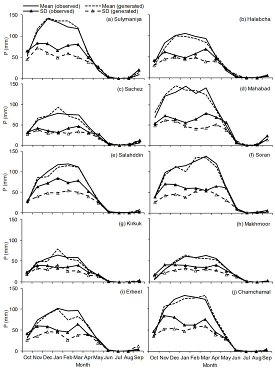
Figure 3.
Comparison between observed monthly (mean and standard deviation (SD)) precipitation (P) and the corresponding values generated by LARS-WG7 at each meteorological station within the studied basin for the period 1980–2010.
To increase the confidence level of the prediction capability of the model, comparisons between the monthly averages and corresponding standard deviations (SD) of the recorded and generated precipitation have been implemented for all stations. Figure 3 shows that there are good matches between the modeled and recorded precipitation for the whole station. Nevertheless, the SD performance is not as good as that of the average, but the outcomes can be considered reasonably good because it is challenging to model SD well with most downscaling tools. Moreover, Figure 4 indicates that LARS-WG7 simulated the monthly average values of Tmax and Tmin very well, which verifies that this version of LARS-WG effectively predicts extreme temperatures.
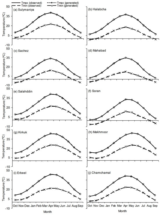
Figure 4.
Comparison between the observed mean monthly (maximum (Tmin) and minimum (Tmax) temperatures and the corresponding values generated by LARS-WG7 at each meteorological station within the studied basin for the period 1980–2010.
From the above, it can be seen that the model performs well in producing daily precipitation, Tmin, and Tmax for most stations. It follows that the model can then be utilized to predict daily weather values for the ten stations during the periods 2011–2030, 2046–2065, and 2080–2099, depending on the seven GCM scenario ensembles.
3.2. Climate Change Impact
3.2.1. Meteorological Variables
The mean meteorological variable values produced by seven GCM assemblies using the SRA2 production storyline for the potential intervals (2011–2030, 2046–2065, and 2080–2099) are shown in Figure 5. In general, both Tmin and Tmax exhibit an increasing tendency, whereas precipitation demonstrates a decreasing tendency. The predicted Tmin shows maximum increases of 0.54, 3.02, and 4.36 °C during the 2011–2030, 2046–2065, and 2080–2099 time intervals, respectively (Figure 5a). Additionally, Tmax is estimated to increase with the greatest figures of 0.56, 2.49, and 4.70 °C for the three considered time intervals, respectively (Figure 5b). Precipitation totals decline by 6.32, 17.33, and 340.18 mm, respectively (Figure 5c).
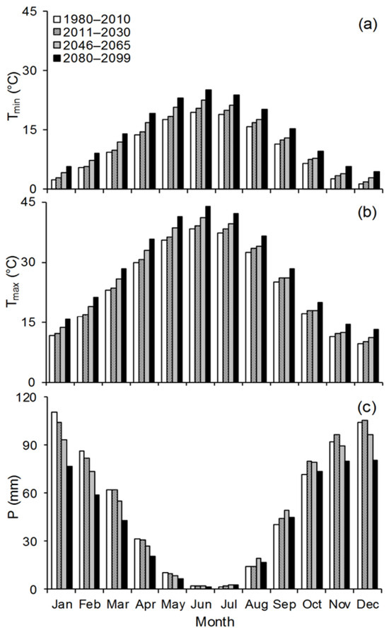
Figure 5.
Values of the monthly means of the minimum and maximum air temperature and precipitation (a) Tmin; (b) Tmax; (c) P, respectively, during the 1980–2010, 2010–2030, 2046–2065, and 2080–2099 period, downscaled by seven assembly general circulation models (GCMs).
To explain the potential alterations throughout the three considered intervals, the average values of the meteorological data were computed using seven GCMs. Figure 6 visualized the outcomes. Figure 6a–h show the box–whisker plots for the minimum and maximum mean air temperature and precipitation variation values, respectively, which were downscaled by LARS-WG7 depending on the seven GCMs for the 2011–2030, 2046–2065, and 2080–2099 time periods, respectively. Every box–whisker plot represents data computed by one GCM. During the 2080–2099 time period, among the many GCMs for precipitation estimations, no consistent tendencies demonstrating variation were observed. GFDL-ESM4, HadGEM3-GC3-L1, INM-CM5-0, UKESM1-0-LL, and MPI-ESM1-2-LR produced precipitation values that were lower than those from the baseline period. However, all GCMs predicted higher Tmin and Tmax than those from baseline 1 (1980–2010), illustrating little variation in estimates from the considered GCMs, demonstrating that there are minimal changes in predicting future severe temperatures by one single GCM. In contrast to the simulations for 2080–2099, the estimates for other intervals by the seven GCMs showed consistent alteration tendencies. Estimations of minimum and maximum air temperatures are greater compared to those in the 1980–2010 (baseline 1) interval, and the temperature calculations by the seven GCMs show increasing tendencies, especially during the 2080–2099 intervals compared to the baseline 1 (1980–2010) climate.
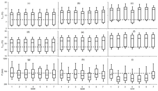
Figure 6.
The box plot shows the changes in (a–c) minimum temperature (Tmin), (d–f) maximum temperature (Tmax), and (g–i) precipitation (P) over the studied basin, downscaled from the seven GCMs using LARS-WG7 during the time horizons 2011–2030, 2046–2065, and 2080–2099 compared to 1980–2010. Note: (1) CNRM-CM6-1: Centre National de Recherché France, (2) GFDL-ESM4 = Geophysical Fluid Dynamics Lab USA, (3) HadGEM3-GC3-L1 = Meteorological Office UK, (4) INM-CM5-0 = Institute for Numerical Mathematics Russia, (5) UKESM1-0-LL = Meteorological Office UK, (6) MPI-ESM1-2-LR = Planck Institute for Meteorology Germany, (7) CESM2 = National Centre for Atmospheric USA.
3.2.2. Hydro-Climatic Drought Alteration Identification
Based on the annual reference period, RDIst and SDI indices are estimated to examine the interaction between meteorological and hydrological droughts, and are then correlated with each other (Figure 7). The linear regression equation shows relatively good fits between SDI and RDIst, as indicated by the relatively high correlation coefficient. This rather simple method yields outcomes with considerable ambiguity but is rather practical. This is because practical processes to moderate drought effects are categorically based on the severity category regarding the estimated drought occurrence, rather than the entire SDI assessment. To measure the amount of weather and hydrological drought events over the representative region during the future period, RDIst and SDI were computed using the measured and modeled hydro-climatic data. Figure 7a–h show the indices computed during baseline 1 (1980–2010) as well as the three considered future intervals, respectively, which are linked with the annual PET and Pav. Irregular recurring compositions of drought and wet periods have been identified during all periods. In general, drought phenomena, whether they are meteorological or hydrological, frequently arise when potential evapotranspiration increases, and precipitation decreases, and vice versa. Frequently, this event occurs during the commencement of the wet interval, which is indicated by either an increase in potential evapotranspiration linked with a precipitation reduction or a suspension in precipitation periods. As the RDIst and SDI examination reveals, it is expected that drought severity will significantly deteriorate in the future. In particular, in the interval 2080–2099, the severity of drought is expected to increase when months with total intervals of precipitation deficiencies and potential evapotranspiration expansions increase.
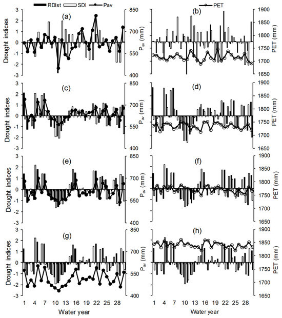
Figure 7.
Temporal variations of RDIst (the annual standardized reconnaissance drought index) and SDI (annual streamflow index) linked with Pav (the long-term mean basin precipitation) (left graphs) and PET (potential evapotranspiration) (right graphs) for: (a,b) 1980–2010; (c,d) 2011–2030; (e,f) 2046–2065; and (g,h) 2080–2099 time horizon, respectively, over the representative basin.
Regarding the streamflow alteration, the following has been obtained from the IHA simulation. During the baseline (1980–2010) and GCMs scenarios, various temporal yearly maximum values (i.e., 1-, 3-, 7-, 30-, and 90-days) are computed. The hydrological change extends from low to high in group no. 1. Table 5 shows that low amounts are detected in October, March, April, May, and September. November and December exhibit positive lowest levels of change. A minor change is likely in the intervals 2011–2030 and 2046–2065, whereas a modest change is noticed in 2080–2099, with nearly all months between March and September showing changes of approximately −36 to −42; see Table 5. The more severe lowest discharges display small variations in group no. 2. A small variation of approximately −28% is correlated with a 7-day lowest discharge for the 2080–2099 horizon. Concerning severe maximum discharges, group no. 2 exhibits low to modest variations. A modest variation of approximately −38% is related to 1- and 3-day peak discharges during the 2080–2099 horizon. Modest changes range between −36 and −38% and are related to 1-, 3-, and 30-day maximum flows for the 2080–2099 interval.

Table 5.
Hydrological alteration for the middle range of the variability approach (RVA) category for the Lower Zab River for the three future time periods compared to the baseline (1980–2010).
The temporal percentiles typically refer to the possible alterations in the hydrological properties of the basin and are, therefore, considered a fundamental numerical tool. This research estimates the 10th, 25th, 50th, 75th, and 90th percentiles, which measure the extent of peak discharge thresholds during the 1980–2010 baseline, and under the GCM scenario (Figure 8). The interval 2080–2099 is related to the biggest change. Figure 8a shows that the values of the monthly discharge are the same or larger than the threshold at 10% of the interval displaying drops varying between −22% (February) and −35% (September) for the period 2080–2099. Positive anomalies are noticed during November, December, and January (Figure 5a). There are negative shifts of 10 and 38% in January and September, in this order, for the 25th monthly percentiles. The anomalies during November and December are 18 and 51%, respectively (Figure 8b). Figure 8c shows that the irregularities associated with the monthly middle discharges expand between −19 (January) and −42% (September), respectively. Positive anomalies are recorded during November and December. However, the lowest anomaly is observed in December (−3%) compared to the 75th percentile (Figure 8d), whereas the maximum fall of −42% is noted in September. Figure 5e reveals that during November and September, the 90th monthly percentiles range from −4% to −41%, respectively. The study outcomes indicate that climate change is likely to have a significant overall impact on water resources.
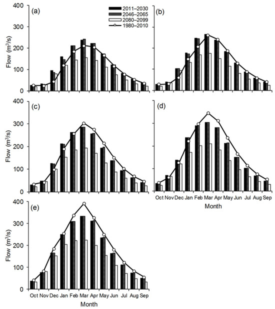
Figure 8.
Relationship linking the baseline with the climate change scenario for the monthly (a) 10th; (b) 25th; (c) 50th; (d) 75th; and (e) 90th percentiles.
3.2.3. Reservoir Inflow
The HBV model and climate change scenarios are calibrated over twelve years (1988–2000), with the validation period running from 1979 to 1986. Figure 9 depicts the values of the observations compared to the simulated streamflow time series by the HBV model for calibration (1988–2000) and validation (1979–1986), respectively. The statistical performance indicators—RMSE (root-mean-square error), IoA (index of agreement), r (correlation coefficient), MAE (mean absolute error), and NSCE (Nash–Sutcliffe) [3]—during the calibration stage of the considered HBV rainfall–runoff model, are 0.73, 0.99, 0.93, 0.65, and 80, respectively. The corresponding values during the validation period are 0.68, 0.99, 0.84, 0.60, and 50, respectively. The simulation results are promising, indicating that they can be confidently applied to future studies, such as running artificial climatic scenarios and estimating the relative change (%) in the average annual streamflow relative to normal climatic conditions.
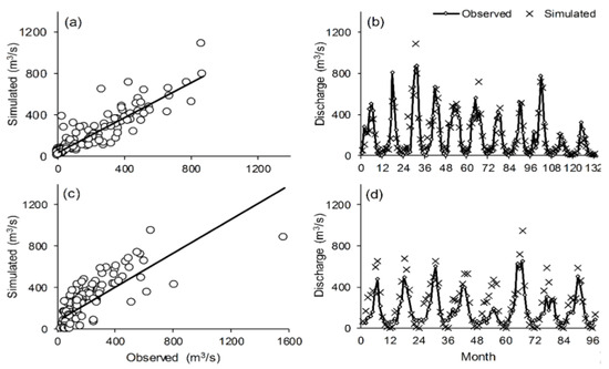
Figure 9.
Observations compared to the simulated streamflow time series using the Hydrologiska Byråns Vattenbalansavdelning model for (a,b) calibration periods (1988/1989–1999/2000) and (c,d) validation periods (1979/1980–1986/1987), respectively. Note: The solid line in (a,c) is a 45° line, representing what would be a perfect correspondence between observed data and solution values, the circle point.
Figure 10 presents temporal variations of the mean streamflow modeled by climate variables, estimated through GCM, and downscaled by LARS-WG7 (Figure 10a,c,e,g, left figures) and DP (Figure 10b,d,f,h, right figures) scenarios, respectively. To prevent any tendency caused by the rainfall–runoff model procedure, streamflow values for baseline 1 (1980–2010) and baseline 2 (1988–2000) correspond to the simulated values. The outcomes show how climate change is likely to lead to a reduction in reservoir inflow.
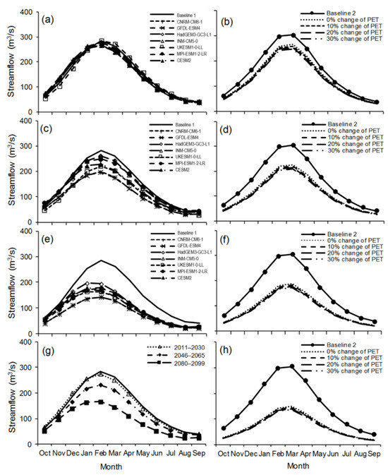
Figure 10.
The temporal and magnitude variations of the estimated average monthly Dokan reservoir inflow by the GCM (general circulation model) scenarios (left figures): (a) 2011–2030; (c) 2046–2065; and (e) 2080–2099 time periods; and (g) relationship between the three potential time periods, as compared to the values of baseline 1 (1980-2010); and delta perturbation scenarios (right figures): (b) 10%; (d) 20%; (f) 30%; and (h) 40% reduction in precipitation (P), respectively, as compared with the values of baseline 2 (1988–2000). Note: CNRM-CM6-1 = Centre National de Recherché France, GFDL-ESM4 = Geophysical Fluid Dynamics Lab USA, HadGEM3-GC3-L1 = Meteorological Office UK, INM-CM5-0 = Institute for Numerical Mathematics Russia, UKESM1-0-LL = Meteorological Office UK, MPI-ESM1-2-LR = Planck Institute for Meteorology Germany, CESM2 = National Centre for Atmospheric USA.
Generally, similar reductions are revealed in the estimated values of the mean monthly flow by GCM and DP scenarios, and, consequently, the simulated values of the maximum flow rates by both scenarios are almost identical. The entire GCM ensemble illustrates reductions in maximum values varying from 2% (UKESM1-0-LL) to 10% (GFDL-ESM4), as shown in Figure 10a, 12 to 37% (CNRM-CM6-1 and GFDL-ESM4) as indicated in Figure 10c, and 44 to 55% (HadGEM3-GC3-L1 and GFDL-ESM4) as illustrated in Figure 10e, during the considered potential intervals, respectively. In the 2020s, based on the downscaled meteorological parameters, there is an expected decline of approximately 6% in the average values, at a monthly timescale, of the surface runoff (Figure 10g), which is similar to the estimated values from the DP storyline (Future1 (F1): a 10% decrease in precipitation and 0% potential evapotranspiration), as shown in Figure 6a. The equivalent decline for the period 2046–2065 is projected at nearly 21%, which is equal to the estimated decline in streamflow through the DP scenario (F6: a 10% decrease and increase in precipitation and potential evapotranspiration, respectively), as seen in Figure 10a. Yet, the expected decline in the surface runoff for the third period is about 48% (Figure 10d), which is equal to the value obtained via Figure 10f (F16: a 30% precipitation reduction and 30% increase in potential evapotranspiration). Concerning the worst-case scenarios of DP and GCM, respectively, extensive changes in the inflow values of −10, −36, and −55% during August June, and July, respectively, are expected during the three considered intervals (Figure 10g), and in −56 to −58% are expected during the wet and dry intervals, respectively (Figure 10h). Furthermore, for the 2046–2065 future periods, peak flow rates were recorded previously than for the reference time interval since the delay time was approximately eight days. However, there was no alteration in the time to maximize the discharge that was estimated by other intervals or by DP.
3.2.4. Reservoir Performance
The demand for water in the future is supposed to be maintained without major changes to the baseline duration. The daily streamflow value simulation by the HBV model was used to imitate water resource development in the RCY model, simulating Dokan reservoir operations. Weather data for GCM and DP were downloaded using LARS-WG7. Subsequently, the indicator assessment (among other assessments) was applied to the climate change and baseline interval scenarios by running the RCY model.
Table 5 shows the reservoir volume needed to achieve the required water needs. The reservoir reliability was calculated for each model simulation and the climate change storyline. The consecutive OPOF% (reliability) series consists of a series of climate change impacts regarding the organization of water resources.
The findings enable the preparation of operational adaptation approaches. According to the inflow prediction and the existing status of the reservoir capacity, strategy makers can change the reservoir’s operational regulations. This can lead to more effective reservoir management. Table 6 shows the relationship between capacity (106 m3), yield (%), and reliability (OPOF), which were developed by applying the RCY model.

Table 6.
Statistical relationships between water yield (Y, %), the operational probability of (reservoir) failure (OPOF, %), reservoir capacity (C, 106 m3), and Y% using seven global circulation models (GCMs) and three future time periods.
4. Discussion
The downscaling LARS-WG7 model is an accurate representation of meteorological variables on a daily timescale; it is used to estimate potential internals. The findings show that temperatures at all ten weather stations are expected to rise by a mean of 0.55–4.53 °C during the studied time. However, the wide variation is due to the study’s use of various emission scenarios, and the uncertainty of the downscaling process may have also impacted the projected results. These findings are consistent with previous research conducted in the climatic region [33,34]. The increase is moderate in Iraq’s northern parts of the country, but more so in the central, western, and southern regions. Temperature increases in Iraq have the potential to accelerate desertification, affecting agriculture [35], land use/land cover changes, and water supplies [22]. Rising surface water evaporation is leading to water scarcity, highlighting the urgent need for sustainable, long-term solutions to address and adapt to these consequences. Climate fluctuations significantly contribute to the increase in sand and dust storms, as well as other extreme weather events, which have recently impacted regions in Iraq [35].
Moreover, precipitation is expected to decrease by about 6.32, 17.33, and 340.18 mm during the three potential intervals, with relative changes varying monthly. These findings about decreasing annual precipitation are consistent with earlier research [34]. The anticipated variations in the amount, intensity, and frequency, of future rainfall measures pose threats to organizational resilience, potentially resulting in drought episodes.
Climate change is a complex challenge that goes beyond simple shifts in weather patterns. Economic, environmental, and social factors all influence societal progress. Effectively addressing the implications of climate change requires proactive efforts from various socioeconomic groups within the affected region. Adaptation and mitigation strategies include water management, comprehensive national water resource management and planning, restoration of water treatment infrastructure, and the use of alternative water sources, such as recycled wastewater via water recycling plants and water harvesting. To improve environmental quality and reduce greenhouse gas emissions, it is essential to invest in renewable energy opportunities and implement green infrastructure solutions, like solar and wind power.
5. Conclusions and Recommendations
Recent research has shown that climate change is one of the most urgent environmental concerns, specifically the rising temperatures in arid and semi-arid areas. The current study presents a comprehensive and broad research methodology that could help improve climate change adaptation policies:
- The downscaling model, LARS-WG7, provides better estimations of meteorological variables on a daily timescale, so it could be used to estimate potential internal values.
- Tmin and Tmax are projected to increase by nearly 0.54, 3.03, and 4.36 °C, and 0.56, 2.49, and 4.70 °C, respectively, between 2011–2010, 2046–2065, and 2080–2099. Conversely, precipitation is expected to decrease by about 6.32, 17.33, and 340.18 mm during the three potential intervals, with the relative changes varying monthly.
- During the 2080–2099 period, no consistent trend has been noted among several GCM precipitation calculations. GFDL-ESM4, HadGEM3-GC3-L1, INM-CM5-0, UKESM1-0-LL, and MPI-ESM1-2-LR forecasted lower precipitation values compared to those in the baseline 1 interval predictions.
- There have been minimal changes in predicting the potential maximum temperature using a single GCM. The estimates from seven GCMs of these extremes during the 2046–2065 and 2046–2065 intervals show consistent change tendencies, in contrast to the extremes projected for the 2080–2099 interval.
- In general, the estimated monthly flow values for the GCM and DP scenarios show similar reductions; thus, the estimated maximum flow rates for both scenarios are nearly identical. The expected runoff reduction from 2080 and 2099 is around 48%, comparable to the discharges caused by DP (F16: a 30% increase in potential evapotranspiration and a 30% decrease in precipitation, for example).
- Precipitation reduction leads to increased drought episode periods (after 1999).
- Irregular periodic features of wet and dry intervals are predicted in the baseline and potential intervals.
- The severity of hydro-climatic droughts will noticeably deteriorate in the future, especially in the 2080–2099 interval. The severity of the drought will increase when the periods of extended potential evapotranspiration increase, and precipitation deficiencies rise.
- During the 2080–2099 time spans, modest differences varying between −36 and −38% are observed for the 1-, 3-, and 30-day highest discharges.
- The impact of climate change will extend the flood-free period.
- In general, the climate change effect on the estimation of discharge values reflects its influence on the annual maximum values. As a result, the estimated values of low and high annual streamflow will decrease due to reduced precipitation and surface runoff.
- The monthly discharge was the same as or exceeded the critical values at 10% of the interval, displaying reductions varying between −22% (February) and −35% (September) during the 2080–2099 interval.
The findings present a solid base for climate change adaptation, considering as many climatic storylines as possible. Additionally, artificial storylines would be enhanced via GCM scenarios, as they allow for an extensive range of probable regional climate change scenarios and are simpler to make and use. Furthermore, the current research has to be replicated for more regions and climates, which would provide an additional overview of the study conclusions.
6. Limitations of the Study
Although the current study has achieved its main research objective, there are many restrictions. Firstly, the simple standard technique was achieved, based on just three rainfall–runoff simulations and 35 hydrological years of daily flow rate data. Adding more rainfall–runoff simulations and further observations could improve the results of the multi-model grouping presentation. Then, as a result of the unavailability of several meteorological data, such as solar circulation, relative moisture, and wind speed, the Hargreaves technique has been applied to calculate the basin’s potential evapotranspiration, with the intention that when the long-term consistent weather data of many climate variables are available, the PM method will be considered. Thirdly, to examine the RDI index sensitivity to the potential evapotranspiration estimation method, the current research depends on a dataset of just 24 weather stations, indicating a variety of altitudes and weather environments. So, to address the proposed conclusions, the use of further weather stations is recommended.
Author Contributions
Conceptualization, R.M.; methodology, R.M.; software, R.M.; validation, R.M.; formal analysis, R.M.; investigation, R.M.; resources, R.M.; data curation, R.M.; writing—original draft preparation, R.M.; writing—review and editing, M.S.; visualization, R.M.; supervision, M.S.; project administration, M.S.; funding acquisition, M.S. All authors have read and agreed to the published version of the manuscript.
Funding
This research received no external funding.
Institutional Review Board Statement
Not applicable.
Informed Consent Statement
Not applicable.
Data Availability Statement
Dataset available upon request from the authors. The data are not publicly available due to privacy.
Acknowledgments
The main author obtained financial support from the Iraqi Government via a Ph.D. studentship.
Conflicts of Interest
Miklas Scholz was employed by the companies Kunststoff-Technik Adams and Nexus by Sweden. The remaining author declares that the research was conducted in the absence of any commercial or financial relationships that could be construed as a potential conflict of interest.
References
- IPCC (Intergovernmental Panel on Climate Change). Climate Change 2014: Impacts, Adaptation, and Vulnerability. Available online: http://www.ipcc.ch/report/ar5/wg2 (accessed on 15 May 2017).
- Mohammed, R.; Scholz, M. The reconnaissance drought index: A method for detecting regional arid climatic variability and potential drought risk. J. Arid Environ. 2017, 144, 181–191. [Google Scholar] [CrossRef]
- Mohammed, R.; Scholz, M.; Nanekely, M.A.; Mokhtari, Y. Assessment of models predicting anthropogenic interventions and climate variability on surface runoff of the Lower Zab River. Stoch. Environ. Res. Risk Assess. 2018, 32, 223–240. [Google Scholar] [CrossRef]
- Mohammed, R.; Scholz, M. Climate variability impact on the spatiotemporal characteristics of drought and Aridity in arid and semi-arid regions. Water Resour. Manag. 2019, 33, 5015–5033. [Google Scholar] [CrossRef]
- Park, J.Y.; Kim, S.J. Potential impacts of climate change on the reliability of water and hydropower supply from a multipurpose dam in South Korea. J. Am. Water Resour. Assoc. (JAWRA) 2014, 50, 1273–1288. [Google Scholar] [CrossRef]
- Reis, J.; Culver, T.B.; Block, P.J.; McCartney, M.P. Evaluating the impact and uncertainty of reservoir operation for malaria control as the climate changes in Ethiopia. Clim. Change 2016, 136, 601–614. [Google Scholar] [CrossRef]
- Trzaska, S.; Schnarr, E. A Review of Downscaling Methods for Climate Change Projections; United States Agency for International Development by Tetra Tech ARD, Burlington, Vermont, 2014; Volume 45, pp. 45–2621.
- Semenov, M.A.; Pilkington-Bennett, S.; Calanca, P. Validation of ELPIS 1980-2010 baseline scenarios using the observed European Climate Assessment data set. Clim. Res. 2013, 57, 1–9. [Google Scholar] [CrossRef]
- McMahon, T.A.; Adeloye, A.J.; Zhou, S.L. Understanding performance measures of reservoirs. J. Hydrol. 2006, 324, 359–382. [Google Scholar] [CrossRef]
- Vicuna, S.; Dracup, J.A. The evolution of climate change impact studies on hydrology and water resources in California. Clim. Change 2007, 82, 327–350. [Google Scholar] [CrossRef]
- Minville, M.; Brissette, F.; Krau, S.; Leconte, R. Adaptation to climate change in the management of a Canadian water-resources system exploited for hydropower. Water Resour. Manag. 2009, 23, 2965–2986. [Google Scholar] [CrossRef]
- Lim, K.J.; Park, Y.S.; Kim, J.; Shin, Y.C.; Kim, N.W.; Kim, S.J.; Jeon, J.H.; Engel, B.A. Development of generic algorithm-based optimisation module in WHAT system for hydrograph analysis and model application. Comput. Geosci. 2010, 36, 936–944. [Google Scholar] [CrossRef]
- Vano, J.A.; Scott, M.J.; Voisin, N.; Stöckle, C.O.; Hamlet, A.F.; Mickelson, K.E.; Elsner, M.M.; Lettenmaier, D.P. Climate change impacts on water management and irrigated agriculture in the Yakima River Basin, Washington, USA. Clim. Change 2010, 102, 287–317. [Google Scholar] [CrossRef]
- Ludwig, F.; Slobbe, E.V.; Cofino, W. Climate change adaptation and integrated water resource management in the water sector. J. Hydrol. 2014, 518, 235–242. [Google Scholar] [CrossRef]
- Chen, J.; Brissette, F.P.; Leconte, R. The uncertainty of downscaling method in quantifying the impact of climate change on hydrology. J. Hydrol. 2011, 401, 190–202. [Google Scholar] [CrossRef]
- Tigkas, D.; Vangelis, H.; Tsakiris, G. Drought and climatic change impact on streamflow in small watersheds. Sci. Total Environ. 2012, 440, 33–34. [Google Scholar] [CrossRef]
- Mohammed, R.; Scholz, M. Adaptation strategy to mitigate the impact of climate change on water resources in arid and semi-arid regions: A case study. Water Resour. Manage. 2017, 31, 3557–3573. [Google Scholar] [CrossRef]
- Semenov, M.A.; Barrow, E.M.; Lars-Wg, A. A Stochastic Weather Generator for Use in Climate Impact Studies; User Man Herts UK; 2002; pp. 1–27.
- Information Technology Services (ITS). IBM SPSS statistics 23 Part 3: Regression Analysis. Winter 2016, Version 1. 2016. Available online: https://www.ibm.com/support/pages/downloading-ibm-spss-statistics-23 (accessed on 29 May 2023).
- Allen, R.G.; Pereira, L.S.; Raes, D.; Smith, M. Crop evapotranspiration: Guidelines for computing crop water requirements. In Food and Agriculture Organization (FAO) Irrigation and Drainage Paper 56, 1st ed.; FAO: Rome, Italy, 1998. [Google Scholar]
- FAO. Food and Agriculture Organization of the UN. Adaptation to Climate Change in Semi-Arid Environments. Experience and Lessons from Mozambique; Environment and Natural Resources Management Series; FAO: Rome, Italy, 2012; pp. 1–83. Available online: http://www.fao.org/docrep/015/i2581e/i2581e00.pdf (accessed on 18 June 2017).
- Mahdi, Z.A.; Mohammed, R. Land use/land cover changing aspect implications: Lesser Zab River Basin, northeastern Iraq. Environ. Monit. Assess. 2022, 194, 652. [Google Scholar] [CrossRef]
- Mohammed, R.; Scholz, M. Impact of climate variability and streamflow alteration on groundwater contribution to the base flow of the Lower Zab River (Iran and Iraq). Environ. Earth Sci. 2016, 75, 1392. [Google Scholar] [CrossRef]
- Mohammed, R.; Scholz, M. Impact of evapotranspiration formulations at various elevations on the reconnaissance drought index. Water Resour. Manage. 2017, 31, 531–538. [Google Scholar] [CrossRef]
- Tsakiris, G.; Vangelis, H. Establishing a drought index incorporation evapotranspiration. Eur. Water 2005, 9, 3–11. [Google Scholar]
- Vangelis, H.; Tigkas, D.; Tsakiris, G. The effect of PET method on Reconnaissance Drought Index (RDI) calculation. J. Arid. Environ. 2013, 88, 130–140. [Google Scholar] [CrossRef]
- McMahon, T.A.; Adeloye, A.J. Water Resources Yield; Water Resources Publications: Littleton, CO, USA, 2005. [Google Scholar]
- Moy, W.; Cohon, J.L.; ReVelle, C.S. A programming model for analysis of the reliability, resilience, and vulnerability of a water supply reservoir. Water Resour. Res. 1986, 22, 489–498. [Google Scholar] [CrossRef]
- Fowler, H.J.; Kilsby, C.G.; Connell, P.E.O. Modeling the impacts of climatic change and variability on the reliability, resilience, and vulnerability of a water resource system. Water Resour. Res. 2003, 39, 1222. [Google Scholar] [CrossRef]
- Soundharajan, B.S.; Adeloye, A.J.; Remesan, R. Evaluating the variability in surface water reservoir planning characteristics during climate change impacts assessment. J. Hydrol. 2016, 538, 625–639. [Google Scholar] [CrossRef]
- Semenov, M.A.; Stratonovitch, P. Use of multi-model ensembles from global climate models for assessment of climate change impacts. Clim. Res. 2010, 41, 1–14. [Google Scholar] [CrossRef]
- Mahjour, S.K.; Liguori, G.; Faroughi, S.A. Selection of representative general circulation models under climatic uncertainty for Western North America. J. Water Clim. Change 2024, 15, 686–702. [Google Scholar] [CrossRef]
- Mohammed, R.; Scholz, M. Climate change and water resources in arid regions: Uncertainty of the baseline time period. Theor. Appl. Climatol. 2019, 137, 1365–1376. [Google Scholar] [CrossRef]
- Mohammed, D.R.; Mohammed, R.K. Climate Change’s Impacts on Drought in Upper Zab Basin, Iraq: A Case Study. Tikrit J. Eng. Sci. 2024, 31, 161–171. [Google Scholar] [CrossRef]
- Hassan, W.H.; Nile, B.K.; Kadhim, Z.K.; Mahdi, K.; Riksen, M.; Thiab, R.F. Trends, forecasting and adaptation strategies of climate change in the middle and west regions of Iraq. SN Appl. Sci. 2023, 5, 312. [Google Scholar] [CrossRef]
Disclaimer/Publisher’s Note: The statements, opinions and data contained in all publications are solely those of the individual author(s) and contributor(s) and not of MDPI and/or the editor(s). MDPI and/or the editor(s) disclaim responsibility for any injury to people or property resulting from any ideas, methods, instructions or products referred to in the content. |
© 2024 by the authors. Licensee MDPI, Basel, Switzerland. This article is an open access article distributed under the terms and conditions of the Creative Commons Attribution (CC BY) license (https://creativecommons.org/licenses/by/4.0/).