Article

Construction and Validation of Surface Soil Moisture Inversion Model Based on Remote Sensing and Neural Network

1
State Key Laboratory of Watershed Water Cycle Simulation and Regulation, China Institute of Water Resources and Hydropower Research, Beijing 100038, China
2
Zhejiang Institute of Hydraulics & Estuary (Zhejiang Institute of Marine Planning and Design), Hangzhou 310020, China
3
College of Land Science and Technology, China Agricultural University, Beijing 100083, China
*
Author to whom correspondence should be addressed.
Atmosphere 2024, 15(6), 647; https://doi.org/10.3390/atmos15060647
Submission received: 10 April 2024 / Revised: 8 May 2024 / Accepted: 16 May 2024 / Published: 28 May 2024
(This article belongs to the Section Biosphere/Hydrosphere/Land–Atmosphere Interactions)

Abstract

:
Surface soil moisture (SSM) reflects the dry and wet states of soil. Microwave remote sensing technology can accurately obtain regional SSM in real time and effectively improve the level of agricultural drought monitoring, and it is of great significance for agricultural precision irrigation and smart agriculture construction. Based on Sentinel-1, Sentinel-2, and Landsat-8 images, the effect of vegetation was removed by the water cloud model (WCM), and SSM was retrieved and validated by a radial basis function (RBF) neural network model in bare soil and vegetated areas, respectively. The normalized difference vegetation index (NDVI) calculated by Landsat-8 (NDVI_Landsat-8) had a better effect on removing the influence the of vegetation layer than that of NDVI_Sentinel-2. The RBF network model, established in a bare area (R = 0.796; RMSE = 0.029 cm3/cm3), and the RBF neural network model, established in vegetated areas (R = 0.855; RMSE = 0.024 cm3/cm3), have better simulation effects on SSM than a linear SSM inversion model with single polarization. The introduction of surface parameters to the RBF neural network model can improve the accuracy of the model and realize the high-accuracy inversion of SSM in the study area.

1. Introduction

Soil moisture is an important part of the Earth’s water resources and land productivity and is also a key factor in the study of the hydrological cycle and climate change [1]. Soil moisture monitoring at a regional scale is of great significance for the study of the surface water cycle [2], agricultural drought [3], flood assessment [4], and crop yield estimation [5]. Monitoring soil moisture helps to understand the energy and carbon cycles and to simulate many meteorological, climatic, and hydrological factors [6,7,8]. At the same time, the study of soil moisture is of great significance for improving regional climate and agricultural irrigation management [9].
Surface soil moisture (SSM) is an important part of soil water content. Traditional SSM measurement methods are based on drying methods and sensors, which are suitable for point-scale SSM collection [10]. The development of remote sensing technology has made the large-scale and rapid measurement of SSM a reality. Compared with the traditional methods of measuring SSM, remote sensing monitoring is efficient and cost-effective, and the accuracy can also meet application requirements. At present, the use of remote sensing to invert SSM is mainly divided into two methods: optical remote sensing and microwave remote sensing. Commonly used optical remote sensing methods include the thermal inertia method, the crop water deficit index method, and the temperature vegetation drought index method [11,12], but optical remote sensing is susceptible to rain, clouds, and other weather effects, and the data quality is not controllable. Compared with optical remote sensing, the band of microwave remote sensing is wider and less affected by clouds and rain, can realize all-weather monitoring, and can penetrate the vegetation layer with microwave signals to reach the soil surface. More and more scholars pay attention to the use of microwave remote sensing to invert SSM [13]. There are differences in the modeling of SSM in bare soil and vegetated areas, and the effect of vegetation needs to be removed for the inversion of SSM in vegetated areas. Currently, the inversion models of SSM in bare soil include the Oh model [14], the IEM model [15], the Dubois model [16], the AIEM model [17], etc. The inversion model of SSM in vegetated areas is different from that of bare soil, and the inversion of SSM in vegetated areas needs to remove the influence of vegetation. SSM inversion models for vegetated areas include the MIMICS model [18], which has to be considered for its generalizability, higher number of input parameters, and high requirements for in situ surface parameters. The water cloud model (WCM) [19], on the other hand, is relatively simple and has fewer input parameters, and most of the parameters can be replaced using remote sensing estimates. In recent years, more computer algorithms have been introduced into the SSM inversion model, such as neural networks [20], support vector machines [21], etc., all of which perform well. Among them, the RBF neural network model has a strong approximation ability, a fast learning convergence speed, and a simple structure, and it can solve the nonlinear function problem [22].
In vegetated areas, Lu et al. [23] used change-monitoring technology to study the phase and amplitude of synthetic aperture radar (SAR) images in the south of France, aiming to explore the sensitivity of the two to changes in SSM covered by sparse vegetation. The results showed that change-monitoring technology can successfully capture changes in SSM, which range from 0.05 to 0.20 cm3/cm3. At the same time, the amplitude and phase information should be considered comprehensively when using SAR images to invert SSM so as to improve the inversion accuracy. Lievens et al. [24] used a combination of the WCM and IEM models to build a scattering model under winter wheat cover. By fixing the root mean square height, they reduced variations in soil roughness parameters and improved the accuracy of SSM inversion. Experimental results from wheat fields in Belgium showed that the introduction of effective roughness parameters could significantly improve the accuracy of SSM inversion on the underlying wheat surface, and it was suggested that leaf area index (LAI) should be used as a vegetation index. In order to eliminate the influence of vegetation on SSM retrieval, Bao et al. [25] established a VWC estimation model using the Landsat-8 spectral index and combined it with WCM to construct a modified WCM for retrieving the SSM covered by vegetation. The model has been applied in the United Kingdom and Spain. Compared with Sentinel-1 VH polarization, VV polarization is more advantageous in SSM inversion, with an R of 0.911 and an RMSE of 0.053 cm3/cm3 between the model inversion values and the in situ values. In bare soil, Chen et al. [26] proposed an improved algorithm based on the fusion data of multi-frequency amplitude and phase migration based on principal component analysis (PCA) and the entropy method for SSM inversion. Compared with the inversion of SSM by GPS and the Beidou satellite, the inversion of SSM obtained by this method had a stronger correlation with the in situ SSM. RMSE was reduced by 50.93%, and the average R increased by 11.71%.
Taking Daxing District, China, as an example, based on Sentinel-1, Sentinel-2, and Landsat-8 images, in this study, the WCM removes the influence of vegetation, and then, the RBF neural network model is used to establish an inversion model of SSM in bare soil and vegetated areas and then compare and analyze the model with a linear SSM inversion model based on the polarization of VV and VH and validate the inversion model. By integrating multi-source data, the WCM and RBF neural network can be used to realize the high-precision inversion of SSM in the study area, which is an important reference value for guiding the construction of precision irrigation and agricultural modernization. The use of remote sensing technology can accurately and real-time monitor SSM at a regional scale and improve the efficiency of limited water resources for irrigation. It is of great significance to the development of China’s agricultural economy, the implementation of water-saving irrigation, and the construction of smart agriculture.

2. Data and Methodology

2.1. Study Area

Daxing District is located in the southern part of Beijing, in the northern part of the North China Plain between 39°26′ N–39°50′ N and 116°13′ E–116°43′ E (Figure 1), with an altitude of 5–75 m. The climate is a warm-temperate semi-moist continental monsoon climate with four distinct seasons. The average monthly temperature in summer is 25.9 °C; the average monthly temperature in winter is −5 °C. The average annual frost-free period is 181 d; the average annual precipitation is 569.4 mm. The rainfall is concentrated in June–August [27]; the average annual sunshine hours are 2764 h. The soil types in Daxing District include wind–sand soil, brown soil, tidal soil, rice soil, and swampy soil. The main food crops grown are wheat and corn.

2.2. Data

2.2.1. Sentinel-1

The European Space Agency (ESA) launched Sentinel-1A and Sentinel-1B in the Copernicus program. The Sentinel-1 satellite is a C-band (5.405 GHz, 5.6 cm) radar imaging system for the European polar orbit, with a single-satellite temporal resolution of 12 d. The Sentinel-1 data used in this study are L1-level single look complex (SLC) products acquired in interferometric wideband (IW) mode, with a spatial resolution of 5 m × 20 m, and polarization modes VV and VH. The data were obtained from https://scihub.copernicus.eu/ (accessed on 1 May 2023), and the acquisition dates are shown in Table 1. The pre-processing of Sentinel-1 images included multilooking, atmospheric correction, filtering, and geometric correction. This is achieved using the Sentinel-1 toolbox (S1TBX) tool in the SNAP software provided by the ESA. To remove speckle noise, Refined Lee [28] was selected to filter the image. Finally, the images were resampled to 20 m.

2.2.2. Sentinel-2

The Sentinel-2 consists of Sentinel-2A and Sentinel-2B, with a temporal resolution of 10 d. The satellite carries a multispectral instrument (MSI) with 13 bands; a spectral range of 0.4–2.4 μm; spatial resolutions of 10, 20, and 60 m; and a width of 290 km. It can provide information on the growth of land vegetation, soil cover, and the environment of inland rivers and coastal areas. In this study, Sentinel-2A images were used to calculate the normalized differential vegetation index (NDVI) and normalized differential water index (NDWI). The images were obtained from https://scihub.copernicus.eu/ (accessed on 7 May 2024), and the acquisition date is shown in Table 1. The images are the L1C atmospheric apparent reflectance product after orthophoto correction and subpixel-level geometric precision correction. The Sentinel-2A images were radiometrically calibrated and atmospherically corrected using the Sen2cor tool provided by the ESA and uniformly resampled to a spatial resolution of 20 m.

2.2.3. Landsat-8

The Landsat-8 satellite was launched in 2013 by the National Aeronautics and Space Administration (NASA) and carries an operational land imager (OLI) and a thermal infrared sensor (TIRS), with a temporal resolution of 16 d. The OLI includes nine bands with a spatial resolution of 30 m and one panchromatic band with a resolution of 15 m, and the imaging width is 185 km × 185 km. The TIRS consists of two separate thermal infrared bands with a resolution of 100 m. In this study, OLI images were used, with a spectral range of 0.43 to 12.51 μm. The images were obtained from https://glovis.usgs.gov/ (accessed on 7 May 2024), and the acquisition date is shown in Table 1. The ENVI 5.3 software was used to perform radiometric calibration, atmospheric correction, and clipping. Finally, the images were resampled to 20 m.
Due to the concentration of bare soil and vegetated areas in the study area, buildings and non-agricultural areas have been removed. Therefore, after the Sentinel-1, Sentinel-2, and Landsat-8 images were uniformly resampled to a spatial resolution of 20 m, the resolution clearly expressed the characteristics of the underlying surface in the study area.

2.2.4. Surface Soil Moisture

In order to establish the RBF neural network model and linear model and validate the accuracy of the models, the “Handheld ProCheck + GS3” instrument was used to measure SSM. A cultivated field with open terrain and no obstacles around was selected as the sampling point. SSM was measured at four points evenly around the measuring point at the center of the circle and with a radius of 1 m; the average SSM at five points was taken as the actual SSM at the point; and the coordinates of the latitude and longitude of the point were recorded with the use of the global positioning system (GPS). Each sampling point was spaced at least 20 m. The data acquisition dates are shown in Table 1.

2.3. Methodology

2.3.1. Water Cloud Model

The water cloud model (WCM) is a proposed SSM inversion model for low-vegetation areas based on radiative transfer theory [19]. The WCM assumes the vegetation layer is composed of water droplets of uniform size and thickness, randomly covering the ground surface; only a single scattering between the vegetation and the ground surface is considered, and diffuse scattering between the ground surface and the vegetation is ignored [29]. The model divides the total backscattering into two parts: soil backscattering and vegetation backscattering. There is also multiple scattering between the vegetation and soil. Multiple scattering between the vegetation and soil is often ignored [30,31]. The WCM is expressed as
σ = σ veg + T 2 σ soil
σ veg = A V W C cos θ 1 T 2
T 2 = exp 2 B V W C sec θ
where σ is the total backscattering (dB); σveg is the vegetation backscattering (dB); σsoil is the soil backscattering (dB); θ is the radar angle of incidence (°); VWC is the vegetation water content (kg/m2); A and B depend on the type of vegetation and the frequency of the incident electromagnetic wave. Bindlish and Barros [32] have summarized the parameters of A and B in water cloud modeling in use scenarios. According to the actual surface cover of Daxing District, the comprehensive use mode is selected; i.e., A = 0.0012, and B = 0.091. The VWC can be characterized by the NDVI and NDWI. Jackson et al. [33,34] established the relationship between the VWC and the NDVI and NDWI as follows:
V W C = 1.913 NDVI 2 0.3215 NDVI
V W C = 1.44 NDWI 2 + 1.36 NDWI + 0.34
The NDVI and NDWI were calculated using Sentinel-2 and Landsat-8 images, respectively. The formulae are as follows:
NDVI = R NIR R RED R NIR + R RED
NDWI = R NIR R SWIR R NIR + R SWIR
where RNIR is the reflectance in the near-infrared band; RRED is the reflectance in the red band; RSWIR is the reflectance in the short-wave infrared band.

2.3.2. RBF Neural Network Model

The neural network is a model formed in a simplified way that mimics the way neurons in the brain process information and consists of a large number of neurons interconnected with each other. Each neuron represents a specific output function called an excitation function. A signal input between two neighboring neurons produces a weighted value called a weight. The radial basis function (RBF) neural network model has the advantage of strong global approximation ability and can overcome the local minima problem. In addition, the RBF neural network model has the advantages of fast learning convergence and a simple structure, and it can solve nonlinear function problems. The RBF neural network is invoked in MATLAB 2020.
net = newrb P ,   T ,   GOAL ,   SPREAD ,   MN ,   DF
where P is the input vector; T is the output vector; GOAL is the root mean square error objective, and it is set to 0.01 [35]; MN is the maximum number of neurons, that is, the number of input vectors; DF is the display frequency of the training process, and the default value is 25. The experiment shows that, when the SPREAD is 0.2, the RBF network has the smallest error and the best approximation effect.
In vegetated areas, there are 220 input vectors, and the model randomly selects 200 to train the RBF neural network model and 20 to judge the correlation between the output results and the in situ SSM. In bare soil, there are 136 input vectors, 120 of which are randomly selected by the model to train the RBF neural network model, and 16 data are used to judge the correlation between the output results and the in situ SSM.

2.3.3. Statistical Metrics

In order to evaluate the SSM inversion results of the RBF neural network model and the linear model, correlation coefficient (R) and root mean square error (RMSE) were used for accuracy validation.
R = i = 1 n P i P ¯ O i O ¯ i = 1 n P i P ¯ 2 i = 1 n O i O ¯ 2
RMSE = i = 1 n O i P i 2 n
where n is the number of the validation value; Oi and Pi are the in situ SSM and estimated SSM, respectively; P ¯ is the average of the estimated values; O ¯ is the average of the in situ values.

3. Results

3.1. Evaluation of the Effectiveness of Water Cloud Modeling in Removing the Impact of Vegetation Layers

Figure 2 shows the comparative results of the NDVI removal effects calculated by different remote sensing images in VV polarization. For the convenience of description, the NDVI and NDWI calculated by the Sentinel-2 and Landsat-8 images are abbreviated as NDVI_Sentinel-2, NDWI_Sentinel-2, NDVI_Landsat-8, and NDWI_Landsat-8. The VWC calculated by NDVI_Sentinel-2 is substituted into the WCM, and the results show that the reduction in backscattering in VV polarization is in a range of 0.05–1.7 dB. The average value of the contribution of the vegetation layer to the total backscattering in VV polarization is 0.9 dB, and the average total backscattering in VV polarization is −9.59 dB. The results of the VWC substitution into the WCM computed by NDVI_Landsat-8 show that the reduction range of the backscattering in VV polarization is 0.03–2.59 dB; the average value of the contribution of the vegetation layer to the total backscattering in VV polarization is 1.29 dB; and the average total backscattering in VV polarization is −9.59 dB. The average total backscattering is −9.97 dB.
Figure 3 shows the comparison results of NDWI’s effect on vegetation removal calculated with different remote sensing images in VV polarization. NDWI_Sentinel-2 calculates the VWC substitution into the WCM; the results show that the range of the VV polarization attenuation values is 0.018–0.093 dB, the average value of the contribution of the vegetation layer to the total backscattering in VV polarization is 0.053 dB, and the average total backscattering in VV polarization is −8.73 dB. The NDWI_Landsat-8 calculation of VWC substituted into the WCM shows that the VV polarization attenuation values range from 0.022 to 0.26 dB, the average value of the contribution of the vegetation layer to the total backscattering in VV polarization is 0.115 dB, and the average total backscattering in VV polarization is −8.79 dB.
Figure 4 shows the comparative results of the NDVI removal effects calculated by different remote sensing images in VH polarization. For the NDVI_Sentinel-2 calculation of VWC substitution into the WCM, the results show that the range of VH polarization attenuation values is 0.2–3.01 dB; the average of the contribution of the vegetation layer to the total backscattering in VH polarization is 1.59 dB; and the average total backscattering in VH polarization is −16.75 dB. The VWC calculated by NDVI_Landsat-8 is substituted into the WCM; the results show that the VH polarization attenuation values range from 0.1 to 4.6 dB, the average value of the contribution of the vegetation layer to the total backscattering in VH polarization is 2.26 dB, and the average total backscattering in VH polarization is −17.42 dB.
Figure 5 shows the comparison results of NDWI’s effect on vegetation removal calculated by different remote sensing images in VH polarization. The results of the NDWI_Sentinel-2 calculation of VWC substitution into the WCM show that the range of VH polarization attenuation values is about 0.05–0.27 dB; the average influence of the vegetation layer on the backscattering of VH polarization is 0.094 dB; and the average backscattering in VH polarization is −15.25 dB. The VWC calculated by NDWI_Sentinel-2 is substituted into the WCM, and the results show that the range of VH polarization attenuation values is about 0.06–0.49 dB; the average influence value of the vegetation backscattering in VH polarization is 0.21 dB; and the average backscattering in VH polarization is −15.36 dB.
By comparing the VWC calculated by NDVI_Sentinel-2, NDWI_Sentinel-2, NDVI_Landsat-8, and NDWI_Landsat-8 substituted into the WCM for vegetated areas, we can see that, in VV or VH polarization, all of the WCMs removed the influence of the vegetation. In VV and VH polarization, substituting the VWC calculated by the NDVI into the WCM to remove the influence of the vegetation layer was better than that by NDWI, which indicates that the NDVI is more sensitive to VWC than the NDWI. In VV and VH polarization, substituting VWC calculated by NDVI_Landsat-8 into the WCM to remove the influence of the vegetation layer is better than NDVI_Sentinel-2. Compared with VV polarization, VH polarization has more attenuation after penetrating the vegetation layer. The main reasons are that VV polarization is vertically transmitted and vertically received, and the microwave can better penetrate the vegetation layer, thus obtaining richer soil backscattering information. While VH polarization is vertically transmitted and horizontally received, the microwave is more affected by vegetation cover.

3.2. Construction and Validation of an Inversion Model for Surface Soil Moisture

3.2.1. RBF Neural Network Modelling Inversion of Surface Soil Moisture

An inversion model of SSM in vegetated areas was constructed using soil backscattering after removing the influence of vegetation by using the WCM and an RBF neural network model. The input data of the RBF neural network model contained soil backscattering in VV polarization (σs_VV), soil backscattering in VH polarization (σs_VH), the polarized difference between VV and VH after removing the influence of vegetation (σs_VV–σs_VH), NDVI, and θ. The output data are SSM values. σs_VV–σs_VH and surface roughness have a strong correlation, which can be used as a substitute for the effect of surface roughness on soil backscattering.
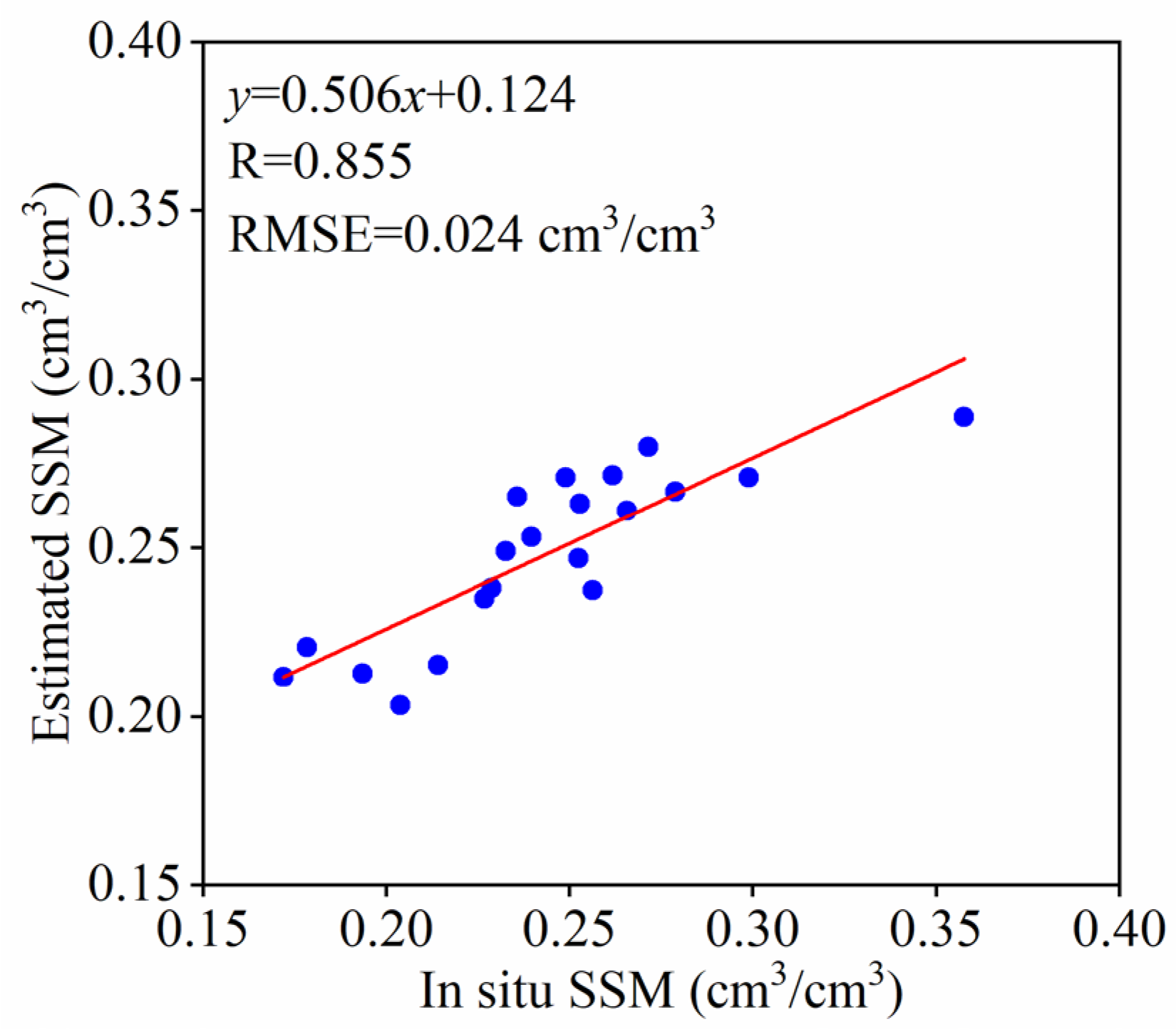
Figure 6 shows the results of the validation of the inversion model of SSM in vegetated areas. As can be seen from Figure 6, the validation accuracy for SSM in vegetation cover and the in situ SSM is high (R = 0.855; RMSE = 0.024 cm3/cm3) and uniformly distributed on both sides of a 1:1 straight line, which indicates that it is feasible and accurate to utilize the joint inversion of SSM using the WCM and the RBF neural network model in vegetated areas, which is in line with the results of a previous study [26]. Meanwhile, adding the NDVI to the input layer of the RBF neural network model can improve the accuracy of the inversion.
The backscattering of bare soil and the RBF neural network model were used to construct an inversion model of SSM in bare soil. The input data of the RBF neural network model contained the backscattering of bare soil in VV polarization (σbare_VV), the backscattering of bare soil in VH polarization (σbare_VH), the difference in VV polarization and VV polarization (σbare_VV–σbare_VH), and θ, and the output data was the SSM.
Figure 7 shows the validation results of the SSM inversion model in bare soil. As can be seen from Figure 7, it is feasible to use the RBF neural network model to construct an inversion model of SSM in bare soil, and the inversion accuracy is high (R = 0.796; RMSE = 0.029 cm3/cm3) and uniformly distributed on both sides of the 1:1 line, which is in line with the results of a previous study [25]. Compared with the Shi model and Oh model, the RBF neural network model has a simple structure and fewer input parameters, which is superior to the accuracy of the inversion model of VV-polarized SSM established by Wang et al. [36] (R = 0.653; RMSE = 0.0832 cm3/cm3).

3.2.2. Linear Model Inversion of Surface Soil Moisture

Figure 8 shows the VV-polarized linear model and validation results. Soil backscattering was obtained by removing the effect of vegetation using the WCM. The SSM inversion model was established using soil backscattering in VV polarization and in situ SSM. The SSM inversion model was established at 58 points, and the model accuracy was validated at 47 points. The linear regression model is feasible and has high accuracy (R = 0.752; RMSE = 0.058 cm3/cm3). The small inversion values of the model may be caused by a single parameter in the linear model, which does not fully consider the influence of surface roughness.
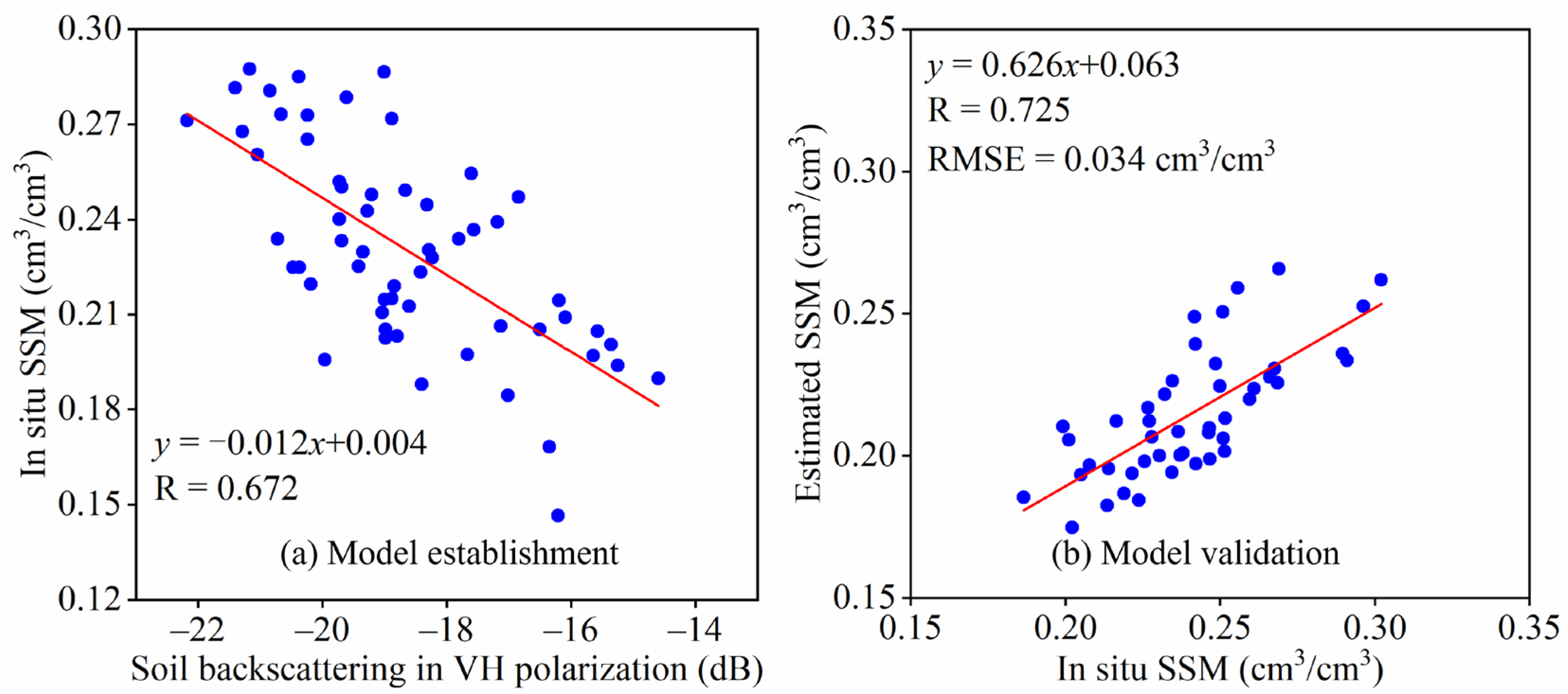
Figure 9 shows the VH-polarized linear model and validation results. Soil backscattering in VH polarization was obtained by removing the effect of vegetation using the WCM, and the SSM inversion model was established using soil backscattering and in situ SSM. In total, 58 points were selected to establish the SSM inversion model, and 47 points were validated for model accuracy. The linear regression model is feasible and has high accuracy (R = 0.725; RMSE = 0.034 cm3/cm3). The small value of the estimated SSM may be caused by the linear model introducing a single covariate and not fully considering the influence of surface roughness. It is better than the accuracy of the VH polarization inversion of SSM established by Wang et al. [36] (R = 0.491; RMSE = 0.0979 cm3/cm3).
In vegetated areas, the RBF neural network model improved by 0.103, and the RMSE decreased by 0.034 cm3/cm3 relative to the VV-polarization-based linear regression model’s R. The RMSE decreased by 0.01 cm3/cm3 relative to the VH-polarization-based linear regression model’s R. In bare soil, the RBF neural network model increased the R by 0.044 and decreased the RMSE by 0.029 cm3/cm3 relative to the linear regression model based on VV polarization and increased the R by 0.071 and decreased the RMSE by 0.005 cm3/cm3 relative to the linear regression model based on VH polarization. The above analyses indicate that the RBF neural network model in the inverse model of SSM has better accuracy relative to the linear model, which is probably due to the introduction of more surface parameters into the RBF neural network model and the fact that the RBF neural network model is more accurate and more precise. This may be due to the fact that the introduction of more surface parameters to the model can better characterize soil backscattering.

4. Summary and Conclusions

In this study, by using WCM to remove the influence of vegetation on the inversion of SSM, it was found that the VWC calculated by different polarization methods and different data sources leads to differences in the contribution of vegetation to total backscattering. Specifically, in the VV polarization mode, the results of NDVI_Sentinel-2 and NDWI_Sentinel-2 for vegetation impact removal are different. When NDVI_Sentinel-2 was used to remove the effects of vegetation, the average contribution of vegetation to the total backscattering in VV polarization was 0.9 dB. When NDWI_Sentinel-2 was used to remove the effects of vegetation, the value was only 0.053 dB. Similarly, the effects of NDVI_Landsat-8 and NDWI_Landsat-8 on the impact of vegetation removal were different in VV polarization. When NDVI_Landsat-8 was selected as the parameter to calculate the VWC, the average contribution of vegetation to the total backscattering in VV polarization was 1.29 dB. When NDWI_Landsat-8 was used to remove vegetation effects, the value dropped to 0.115 dB. In VH polarization, the results of removing vegetation with NDVI_Sentinel-2 and NDWI_Sentinel-2 were different. When NDVI_Sentinel-2 was used to remove the effect of vegetation, the average contribution of vegetation to the total backscattering in VH polarization was 1.59 dB. When NDWI_Sentinel-2 was used to remove the effects of vegetation, the value was 0.094 dB. Similarly, in VH polarization, the results of removing vegetation influence with NDVI_Landsat-8 and NDWI_Landsat-8 were also different. When NDVI_Landsat-8 was selected, the average contribution of vegetation to the total backscattering in VH polarization was 2.26 dB. When NDWI_Landsat-8 was used to remove the influence of vegetation, the value was 0.21 dB. By exploring the reasons for these differences, we can make the following conclusions. First, the sensitivity of different polarization modes to vegetation and soil is different. Compared with VH polarization, VV polarization is more sensitive to SSM and contains more comprehensive soil information. Secondly, the calculation of VWC parameters and the selection of data sources may also have an impact on the results. The NDVI and NDWI calculated with the Sentinel-2 and Landsat-8 images used in this study showed significant differences in removing the impact of vegetation.
  • For VV and VH polarization, substituting the VWC calculated by NDVI into the WCM to remove the effect of the vegetation layer is better than NDWI; substituting the VWC calculated by NDVI_Landsat-8 into the WCM to remove the effect of the vegetation layer is better than using NDVI_Sentinel-2.
  • In vegetated areas, the inversion accuracy of the RBF neural network model was high (R = 0.855; RMSE = 0.024 cm3/cm3). Compared with the linear regression model in VV polarization, the R of the RBF neural network model increased by 0.103, and the RMSE decreased by 0.034 cm3/cm3. Compared with the linear regression model in VH polarization, the R of the RBF neural network model increased by 0.13, and the RMSE decreased by 0.01 cm3/cm3.
  • In bare soil, the inversion accuracy of the RBF neural network model is high (R = 0.796; RMSE = 0.029 cm3/cm3). Compared with the linear regression model in VV polarization, the R of the RBF neural network model increased by 0.044, and the RMSE decreased by 0.029 cm3/cm3. Compared with the linear regression model in VH polarization, the R of the RBF neural network model increased by 0.071, and the RMSE decreased by 0.005 cm3/cm3.

Author Contributions

Methodology, R.L.; Formal analysis, Z.W. and H.C.; Data curation, F.W. and D.H.; Funding acquisition, B.Z.; Project administration, Y.L.; Writing—review & editing, R.H. All authors have read and agreed to the published version of the manuscript.

Funding

This research was funded by the National Key Research and Development Program of China (No. 2022YFD1900500), the National Key Research and Development Program of China (No. 2023YFD1900801-02), the Chinese National Science Fund (No. 52130906), and the Independent Research Project of the State Key Laboratory of Simulation and Regulation of Water Cycle in River Basin (No. SKL2022TS13).

Institutional Review Board Statement

Not applicable.

Informed Consent Statement

Not applicable.

Data Availability Statement

The data presented in this study are available on request from the first author. The data are not publicly available due to privacy.

Acknowledgments

We would like to thank the anonymous reviewers for their long-term guidance and constructive comments. Moreover, we are grateful to the European Space Agency (ESA) and the United States Geological Survey (USGS), who provided remote sensing images for free.

Conflicts of Interest

The authors declare no conflicts of interest.

References

  1. Nguyen, H.H.; Cho, S.; Choi, M. Spatial soil moisture estimation in agro-pastoral transitional zone based on synergistic use of SAR and optical-thermal satellite images. Agric. For. Meteorol. 2022, 312, 108719. [Google Scholar] [CrossRef]
  2. Dorigo, W.; Wagner, W.; Albergel, C.; Albrecht, F.; Balsamo, G.; Brocca, L.; Chung, D.; Ertl, M.; Forkel, M.; Gruber, A.; et al. ESA CCI Soil Moisture for improved Earth system understanding: State-of-the art and future directions. Remote Sens. Environ. 2017, 203, 185–215. [Google Scholar] [CrossRef]
  3. Petropoulos, G.; Srivastava, P.; Piles, M.; Pearson, S. Earth Observation-Based Operational Estimation of Soil Moisture and Evapotranspiration for Agricultural Crops in Support of Sustainable Water Management. Sustainability 2018, 10, 181. [Google Scholar] [CrossRef]
  4. Abowarda, A.S.; Bai, L.; Zhang, C.; Long, D.; Li, X.; Huang, Q.; Sun, Z. Generating surface soil moisture at 30 m spatial resolution using both data fusion and machine learning toward better water resources management at the field scale. Remote Sens. Environ. 2021, 255, 112301. [Google Scholar] [CrossRef]
  5. Bogena, H.R.; Huisman, J.A.; Güntner, A.; Hübner, C.; Kusche, J.; Jonard, F.; Vey, S.; Vereecken, H. Emerging methods for noninvasive sensing of soil moisture dynamics from field to catchment scale: A review. WIREs Water 2015, 2, 635–647. [Google Scholar] [CrossRef]
  6. Long, D.; Bai, L.; Yan, L.; Zhang, C.; Yang, W.; Lei, H.; Quan, J.; Meng, X.; Shi, C. Generation of spatially complete and daily continuous surface soil moisture of high spatial resolution. Remote Sens. Environ. 2019, 233, 111364. [Google Scholar] [CrossRef]
  7. Whyte, A.; Ferentinos, K.P.; Petropoulos, G.P. A new synergistic approach for monitoring wetlands using Sentinels -1 and 2 data with object-based machine learning algorithms. Environ. Modell. Softw. 2018, 104, 40–54. [Google Scholar] [CrossRef]
  8. Liu, Z.; Todini, E. Towards a comprehensive physically-based rainfall-runoff model. Hydrol. Earth Syst. Sci. 2002, 6, 859–881. [Google Scholar] [CrossRef]
  9. Ochsner, T.E.; Cosh, M.H.; Cuenca, R.H.; Dorigo, W.A.; Draper, C.S.; Hagimoto, Y.; Kerr, Y.H.; Larson, K.M.; Njoku, E.G.; Small, E.E.; et al. State of the Art in Large-Scale Soil Moisture Monitoring. Soil Sci. Soc. Am. J. 2013, 77, 1888–1919. [Google Scholar] [CrossRef]
  10. Lu, L.; Luo, G.-P.; Wang, J.-Y. Development of an ATI-NDVI method for estimation of soil moisture from MODIS data. Int. J. Remote Sens. 2014, 35, 3797–3815. [Google Scholar] [CrossRef]
  11. Kang, J.; Jin, R.; Li, X.; Ma, C.; Qin, J.; Zhang, Y. High spatio-temporal resolution mapping of soil moisture by integrating wireless sensor network observations and MODIS apparent thermal inertia in the Babao River Basin, China. Remote Sens. Environ. 2017, 191, 232–245. [Google Scholar] [CrossRef]
  12. Sezen, S.M.; Yazar, A.; Daşgan, Y.; Yucel, S.; Akyıldız, A.; Tekin, S.; Akhoundnejad, Y. Evaluation of crop water stress index (CWSI) for red pepper with drip and furrow irrigation under varying irrigation regimes. Agric. Water Manag. 2014, 143, 59–70. [Google Scholar] [CrossRef]
  13. Lin, R.; Chen, H.; Wei, Z.; Li, Y.; Zhang, B.; Sun, H.; Cheng, M. Improved Surface Soil Moisture Estimation Model in Semi-Arid Regions Using the Vegetation Red-Edge Band Sensitive to Plant Growth. Atmosphere 2022, 13, 930. [Google Scholar] [CrossRef]
  14. Oh, Y.; Sarabandi, K.; Ulaby, F.T. An empirical model and an inversion technique for radar scattering from bare soil surfaces. IEEE Trans. Geosci. Remote Sens. 1992, 30, 370–381. [Google Scholar] [CrossRef]
  15. Fung, A.K.; Li, Z.; Chen, K.S. Backscattering from a randomly rough dielectric surface. IEEE Trans. Geosci. Remote Sens. 1992, 30, 356–369. [Google Scholar] [CrossRef]
  16. Dubois, P.C.; van Zyl, J.; Engman, T. Measuring soil moisture with imaging radars. IEEE Trans. Geosci. Remote Sens. 1995, 33, 915–926. [Google Scholar] [CrossRef]
  17. Chen, K.S.; Tzong-Dar, W.; Leung, T.; Qin, L.; Jiancheng, S.; Fung, A.K. Emission of rough surfaces calculated by the integral equation method with comparison to three-dimensional moment method simulations. IEEE Trans. Geosci. Remote Sens. 2003, 41, 90–101. [Google Scholar] [CrossRef]
  18. Ulaby, F.T.; Sarabandi, K.; McDonald, K.; Whitt, M.; Dobson, M.C. Michigan microwave canopy scattering model. Int. J. Remote Sens. 2007, 11, 1223–1253. [Google Scholar] [CrossRef]
  19. Attema, E.P.W.; Ulaby, F.T. Vegetation modeled as a water cloud. Radio Sci. 1978, 13, 357–364. [Google Scholar] [CrossRef]
  20. Lv, A.; Zhang, Z.; Zhu, H. A Neural-Network Based Spatial Resolution Downscaling Method for Soil Moisture: Case Study of Qinghai Province. Remote Sens. 2021, 13, 1583. [Google Scholar] [CrossRef]
  21. Ali, I.; Greifeneder, F.; Stamenkovic, J.; Neumann, M.; Notarnicola, C. Review of Machine Learning Approaches for Biomass and Soil Moisture Retrievals from Remote Sensing Data. Remote Sens. 2015, 7, 16398–16421. [Google Scholar] [CrossRef]
  22. Sheng, Z.B.; Tong, X.R. The Application of RBF Neural Networks in Curve Fitting. Adv. Mater. Res. 2012, 490–495, 688–692. [Google Scholar] [CrossRef]
  23. Lu, Z.; Meyer, D.J. Study of high SAR backscattering caused by an increase of soil moisture over a sparsely vegetated area: Implications for characteristics of backscattering. Int. J. Remote Sens. 2010, 23, 1063–1074. [Google Scholar] [CrossRef]
  24. Lievens, H.; Verhoest, N.E.C. On the Retrieval of Soil Moisture in Wheat Fields From L-Band SAR Based on Water Cloud Modeling, the IEM, and Effective Roughness Parameters. IEEE Geosci. Remote Sens. Lett. 2011, 8, 740–744. [Google Scholar] [CrossRef]
  25. Bao, Y.; Lin, L.; Wu, S.; Kwal Deng, K.A.; Petropoulos, G.P. Surface soil moisture retrievals over partially vegetated areas from the synergy of Sentinel-1 and Landsat 8 data using a modified water-cloud model. Int. J. Appl. Earth Obs. Geoinf. 2018, 72, 76–85. [Google Scholar] [CrossRef]
  26. Chen, K.; Cao, X.; Shen, F.; Ge, Y. An Improved Method of Soil Moisture Retrieval Using Multi-Frequency SNR Data. Remote Sens. 2021, 13, 3725. [Google Scholar] [CrossRef]
  27. Han, X.; Wei, Z.; Zhang, B.; Li, Y.; Du, T.; Chen, H. Crop evapotranspiration prediction by considering dynamic change of crop coefficient and the precipitation effect in back-propagation neural network model. J. Hydrol. 2021, 596, 126104. [Google Scholar] [CrossRef]
  28. Lee, J.S.; Jurkevich, L.; Dewaele, P.; Wambacq, P.; Oosterlinck, A. Speckle filtering of synthetic aperture radar images: A review. Remote Sens. Rev. 1994, 8, 313–340. [Google Scholar] [CrossRef]
  29. Hosseini, M.; McNairn, H.; Mitchell, S.; Robertson, L.D.; Davidson, A.; Ahmadian, N.; Bhattacharya, A.; Borg, E.; Conrad, C.; Dabrowska-Zielinska, K.; et al. A Comparison between Support Vector Machine and Water Cloud Model for Estimating Crop Leaf Area Index. Remote Sens. 2021, 13, 1348. [Google Scholar] [CrossRef]
  30. Ouaadi, N.; Jarlan, L.; Ezzahar, J.; Zribi, M.; Khabba, S.; Bouras, E.; Bousbih, S.; Frison, P.-L. Monitoring of wheat crops using the backscattering coefficient and the interferometric coherence derived from Sentinel-1 in semi-arid areas. Remote Sens. Environ. 2020, 251, 112050. [Google Scholar] [CrossRef]
  31. Kumar, K.; Suryanarayana Rao, H.P.; Arora, M.K. Study of water cloud model vegetation descriptors in estimating soil moisture in Solani catchment. Hydrol. Processes 2015, 29, 2137–2148. [Google Scholar] [CrossRef]
  32. Bindlish, R.; Barros, A.P. Parameterization of vegetation backscatter in radar-based, soil moisture estimation. Remote Sens. Environ. 2001, 76, 130–137. [Google Scholar] [CrossRef]
  33. Jackson, T.; Le Vine, D.; Hsu, A.; Oldak, A.; Starks, P.; Swift, C.; Isham, J.; Haken, M. Soil moisture mapping at regional scales using microwave radiometry: The Southern great plains hydrology experiment. IEEE Trans. Geosci. Remote Sens. 1999, 37, 2136–2151. [Google Scholar] [CrossRef]
  34. Jackson, T. Vegetation water content mapping using Landsat data derived normalized difference water index for corn and soybeans. Remote Sens. Environ. 2004, 92, 475–482. [Google Scholar] [CrossRef]
  35. Changhua, C.; Jun, T.; Jiankang, Y.; Fei, Z.; Jin, Y. Prediction for soil moisture in tobacco fields based on PCA and RBF neural network. Trans. Chin. Soc. Agric. Eng. 2010, 26, 85–90. [Google Scholar] [CrossRef]
  36. Wang, E.-l.; Wang, J.; Han, J.; Chen, L.; Xiang, J.; He, B.; Chen, J. Baseed on Sentinel-1 and Sentinel-2 Synergistic Inversion of Surface Soil Moisture in Arid Areas-A case study of the Middle and Lower Reaches of Golmud River. J. Salt Lake Res. 2022, 30, 16–24. [Google Scholar] [CrossRef]
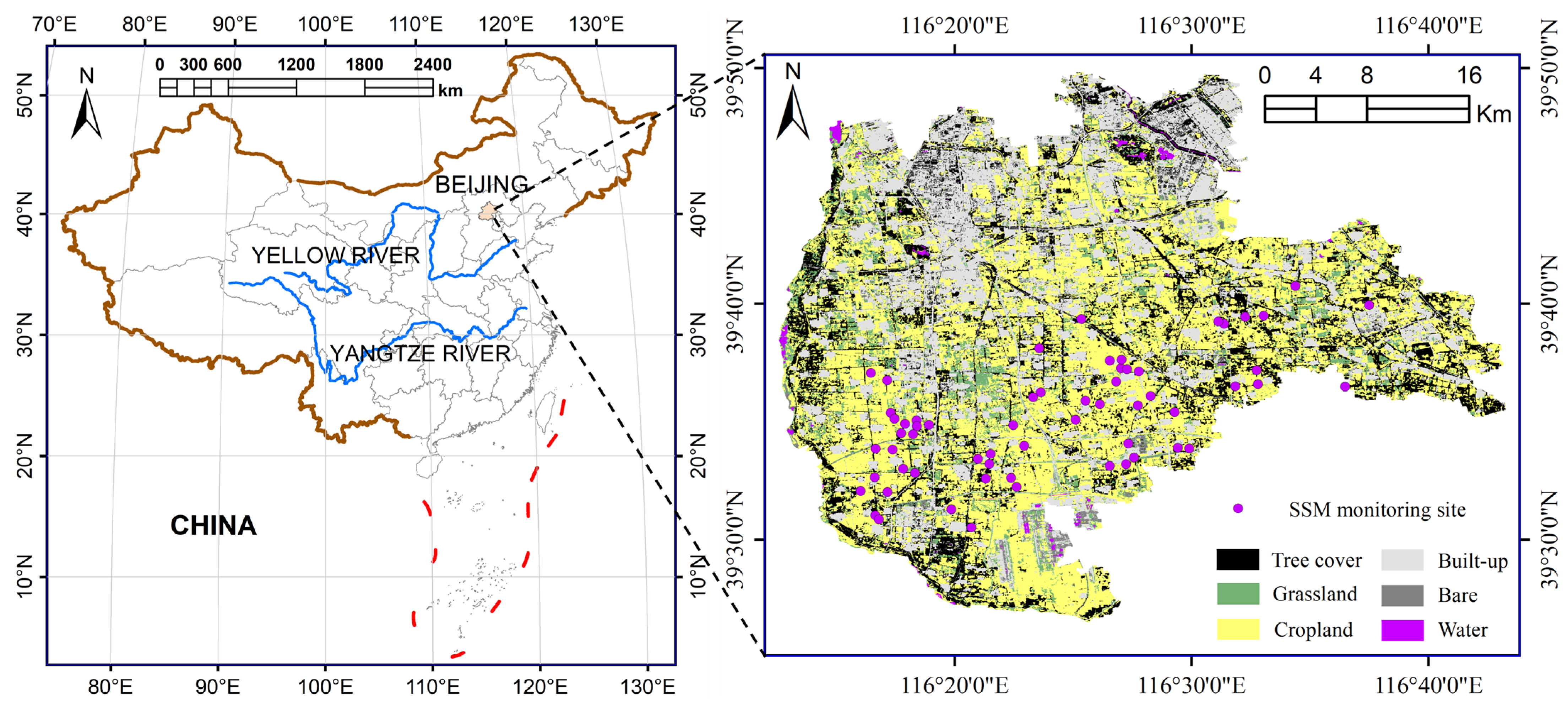
Figure 1. Geographical location of Daxing District, Beijing, China.
Atmosphere 15 00647 g001
Figure 2. Results of NDVI removal of vegetation backscattering calculated from different data sources in VV polarization: (a) Sentinel-2; (b) Landsat-8.
Atmosphere 15 00647 g002
Figure 3. Results of NDWI removal of vegetation backscattering calculated from different data sources in VV polarization: (a) Sentinel-2; (b) Landsat-8.
Atmosphere 15 00647 g003
Figure 4. Results of NDVI removal of vegetation backscattering calculated from different data sources in VH polarization: (a) Sentinel-2; (b) Landsat-8.
Atmosphere 15 00647 g004
Figure 5. Comparison of effects of VH polarization and NDWI removal from different data sources: (a) Sentinel-2; (b) Landsat-8.
Atmosphere 15 00647 g005
Figure 6. Validation of inversion model of SSM in vegetated areas.
Atmosphere 15 00647 g006
Figure 7. Validation of inversion model of SSM in bare soil.
Atmosphere 15 00647 g007
Figure 8. Establishment and validation of VV polarization linear model: (a) Model establishment; (b) Model validation.
Atmosphere 15 00647 g008
Figure 9. Establishment and validation of VH polarization linear model: (a) Model establishment; (b) Model validation.
Atmosphere 15 00647 g009
Table 1. Data acquisition date.
DataDate
Sentinel-122 July 2021, 3 August 2021, 15 August 2021, 27 August 2021, 8 September 2021, 20 September 2021, 2 October 2021, 26 October 2021
Sentinel-22 August 2021, 5 August 2021, 17 August 2021, 27 August 2021, 9 September 2021, 21 September 2021, 26 October 2021, 22 July 2020, 3 August 2020, 7 September 2020, 1 October 2020
Landsat-86 August 2021, 7 September 2021
SSM22 July 2021, 3 August 2021, 14 August 2021, 27 August 2021, 8 September 2021, 2 October 2021, 26 October 2021
Disclaimer/Publisher’s Note: The statements, opinions and data contained in all publications are solely those of the individual author(s) and contributor(s) and not of MDPI and/or the editor(s). MDPI and/or the editor(s) disclaim responsibility for any injury to people or property resulting from any ideas, methods, instructions or products referred to in the content.