Cloud Top Height Retrieval from FY-4A Data: A Residual Module and Genetic Algorithm Approach

Abstract

This paper proposes a ResGA-Net algorithm for cloud top height (CTH) retrieval using FY-4A satellite data. The algorithm utilizes genetic algorithms for data selection and employs a residual module-based neural network for modeling. It takes the spectral channel data from the FY-4A satellite as input features and uses CTH extracted from ground-based millimeter-wave cloud radar reflectivity as the target. By combining the large observation scale of the FY-4A satellite and the high accuracy of ground-based cloud radar observations, the model can generate satellite CTH products with higher precision. To validate the effectiveness of the algorithm, experiments were conducted using data from the Beijing area spanning from January 2020 to January 2022. The experimental results show that the metrics of the proposed ResGA-Net outperform those of various contrastive algorithms, and compared to the original FY-4A CTH product, the RMSE and MAE have decreased by 37.89% and 34.77%, while the PCC and SRCC have increased by 11.17% and 9.47%, respectively, demonstrating the superiority of the proposed method presented in this paper.

1. Introduction

Clouds are vital for the Earth’s water cycle, as water evaporates from rivers, lakes, oceans, soil, and plants into the air, becoming water vapor that can form clouds or precipitation after entering the atmosphere [1]. Today, the impact of weather on human life is not limited to agriculture and transportation but also greatly affects social and economic development. Additionally, the frequent occurrence of global warming and extreme weather events has made people increasingly dependent on accurate weather forecasts.

Cloud top height (CTH, usually in meters) is a fundamental property of clouds, which serves not only as a significant aspect of meteorological forecasting and atmospheric science research but also as a vital indicator of weather changes. Furthermore, CTH not only aids in the generation of other cloud product data, such as cloud thickness [2] and surface radiation beneath the clouds [3], but also contributes to the generation of other data used in meteorological research, including particle phase in clouds [4], water vapor content, and precipitation estimation [5,6]. The variability in CTH also holds significant implications for daily life and industrial activities, such as impacting aircraft flight paths and speeds [7]. Therefore, the accurate retrieval of CTH holds crucial significance.

CTH data are mainly obtained through observation methods such as cloud radar and meteorological satellites. Cloud radar can provide relatively accurate local CTH data, but it is limited by spatial range and detection conditions, making it difficult to acquire continuous spatial data. On the other hand, satellite scanning has the advantages of large coverage, high spatiotemporal resolution, and being less affected by natural or geographical conditions, but the accuracy of CTH data is relatively poor [8,9].

Currently, there are many classical satellite-based CTH retrieval methods, such as the channel brightness temperature method [10,11], multi-satellite joint observation method [12,13], split window method [14,15,16,17], carbon dioxide layering method [18,19], and machine learning methods [20,21,22].

CTH exhibits an almost linear relationship with cloud top temperature and cloud top pressure. As the CTH increases, the cloud top temperature and cloud top pressure decrease. Conversely, as the CTH decreases, the cloud top temperature and cloud top pressure increase. Single and multi-channel brightness temperature methods leverage this principle by, first, obtaining radiance from sensors to convert radiance values into cloud top temperature and cloud top pressure, and, finally, convert them into CTH. In 2022, Duan et al. used 11.2 μm channel data from geostationary meteorological satellites and temperature–pressure layer data from ERA5 reanalysis to retrieve CTH, successfully retrieving the CTH of some high-level clouds [10]. In 2016, Gu et al. used a fast radiative transfer model to simulate channel brightness temperatures and found that, when clouds exist at multiple heights, the brightness temperature of the channel depends on the highest cloud layer, especially for thin and low clouds [11].

Multi-satellite joint observation refers to the simultaneous observation of the same cloud by two or more meteorological satellites from different angles and positions. In 2020, Lee et al. used Himawari-8 and FY2E geostationary meteorological satellites to observe the CTH and proposed the GEO-CTH algorithm based on parallax estimation. This algorithm involves four steps: image remapping, image matching, CTH calculation, and quality control, resulting in reliable CTH estimates [12]. In 2021, Li et al. studied FY-4A and Himawari-8 geostationary meteorological satellites and found that, although data errors and missing data issues limit the reliability of joint observation from geostationary satellites, FY-4A and Himawari-8 data exhibit good consistency and can be used for dual-satellite joint observation [13].

The split window method involves utilizing two adjacent channels within the atmospheric window of 8~14 μm (typically, 10.5~11.5 μm and 11.5~12.5 μm), whereby cloud radiance and background radiance from each channel are input into the corresponding split window method formula to calculate the CTH [14]. In 2019, Y. B. Liang and colleagues established a split window histograms method using Himawari-8’s AHI observation data. The results of CTH retrieval for semi-transparent clouds showed a high level of consistency with the CloudSat dataset. Their research also indicated that the underlying surface type did not have a significant impact on the retrieval results [15]. In 2010, Hamada and his team discovered that, by using the infrared brightness temperature at 10.8 μm and the difference between the infrared brightness temperatures at 10.8 μm and 12 μm, they could estimate the CTH and visible optical thickness of some high-level clouds. The split window method allowed them to obtain CTH data at an hourly resolution, and this data was reliable in regions other than areas with a high satellite zenith angle [16]. In 2017, Noriyuki et al. proposed a split window method using infrared observations on geostationary satellites to retrieve the CTH, applied it to the CALIPSO and CloudSat satellites, and established a practical CTH lookup table, effectively correcting errors in cirrus cloud height [17].

The carbon dioxide (CO₂) layering technique utilizes the absorption characteristics of CO₂ in the atmosphere. As the wavelength increases from 13.3 to 15 μm, the atmosphere becomes opaquer. This allows radiation from these bands to sensitively reflect different layers in the atmosphere [18]. The CTH product from the China Meteorological Administration’s FY-4A meteorological geostationary satellite is obtained through the FCTHA algorithm, which incorporates the advantages of the infrared split window and CO₂ layering methods. The retrieved CTH product shows high consistency when compared to similar international products [19].

Machine learning-based meteorological algorithms are also evolving and providing new solutions for retrieving and forecasting meteorological parameters. In 2022, Yu et al. investigated whether building models separately based on cloud type for cloud height retrieval is better than not classifying clouds. They used two ensemble learning models to retrieve cloud heights: the first model retrieved the height for eight cloud types separately, while the second model retrieved heights for all the clouds uniformly. The results showed that the first ensemble learning model performed better [20]. In 2022, Dong et al. proposed a CTH retrieval algorithm based on XGBoost. This algorithm utilizes multi-channel radiance data and calculates the input parameters for the model based on cloud phase; texture; local brightness temperature changes; and geographical factors such as latitude, solar zenith angle, and satellite zenith angle to reduce the impact of the land–sea position and other geographical factors on CTH retrieval [21]. In 2021, Rysman et al. achieved good results using a machine learning-based approach that combined neural networks and gradient boosting methods, using satellite-observed brightness temperature data and auxiliary data such as temperature, relative humidity, etc., as inputs for retrieving CTH [22].

Although researchers have explored many methods for CTH retrieval, most of them have been limited to single observation devices or data sources. Nowadays, new devices like millimeter-wave cloud radars can provide high-precision CTH data. To our knowledge, there is currently no method that combines the use of geostationary meteorological satellites and millimeter-wave cloud radars for cloud top height retrieval. Different from the aforementioned methods, this paper proposes a CTH retrieval algorithm that combines genetic algorithms and residual networks, leveraging the advantages of the FY-4A satellite and ground-based cloud radar for CTH retrieval. The main contributions of this study are as follows:

(1) While FY-4A offers wide observation coverage, its secondary CTH data accuracy is relatively low, whereas ground-based cloud radar provides high accuracy but is limited by observation conditions. The algorithm leverages the advantages of both by using FY-4A’s multi-channel scanning data as the input and ground-based cloud radar data as the target value modeling.

(2) Considering that cloud radar has high sensitivity but is susceptible to noise, this method utilizes genetic algorithms for sample selection and machine learning algorithms for modeling, thereby generating high-precision CTH products.

2. Methodology

2.1. Overall Architecture

The proposed model in this study utilizes high-precision scanning data from ground-based cloud radars as labels. However, due to various uncontrollable factors, the dataset may contain some outliers or abnormal data samples, which can negatively impact the subsequent CTH retrieval work. Therefore, this paper combines genetic algorithms with the residual-enhanced neural network (residual-enhanced NN) to perform quality control on the sample dataset. This approach aims to filter out the exceptional samples. The model that combines genetic algorithms and the residual-enhanced NN is referred to as ResGA-Net in this paper. The structure diagram of the model is depicted in Figure 1.

The genetic algorithm (GA) mimics biological evolution by iteratively improving the dataset quality through selection, crossover, and mutation operations. Individuals with superior attributes are favored in each generation, leading to a gradual enhancement of the dataset quality. This process continues until convergence, resulting in a meticulously refined dataset.

The refined dataset is then fed into the residual-enhanced neural network (residual-enhanced NN), a robust neural network structure pivotal for both the training and prediction phases. During training, optimized data are put into the residual-enhanced NN, utilizing feedforward and feedback propagation and leveraging residual connections to capture features across various levels. The model progressively adjusts its parameters to fit the characteristics of the optimized data, thereby improving the performance in CTH retrieval tasks.

In the prediction phase, the test data are directly put into the residual-enhanced NN, and the CTH prediction results are obtained through forward propagation.

The ResGA-Net model innovatively combines the genetic algorithm and residual-enhanced NN modules. This collaboration offers significant advantages in CTH retrieval tasks by enhancing the dataset quality at the dataset level and enabling the residual-enhanced NN to train and predict using superior-quality data.

2.2. Genetic Algorithm Module

The genetic algorithm is an adaptive heuristic search algorithm based on population genetics inspired by the biological evolutionary process and reflecting Darwin’s theory of “survival of the fittest” [23]. It is widely used for solving optimization and search problems. Initially, a population of random solutions (chromosomes) is generated, each comprising various attributes (genes). Through crossover and mutation, chromosomes evolve into the next generation, fostering diversity. This iterative process aims to find optimal or approximate solutions to problems. The key components include chromosome encoding, population initialization, fitness function definition, and genetic operation design.

As an optimization method, genetic algorithms are widely employed in the field of machine learning for optimizing model parameters. Additionally, genetic algorithms have also been explored for sample selection, aiding in the extraction of the most representative samples or filtering out anomalous samples from large-scale datasets, thereby enhancing the training efficiency and model generalization capabilities. Aggarwal et al. utilized evolutionary computing methods to detect anomalies in high-dimensional problems [24]. The experimental results indicated that evolutionary computing achieved comparable performance to brute force detection while requiring less time and lower manpower costs. From the perspective of data mining applications, this research holds significant reference value. Tianhu Zhang et al. employed genetic algorithms and backpropagation neural networks (BPNNs) in the field of atmospheric temperature and humidity retrieval. They optimized the training sample data and identified abnormal data samples, thus establishing a more accurate neural network model for atmospheric temperature and humidity profile retrieval [25]. Both of these works verified the feasibility of using genetic algorithms and BPNNs for removing anomalous samples from datasets.

Data quality control can eliminate a large amount of anomalous data, but there may still be some outlier data samples in the dataset, which can affect the subsequent CTH retrieval work. The genetic algorithm, as an evolutionary algorithm based on the principles of evolution and genetics, possesses strong optimization capabilities. Meanwhile, the BP neural network method exhibits powerful nonlinear fitting capabilities. By combining the genetic algorithm and BP neural network to optimize the training data, it is possible to discard outlier samples that distort CTH measurements from millimeter-wave cloud radar, thereby improving the retrieval accuracy. The implementation steps are as follows:

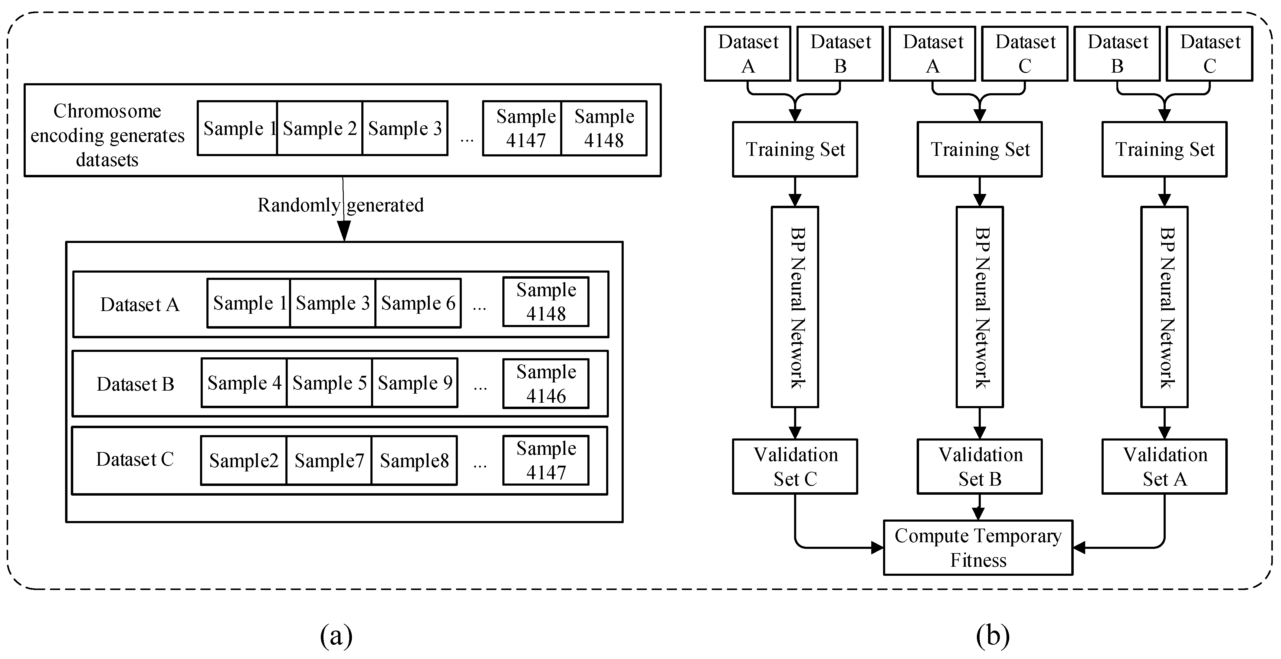
(1) Chromosome Encoding Design: As shown in Figure 2, chromosome encoding adopts the most commonly used binary coding scheme, where each gene of the chromosome is represented by 1 or 0. Here, each chromosome represents a solution to the sample optimization problem, with each gene in the chromosome representing a data sample. After the spatiotemporal matching and preliminary processing of the FY-4A geostationary meteorological satellite and the millimeter-wave cloud radar, 5185 data samples are selected for the genetic algorithm module of ResGA-Net. Therefore, the chromosome gene length is set to 5185 and is represented by 0 or 1. Here, 0 represents discarding the sample, while 1 represents retaining the sample. During the initialization of the population, considering the sample size, computational efficiency, and the final model results, 80% of the genes in the chromosome can be randomly set to 1, while the remaining 20% of the genes are set to 0. This setting can balance the sample size and computational efficiency to a certain extent while ensuring that the final model is trained and optimized with the retention of the most useful samples.

(2) Initialization of Population: The population size and the number of iterations can significantly impact the effectiveness and performance of the algorithm. It is generally recommended to have a population size ranging from 20 to 100 and the number of iterations between 100 and 500. Larger populations typically help maintain diversity in the solution space and enable faster exploration of the solution space. However, they also require more computational resources and time. Therefore, it is essential to make a reasonable choice based on the specific problem when applying genetic algorithms.

In this study, the genetic algorithm employs a population consisting of 51 chromosomes (51 being the setting for hyperparameters), and the population size remains unchanged after each iteration. Among these, 50 chromosomes are obtained through selection, crossover, and mutation operations, while 1 chromosome is preserved using an elitist retention strategy to retain the chromosome with the best fitness from the previous iteration. Each chromosome corresponds to a particular data sample selection.

(3) Fitness Calculation: In this study, a BP neural network is used to calculate the fitness of the genetic algorithm. To avoid the BP neural network getting trapped in local optima, the three-fold cross-validation method is employed, and a model is built for each fold. The specific steps are as follows: Firstly, based on the chromosome encoding, the corresponding data samples are selected to form a dataset. The dataset is then randomly divided into three sets. The diagram in Figure 3a illustrates the random generation of the fitness calculation data. Secondly, a BP neural network is constructed and trained, and the sum of squared errors (SSE) of the model on the validation set is calculated as the temporary fitness of the model. The diagram in Figure 3b illustrates the calculation of the temporary fitness. Lastly, the final fitness of all the chromosomes is calculated using the inverse formula, which can be expressed as Equation (1):

$$fitnes{s}_i=\frac{Max-x_i}{Max-Min}$$

(1)

where $Max$ represents the maximum SSE among all the chromosomes, $Min$ represents the minimum SSE of the chromosomes, and $x_i$ represents the SSE of the ith chromosome.

The BP neural network takes the FY-4A geostationary meteorological satellite’s Channel 09–14 spectral channel data as the input features and predicts the CTH as the output. During model training, the mean squared error (MSE) is used as the loss function, and the Adam optimization algorithm is employed for model optimization. The initial learning rate is set to 0.1, and a total of 2000 rounds of training are conducted. Early stopping is applied to prevent overfitting, where the number of data samples processed per round is half the length of the training set. A data shuffling strategy is implemented, and the learning rate will be half as high every 200 rounds.

(4) Selection: In this study, both roulette wheel selection and tournament selection operators are used during the selection step. Specifically, 15 chromosomes are generated using the roulette wheel selection operator, while 35 chromosomes are generated using the tournament selection operator. The roulette wheel selection operator randomly selects from five candidate chromosomes with equal probability, while the tournament selection operator chooses the chromosome with the highest fitness from the five candidate chromosomes.

(5) Crossover Operator: The multiple-point crossover operator is used in the crossover step of the genetic algorithm. Randomly selecting a parent chromosome, 1038 sets of 0/1 encoding groups are randomly generated within the parent and offspring chromosomes. Each set of 0/1 encoding groups has a 70% probability of gene exchange with the corresponding 0/1 encoding group at the same position in the parent chromosome (both encoding groups have an equal chance of being selected). The resulting offspring chromosome from the exchange is preserved as a new chromosome, replacing the original offspring chromosome.

(6) Mutation: The bit-flip mutation operator is used in the mutation step of the genetic algorithm. Within the chromosome, 1038 sets of 0/1 encoding groups are randomly generated, and each set has a 10% probability of undergoing mutation. The mutation swaps the encoding values within the 0/1 encoding group, resulting in a new chromosome.

(7) Elitism: The elitism strategy is employed in this study. The chromosome with the highest fitness is directly preserved in the next-generation population, avoiding disruption from crossover and mutation operations. This helps improve the convergence speed and global search capability of the algorithm.

The algorithmic process of using genetic algorithms for data selection is illustrated in Algorithm 1. After 500 rounds of iterations, the optimal chromosome obtained has the lowest SSE, indicating that the group of samples represented by this optimal chromosome can be considered as the filtered samples.

Algorithm 1: Genetic Algorithm for Data Selection.

Input: population size n, number of genes per chromosome m, maximum number of iterations maxIterations, probability of mutation mutationRate, probability of crossover crossoverRate Output: BestChromosome, the best solution found   1: Initialize a population with n chromosomes, each with m genes   2: for generation = 1 to MaxIterations do   3:    CalculateFitness()   4:    Selection()   5:    Crossover(CrossoverRate)   6:    Mutation(MutationRate)   7:    Elitism()   8: end for   9: Get the chromosome with the highest fitness   10: return BestChromosome

2.3. Residual-Enhanced NN

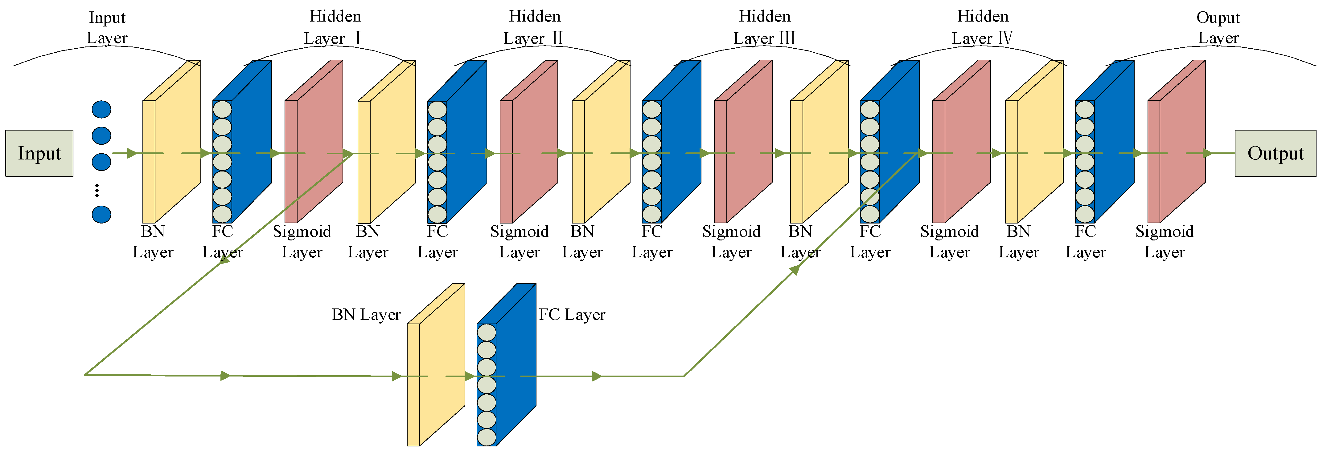
The entire network consists of six layers, including input and output layers, as well as four hidden layers. For neural network models, a shallow network lacks sufficient fitting capability, while a deep network can be challenging to train. Based on previous experience [26,27], four hidden layers were chosen as a balanced choice. By incorporating residual-like modules into feedforward neural networks, it becomes possible to combine the advantages of skip connections in residual networks, thereby enhancing the stability of the model. Driven by the integration of residual thinking, the network can not only mitigate the issue of “decreasing accuracy with increasing network depth” caused by gradient-related network degradation but also, to some extent, reduce problems like information loss and degradation [28]. We term this type of neural network, which embraces such fused residual-like structures, as the residual-enhanced NN, and its architectural diagram is depicted in Figure 4.

The residual-enhanced structure contains jump connections in a particular layer range. The jump links allow the feature maps in the first layer to reach the last layer directly. The mathematical expression of the residual-enhanced structure is as Equations (2) and (3):

$$y_l=h(x_l)+F(x_l,W_l)$$

(2)

$$x_{l+1}=f(y_l)$$

(3)

where $x_l$ is the input to the lth layer, $W_l$ is its weight, $y_l$ is the output, $h\left(\right)$ is a direct mapping, and $f\left(\right)$ is the activation function.

The residual block can be expressed as Equation (4). For a deeper layer $L$, its relationship with layer $l$ can be expressed as Equation (5):

$$x_{l+1}=x_l+F(x_l,W_l)$$

(4)

$$x_L=x_l+{\displaystyle \sum _{i=1}^{L-1}F(x_i,W_i)}$$

(5)

According to the chain rule for derivatives used in backpropagation, the gradient of the loss function $\epsilon$ with respect to $x_l$ can be expressed as Equation (6):

$$\begin{array}{l}\frac{\partial \epsilon }{\partial x_l}=\frac{\partial \epsilon }{\partial x_L}\frac{\partial x_L}{\partial x_l}\\ =\frac{\partial \epsilon }{\partial x_L}(1+\frac{\partial }{\partial x_l}{\displaystyle \sum _{i=l}^{L-1}F(x_i,W_i)})\\ =\frac{\partial \epsilon }{\partial x_L}+\frac{\partial \epsilon }{\partial x_L}\frac{\partial }{\partial x_l}{\displaystyle \sum _{i=l}^{L-1}F(x_i,W_i)}\end{array}$$

(6)

During the training of the neural network model, the input data enter the neural network through the input layer and are then processed by a BN (batch normalization) layer to ensure the consistency of data distribution and control gradient explosion and disappearance, thereby accelerating the network training speed [29]. Subsequently, the output of the BN layer is transmitted to the first hidden layer, where it undergoes processing by a fully connected linear layer. Afterward, it is activated by the sigmoid activation function. Sigmoid is one of the commonly used activation functions in neural networks. It introduces nonlinearity into the network, allowing it to learn and represent more complex patterns, and maps the output to a suitable bounded range. The activated data are then simultaneously passed to the second BN layer and a module resembling a residual structure. The data processed by the second BN layer are subsequently transferred to the third hidden layer, while the data processed by the residual-like module are transmitted to the fourth hidden layer. The activation process continues in this manner, with the data being propagated through each layer until reaching the output layer, which outputs the predicted data.

Next, the error between the predicted data and the true values is calculated. The weights and thresholds of the network’s layers are adjusted using the backpropagation algorithm based on this error. This process is repeated iteratively until the model converges or the predetermined number of iterations is reached.

3. Model Evaluation

3.1. Data Processing

3.1.1. Spatially and Temporally Matching of Satellite and Ground Observations

The Beijing Nanjiao Observatory is situated at a latitude of 39°48′ N and a longitude of 116°28′ E. By calculating the spherical distance between the centers of the 7,551,504 observation points within the 2748 × 2748 FY-4A geostationary meteorological satellite observation area and the coordinates of the Beijing Nanjiao Observatory, it was determined that the center coordinates of 405 rows and 1613 columns of observation points had the smallest spherical distance to the coordinates of the Beijing Nan-jiao Observatory, with an actual distance of only 1.968 km. Cloud clusters typically span tens to hundreds of kilometers, and the coverage area of each observation point of the FY-4A geostationary meteorological satellite is approximately 16 square kilometers. Therefore, the spectral channel values at this observation point on the FY-4A geostationary meteorological satellite effectively represent the radiation values above the Beijing Nanjiao Observatory.

The FY-4A geostationary meteorological satellite operates with an irregular full-disk observation cycle, while the millimeter-wave cloud radar provides CTH measurements over the station once per minute. By reading the “NOMObsTime” field in the level 1 data files of the FY-4A geostationary meteorological satellite, the observation time can be acquired. Subsequently, the CTH observed closest to the radar time is sought for matching. After validation, the observation time discrepancy is less than 30 s, indicating successful time synchronization.

3.1.2. Data Quality Control

The millimeter-wave cloud radar is an essential data source for the China Meteorological Administration. However, in the actual observation process, various abnormal situations may occur in the observed data due to various factors. Because the millimeter-wave transmitter and parabolic antenna are not protected by a cover and are in direct contact with the atmosphere, they can be affected by rain and snow during rainy and snowy weather, leading to the formation of water films or snow cover on the equipment’s surface, resulting in attenuation of the signal’s transmission and reception. This attenuation is particularly severe during rainy weather caused by deep convection and winter snowfall. Furthermore, the sensors of the millimeter-wave cloud radar can experience interference from sunlight when exposed for extended periods, especially during hot summers, leading to interference in the observed data, which can distort CTH measurements. Additionally, like conventional meteorological equipment, the millimeter-wave cloud radar can also be affected by various technical issues, such as power outages, short-duration surge currents, program anomalies, etc., resulting in missing data problems.

In the field of meteorology, data quality control is an essential step to ensure the quality and reliability of meteorological data. Before using the millimeter-wave cloud radar, it is necessary to perform data quality control to ensure data accuracy and consistency. By filtering out observation data that exhibit anomalies and distortions, data reliability can be effectively improved, ensuring the smooth progress of subsequent work. The data quality control rules used in this study provide preliminary quality control for CTH data, enhancing the reliability of the data. These rules primarily include cloud detection, the detection of abrupt changes in CTH data, and the smoothing of CTH data. By applying these steps to the data, noise and errors in the data can be reduced.

(1) Cloud Detection: During the data quality control process, cloud detection is an essential task. This study employs both FY-4A geostationary meteorological satellite cloud detection data and millimeter-wave cloud radar data to assess each data sample. If both data sources indicate the presence of clouds, the data sample is classified as “cloudy”; conversely, if both sources indicate the absence of clouds, the data sample is labeled as “clear”.

(2) Millimeter-Wave Cloud Radar Cloud Height Discontinuity Detection: CTH discontinuity detection, achieved through millimeter-wave cloud radar data, is a critical task within the data quality control process. Cloud morphology changes relatively slowly; if the CTH changes by over 1.5 km within 10 min, it is considered an anomaly in millimeter-wave cloud radar CTH data. Eleven CTH data samples, including five minutes before and after, are selected from the millimeter-wave cloud radar. By comparing the extreme values of these 11 data samples, if the extreme value difference is less than 1.5 km, the data sample is deemed normal. Conversely, if the difference exceeds 1.5 km, the data sample is considered anomalous and discarded from the dataset.

(3) Cloud Top Height Data Smoothing: Occasional inaccuracies exist in the observation times of the FY-4A geostationary meteorological satellite and millimeter-wave cloud radar data. CTH smoothing can mitigate this issue. Seven millimeter-wave cloud radar CTH data points, spanning three minutes before and after, are selected, and their average is taken as the true CTH value for that time.

3.2. Evaluation Metrics

This article uses four evaluation metrics to measure the experimental results, namely root mean squared error (RMSE), mean absolute error (MAE), Pearson correlation coefficient (PCC), and Spearman’s rank correlation coefficient (SRCC).

The Spearman’s rank correlation coefficient is a nonparametric statistical measure used to assess the monotonic relationship between two variables rather than a linear relationship. It is applicable to the relationship between the ranks (orderings) of data, without consideration for the absolute values of the data. The Spearman correlation coefficient helps us understand the tendency between two variables, indicating whether they change in similar patterns. Its expression is shown as Equation (7):

$$SRCC=1-\frac{6{\displaystyle \sum d_i^2}}{n(n^2-1)}$$

(7)

In statistics, the Pearson correlation coefficient (PCC) quantifies the correlation between two variables, X and Y, ranging from −1 to 1. Values close to these extremes suggest strong correlations, while values near 0 imply weak correlations. PCC is calculated as the covariance between the variables divided by the product of their standard deviations. The specific formula is shown in Equation (8):

$$\mathrm{r}=\frac{{\displaystyle \sum _{i=1}^n(X_i-\overline{X})(Y_i-\overline{Y})}}{\sqrt{{\displaystyle \sum _{i=1}^n{(X_i-\overline{X})}^2}}\sqrt{{\displaystyle \sum _{i=1}^n{(Y_i-\overline{Y})}^2}}}$$

(8)

RMSE (root mean square error) is a widely used metric for assessing regression model accuracy. It measures the disparity between predicted and observed values by taking the square root of the mean of squared differences. MAE (mean absolute error), on the other hand, computes the average absolute differences between observations and the mean value. MAE provides a precise representation of the prediction error magnitude, avoiding the issue of error cancellation, and its formula is shown as Equations (9) and (10):

$$RMSE=\sqrt{\frac{1}{n}{\displaystyle \sum _{i=1}^n{(Y_i-{\widehat{Y}}_i)}^2}}$$

(9)

$$MAE=\frac{1}{n}{\displaystyle \sum _{i=1}^n|Y_i-{\widehat{Y}}_i|}$$

(10)

In Equations (7) and (8), $n$ represents the total number of samples involved in the training, d represents the difference in ranks for each pair, and $\overline{X}$ and $\overline{Y}$ represent the sample means of variables X and Y, respectively. In Equations (9) and (10), ${\widehat{Y}}_i$ represents the predicted value of the ith sample.

3.3. Results and Analysis

This study takes data from January 2020 to January 2022 as an example. After spatiotemporal matching and data quality control of ground-based cloud radar and geostationary meteorological satellite data, a total of 6481 data samples are obtained. From these samples, 20% (1296 samples in total) are randomly selected as test samples, and all CTH retrieval models are tested on this set of test samples to obtain fair results. The remaining 5185 samples are used for training ResGA-Net and other CTH retrieval models. For ResGA-Net, 4147 data samples were selected through its GA module for subsequent modeling.

Upon computation, the root mean square error (RMSE), mean absolute error (MAE), Pearson correlation coefficient, and Spearman’s rank correlation coefficient for both the ResGA-Net model and the FY-4A CTH product are presented in

Table 1. Comparison of various algorithms and their indicator data.

Algorithm/Evaluation Metric	RMSE (m)	MAE (m)	PCC	SRCC
FY-4A CTH	1814.0	1406.8	0.752	0.760
LightGBM	1648.2	1287.7	0.778	0.765
Random Forest	1524.6	1193.5	0.795	0.746
CatBoost	1475.9	1177.2	0.801	0.778
SVR_rbf	1456.1	1091.8	0.808	0.792
ANN	1332.6	1072.4	0.814	0.806
ResGA-Net (ours)	1126.5	917.6	0.836	0.832

. From the table, it can be observed that the RMSE and MAE values for the results obtained using the ResGA-Net retrieval are reduced by 37.89% and 34.77%, respectively, compared to the original FY-4A product. Furthermore, the Pearson correlation coefficient reaches 0.836, and the Spearman’s rank correlation coefficient reaches 0.832, increased by 11.17% and 9.47%, respectively.

Additionally, this paper compares the effectiveness of machine learning algorithms such as Random Forest, LightGBM, CatBoost, SVR (rbf), and ANN in CTH retrieval, as shown in Table 1. One can see that, while the results of Random Forest, LightGBM, CatBoost, SVR (rbf), and ANN are all superior to the CTH data from the FY-4A secondary product, the ResGA-Net proposed in this paper outperforms them significantly in all metrics.

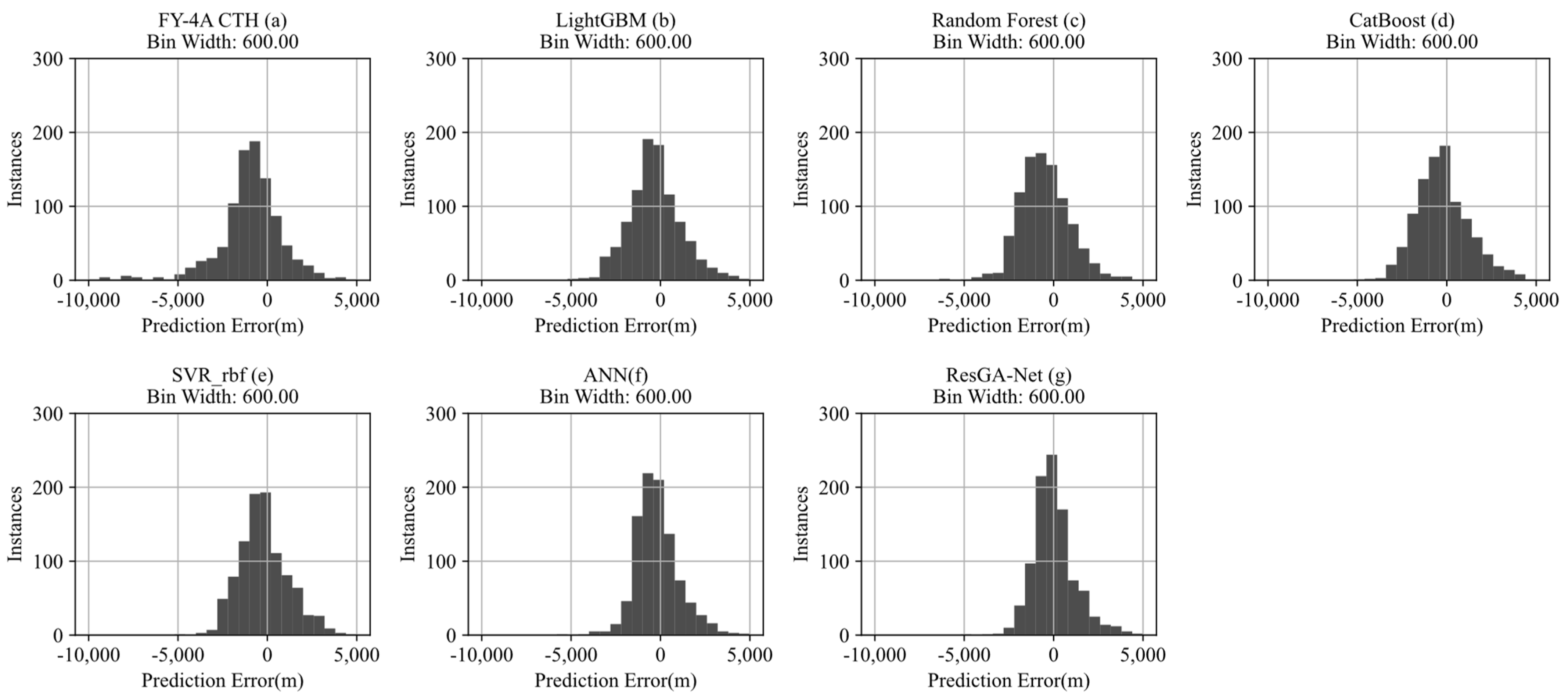
The scatter plot in Figure 5 illustrates the experimental results of the original FY-4A product compared to those obtained using the ResGA-Net algorithm and the aforementioned machine learning algorithms. The horizontal axis represents the predictions of each algorithm, while the vertical axis represents the CTH data from ground-based cloud radar. Each point in the plot that is closer to the centerline (where the centerline represents y = x) indicates that the model’s predictions are closer to the cloud radar data. From the plot, it can be seen that the proposed ResGA-Net (g) exhibits the smallest dispersion, with its scatter plot typically closer to the center line. These histograms in Figure 6 depict the error distribution of different models in CTH prediction. Overall, the error distribution of ResGA-Net is the most concentrated, with minimal extreme errors, indicating superior performance and demonstrating its higher precision and stability in CTH prediction.

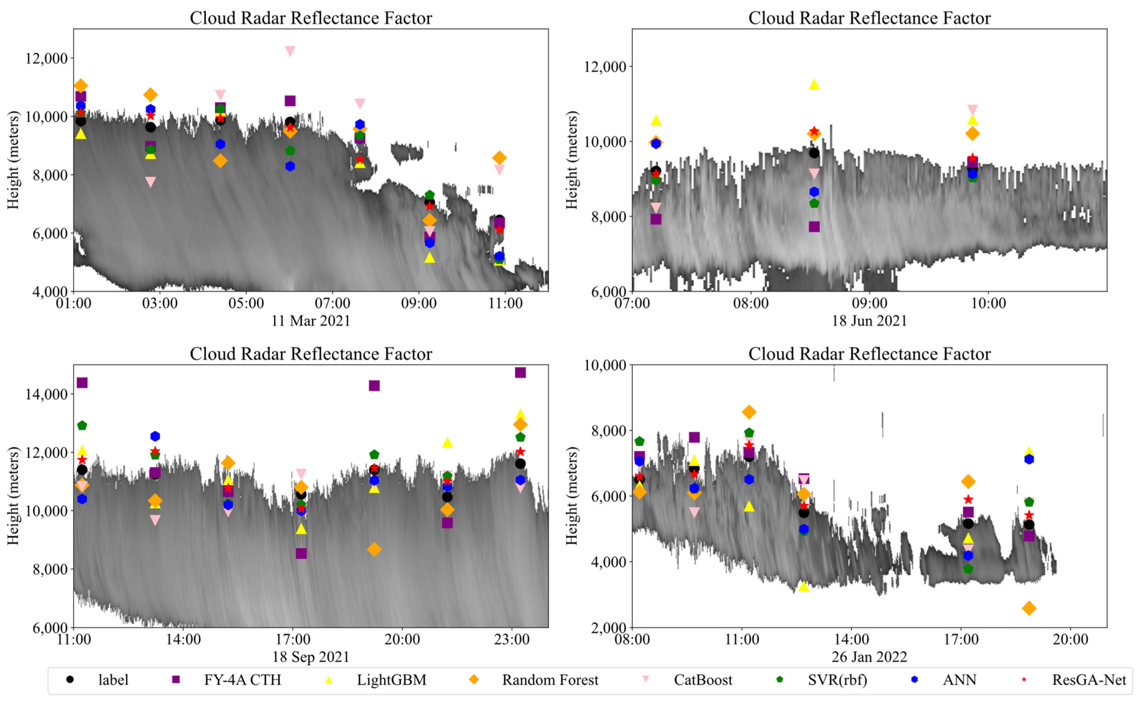
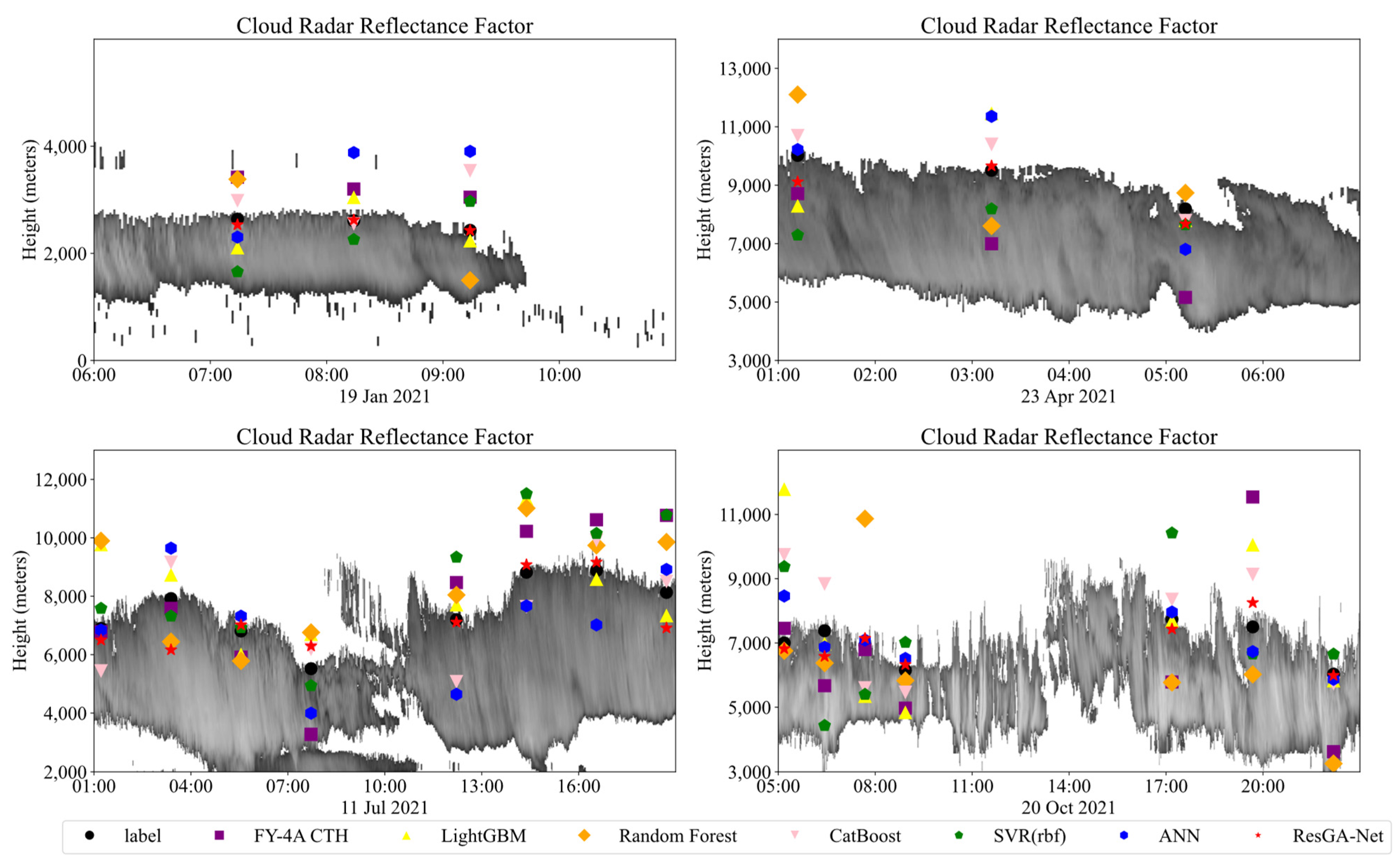
This paper selects representative cloud reflectance factor maps from the four seasons of the year to demonstrate the predictive performance of various algorithms, as shown in Figure 7. In these figures, the horizontal axis represents a 24 h timeline, while the vertical axis represents cloud height information in meters. The red pentagrams represent the results retrieved by the proposed ResGA-Net algorithm, while the black circles denote the ground truth observed by cloud radar. It can be observed that the predictions generated by the ResGA-Net algorithm proposed in this paper are generally closer to the underlying ground truth in most cases.

3.4. Ablation Study

To validate the effectiveness of our proposed ResGA-Net algorithm, we conducted an ablation study, the results of which are shown in

Table 2. Ablation study.

Algorithm/Evaluation Metric	RMSE (m)	MAE (m)	PCC	SRCC
ANN	1332.6	1072.4	0.814	0.806
ResGA-Net w/o GA	1281.3	1041.5	0.819	0.815
ResGA-Net w/o Residual-Enhanced NN	1179.1	966.9	0.830	0.824
ResGA-Net (ours)	1126.5	917.6	0.836	0.832

. It is worth noting that, when the genetic algorithm module and the residual-enhanced NN are removed from the model, ResGA-Net is reverted to the most basic artificial neural network (ANN). From Table 2, it can be observed that the introduction of the genetic algorithm (GA) module leads to the most significant improvement in model performance. Specifically, compared to the basic ANN, the RMSE decreases from 1332.6 m to 1179.1 m, a reduction of 11.51%, and the MAE decreases from 1072.4 m to 966.9 m, a reduction of 9.83%. Moreover, the PCC increases from 0.814 to 0.830, and the SRCC increases from 0.806 to 0.824. This demonstrates the effectiveness of using genetic algorithms for data selection. Secondly, the introduction of the residual-enhanced NN further improves the model. Compared to the basic ANN, the residual-enhanced NN increases the complexity and introduces residual-like structures to enhance the model stability, demonstrating better feature extraction capabilities. Compared to the basic ANN, the RMSE decreases from 1332.6 m to 1281.3 m, a reduction of 3.84%, and the MAE decreases from 1072.4 m to 1041.5 m, a reduction of 2.88%. Furthermore, the PCC increases from 0.814 to 0.819, and the SRCC increases from 0.806 to 0.815.

3.5. Regional Adaptability Validation

To validate the effectiveness of the satellite-ground combined method for retrieving CTH, this study employs the CTH prediction model from the Beijing Nanjiao Observatory to invert the CTH over the Beijing Fangshan Observatory located at 39°43′ N, 115°44′ E. Due to the considerable distance between the Nanjiao Observatory and the Fangshan Observatory, with a great circle distance of 63.15 km, data from the Fangshan Observatory can be used for algorithm regional adaptability verification.

The Beijing Nanjiao Observatory’s model is utilized to forecast the CTH over the Beijing Fangshan Observatory. The performance metrics of the inversion results are presented in

Table 3. Algorithm regional adaptability validation.

Algorithm/Evaluation Metric	RMSE (m)	MAE (m)	PCC	SRCC
FY-4A CTH	1953.8	1542.3	0.738	0.745
LightGBM	1732.4	1368.7	0.761	0.758
Random Forest	1609.8	1297.4	0.776	0.763
CatBoost	1565.5	1265.7	0.787	0.769
SVR_rbf	1506.3	1142.9	0.792	0.789
ANN	1412.0	1086.1	0.806	0.802
ResGA-Net (ours)	1182.2	949.3	0.829	0.825

. It is clear that, when the CTH retrieval model from the Beijing South Observatory is applied to CTH retrieval over the Beijing Fangshan Observatory, the RMSE and MAE metrics reach 1182.2 and 949.3, respectively. Compared to the CTH product data from FY-4A Fangshan Station, there is a reduction of 39.49% and 38.44%, respectively. Additionally, the PCC and SRCC metrics reach 0.829 and 0.825, showing an increase of 12.33% and 10.73%, respectively. This algorithm continues to demonstrate significant advantages and proves its good cross-regional performance.

The results of the model trained with Nanjiao Station data and other machine learning algorithm models on the data from Fangshan Station are shown in Figure 8. It is evident from the figure that the model trained with Nanjiao Station data (red pentagrams) generally performs the best on the Fangshan Station test data. The retrieved CTHs closely match those from ground-based cloud radar, with few significant deviations.

4. Conclusions

This paper proposes a new method for retrieving the cloud top height (CTH) by combining data from geostationary meteorological satellites and millimeter-wave cloud radar. The method utilizes a genetic algorithm module for data selection and employs a residual-enhanced neural network for modeling. By effectively utilizing the advantages of high-precision cloud radar observations and extensive coverage provided by geostationary meteorological satellites, this method significantly enhances the utilization of FY-4A and millimeter-wave cloud radar data, enabling the generation of high-precision CTH products.

The proposed ResGA-Net model was validated using data from Beijing spanning from January 2020 to January 2022. The results demonstrate that the ResGA-Net model outperforms FY-4A’s CTH product, with RMSE and MAE decreasing by 37.89% and 34.77%, while PCC and SRCC increase by 11.17% and 9.47%, respectively. Compared to other contrastive algorithms such as LightGBM, Random Forest, CatBoost, SVR_rbf, and ANN, this model also exhibits superiority in these four metrics. Furthermore, the model exhibits good cross-regional performance.

The current work mainly considers the multi-channel scan data from geostationary meteorological satellites as input features. In future work, consideration will be given to other factors that may affect CTH retrieval, such as observation location, solar radiation, and surface characteristics, to further improve the retrieval accuracy, rather than solely relying on satellite channel data. Additionally, comparisons will be made with other methods such as the stereoscopic observation method [30], which involves analyzing CTH data obtained from multiple perspectives or viewpoints to enhance accuracy and reliability.

References

1. Zhao, C.F.; Yang, Y.K. Progress and challenges of ground-based cloud remote sensing. Torrential Rain Disasters 2021, 40, 243–258. [Google Scholar]
2. Cao, Y.N.; Wei, H.L.; Dai, C.M.; Zhang, X.H. Retrieval of cloud optical thickness and cloud top height of convective clouds from AIRS infrared hyperspectral satellite data. Spectrosc. Spectr. Anal. 2015, 35, 1208–1213. [Google Scholar]
3. McFarquhar, G.M.; Bretherton, C.; Marchand, R.; Protat, A.; DeMott, P.J.; Alexander, S.P.; Roberts, G.C.; Twohy, C.H.; Toohey, D.; Siems, S.; et al. Observations of clouds, aerosols, precipitation, and surface radiation over the Southern Ocean: An overview of CAPRICORN, MARCUS, MICRE and SOCRATES. Bull. Am. Meteorol. Soc. 2020, 102, E894–E928. [Google Scholar] [CrossRef]
4. Liu, L.; Sun, X.J.; Gao, T.C. Retrieval of cloud parameters using ground-based infrared hyperspectral emissivity data (Part 1): Cloud phase discrimination. Spectrosc. Spectr. Anal. 2016, 36, 3885–3894. [Google Scholar]
5. Li, Z.; Niu, F.; Fan, J.; Liu, Y.; Rosenfeld, D.; Ding, Y. Long-term impacts of aerosols on the vertical development of clouds and precipitation. Nat. Geosci. 2011, 4, 888–894. [Google Scholar] [CrossRef]
6. Hong, Y.; Hsu, K.L.; Sorooshian, S.; Gao, X. Precipitation estimation from remotely sensed imagery using an artificial neural network cloud classification system. J. Appl. Meteorol. 2004, 43, 1834–1853. [Google Scholar] [CrossRef]
7. Gultepe, I.; Sharman, R.; Williams, P.D.; Zhou, B.; Ellrod, G.; Minnis, P.; Trier, S.; Griffin, S.; Yum, S.S.; Gharabaghi, B.; et al. A review of high impact weather for aviation meteorology. Pure Appl. Geophys. 2019, 176, 1869–1921. [Google Scholar] [CrossRef]
8. Zhu, X.L.; Qian, Y.Y.; Yan, W.; Li, G.; An, H. Application of cloud base height inversion algorithm based on multi-satellite observation results in China offshore waters. J. Meteorol. Sci. 2019, 39, 467–476. [Google Scholar]
9. Lu, Y.J.; Chen, G.Y.; Gong, K.J. Overview of researches on cloud sounding methods. Meteorol. Sci. Technol. 2012, 40, 689–697. [Google Scholar]
10. Duan, L.; Zhang, Y.; Guo, Y.P.; Zhao, Z. Research on Inversion of Convective Cloud Top Height Based on Infrared Brightness Temperature Method. Infrared 2022, 43, 33–40. [Google Scholar]
11. Gu, C.M.; Wang, Y.F.; Zhang, X.H.; Zhong, B.; Ma, X. Effects of cloud parameter on brightness temperature computation in microwave band. J. Appl. Meteorol. Sci. 2016, 27, 380–384. [Google Scholar]
12. Lee, J.; Shin, D.B.; Chung, C.Y.; Kim, J. A cloud top-height retrieval algorithm using simultaneous observations from the Himawari-8 and FY-2E satellites. Remote Sens. 2020, 12, 1953. [Google Scholar] [CrossRef]
13. Li, Q.; Sun, X.; Wang, X. Reliability evaluation of the joint observation of cloud top height by FY-4A and Himawari-8. Remote Sens. 2021, 13, 3851. [Google Scholar] [CrossRef]
14. Du, C.; Ren, H.; Qin, Q.; Meng, J.; Zhao, S. A practical split-window algorithm for estimating land surface temperature from Landsat 8 data. Remote Sens. 2015, 7, 647–665. [Google Scholar] [CrossRef]
15. Liang, Y.; Li, W.; Huang, Y. Retrieval of Semi-transparent Cloud Top Height Using Split Window Histograms Method. Acta Sci. Nat. Univ. Pekin. 2019, 55, 461–472. [Google Scholar]
16. Hamada, A.; Nishi, N. Development of a cloud-top height estimation method by geostationary satellite split-window measurements trained with CloudSat data. J. Appl. Meteorol. Climatol. 2010, 49, 2035–2049. [Google Scholar] [CrossRef]
17. Nishi, N.; Hamada, A.; Hirose, H. Improvement of cirrus cloud-top height estimation using geostationary satellite split-window measurements trained with CALIPSO data. SOLA 2017, 13, 240–245. [Google Scholar] [CrossRef]
18. Menzel, W.P.; Frey, R.A.; Zhang, H.; Wylie, D.P.; Moeller, C.C.; Holz, R.E.; Maddux, B.; Baum, B.A.; Strabala, K.I.; Gumley, I.E. MODIS global cloud-top pressure and amount estimation: Algorithm description and results. J. Appl. Meteorol. Climatol. 2008, 47, 1175–1198. [Google Scholar] [CrossRef]
19. Wang, F.; Zhao, Y. Cloud Top Height Retrieval Algorithm for Fengyun-4 Geostationary Meteorological Satellite. J. Sichuan Norm. Univ. (Nat. Sci. Ed.) 2021, 44, 412–418. [Google Scholar]
20. Yu, Z.F.; Wang, Y.; Ma, S.; Ai, W.H. An Ensemble Learning-Based Method for FY-4A Cloud Base Height Retrieval. Acta Opt. Sin. 2023, 43, 49–62. [Google Scholar]
21. Dong, Y.; Sun, X.; Li, Q. A Method for Retrieving Cloud-Top Height Based on a Machine Learning Model Using the Himawari-8 Combined with Near Infrared Data. Remote Sens. 2022, 14, 6367. [Google Scholar] [CrossRef]
22. Rysman, J.F.; Claud, C.; Dafis, S. A machine learning algorithm for retrieving cloud top height with passive microwave radiometry. IEEE Geosci. Remote Sens. Lett. 2021, 19, 4500605. [Google Scholar] [CrossRef]
23. Katoch, S.; Chauhan, S.S.; Kumar, V. A review on genetic algorithm: Past, present, and future. Multimed. Tools Appl. 2021, 80, 8091–8126. [Google Scholar] [CrossRef]
24. Aggarwal, C.C.; Yu, P.S. An effective and efficient algorithm for high-dimensional outlier detection. VLDB J. 2005, 14, 211–221. [Google Scholar] [CrossRef]
25. Zhang, T.H.; Bao, Y.S.; Qian, Y.Z.; Lin, L.B.; Liu, X.L.; Li, L.; Hou, Y.; Lei, H.Y.; Li, G.W.; Ma, J.; et al. Atmospheric temperature and humidity profile retrievals based on BP neural network and genetic algorithm. J. Trop. Meteorol. 2020, 36, 97–107. [Google Scholar]
26. Li, T.; Li, N.P.; Qian, Q.; Xu, W.; Ren, Y.; Xia, J.Y. Inversion of temperature and humidity profile of microwave radiometer based on bp network. Intell. Autom. Soft Comput. 2021, 29, 741–755. [Google Scholar] [CrossRef]
27. Li, T.; Qiao, C.; Wang, L.; Chen, J.; Ren, Y. An algorithm for precipitation correction in flood season based on dendritic neural network. Front. Plant Sci. 2022, 13, 862558. [Google Scholar] [CrossRef]
28. He, K.; Zhang, X.; Ren, S.; Sun, J. Deep Residual Learning for Image Recognition. In Proceedings of the 2016 IEEE Conference on Computer Vision and Pattern Recognition (CVPR), Las Vegas, NV, USA, 27–30 June 2016. [Google Scholar]
29. Ioffe, S.; Szegedy, C. Batch normalization: Accelerating deep network training by reducing internal covariate shift. In Proceedings of the International Conference on Machine Learning 2015, Lille, France, 6–11 July 2015; pp. 448–456. [Google Scholar]
30. Huang, Y.X.; Ma, S.; Bai, H. Error analysis of cloud top height detection using stereoscopic observation method. J. Infrared Millim. Waves 2012, 31, 314–318. [Google Scholar] [CrossRef]
Figure 1. Overall structure of ResGA-Net. It mainly consists of two modules: (i) a genetic algorithm module used to enhance the quality of the training dataset and (ii) a residual-enhanced NN that is used to train neural networks from the selected training data and evaluate them using the testing dataset.
Atmosphere 15 00643 g001
Figure 2. Chromosome encoding schematic. This is an example of chromosome gene encoding corresponding to the dataset samples. Each gene in the chromosome represents whether a sample is retained, encoded as 1 for retention and 0 for discard (denoted by a red “X” in the figure). The dataset formed by the retained samples is used for the subsequent residual-enhanced NN modeling.
Atmosphere 15 00643 g002
Figure 3. Schematic diagrams of randomly divided data (a) and compute temporary fitness (b). (a) The random division of the dataset corresponding to the chromosomes into three groups for the fitness calculation in (b). (b) The establishment of a BP neural network using the data divided in (a) to calculate the fitness of the chromosomes.
Atmosphere 15 00643 g003
Figure 4. Overall structure of the residual-enhanced NN. The entire network consists of six layers, including input and output layers, as well as four hidden layers. In the diagram, yellow shapes represent the batch normalization (BN) layer, blue shapes represent the fully connected layer, and red shapes represent the sigmoid activation layer. The green arrow indicates the data flow direction.
Atmosphere 15 00643 g004
Figure 5. Scatter plots of various algorithms with cloud radar data. The vertical axis represents the CTH values obtained from cloud radar, while the horizontal axis represents the predicted results of various algorithms. The closer the points are to the central dividing line (representing y = x), the closer the predicted results are to the radar data. The comparison methods are (a) FY-4A CTH, (b) LightGBM, (c) Random Forest, (d) CatBoost, (e) SVR_rbf, (f) ANN, and (g) ResGA-Net (ours).
Atmosphere 15 00643 g005
Figure 6. The histogram of errors between the predicted results of various algorithms and the cloud radar data, with a bin width of 600 m. The vertical axis of each subplot represents the number of samples, while the horizontal axis represents the errors between the algorithm’s predicted results and the radar data. The comparison methods are (a) FY-4A CTH, (b) LightGBM, (c) Random Forest, (d) CatBoost, (e) SVR_rbf, (f) ANN, and (g) ResGA-Net (ours).
Atmosphere 15 00643 g006
Figure 7. The example of a cloud radar reflectivity factor map at Beijing Nanjiao Station selected from the four seasons of the year. To enhance clarity, a portion of the reflectivity factor map containing clouds was selected, and areas without clouds at certain time intervals and height levels were discarded. In the figure, the black circles represent the cloud top heights measured by the cloud radar. The purple squares, yellow triangles, orange diamonds, pink inverted triangles, green pentagons, blue hexagons, and red pentagrams, respectively, represent the CTH product data from FY-4A and the predicted results from LightGBM, Random Forest, CatBoost, SVR (rbf), ANN, and ResGA-Net.
Atmosphere 15 00643 g007
Figure 8. The example of a cloud radar reflectivity factor map at Beijing Fangshan Station selected from the four seasons of the year. To validate the model’s cross-regional capability, models trained with data from the Nanjiao Station were utilized to test the Fangshan Station. For clarity, the figure still cropped out the cloud-free areas of the reflectivity factor map along the time axis and height layers. The legend is consistent with that in Figure 7.
Atmosphere 15 00643 g008