Article

Numerical Simulation of the Plant Shelterbelt Configuration Based on Porous Media Model

1
Key Laboratory of Mechanics on Disaster and Environment in Western China, Lanzhou University, The Ministry of Education of China, Lanzhou 730000, China
2
College of Civil Engineering and Mechanics, Lanzhou University, Lanzhou 730000, China
3
Gansu Minqin National Station for Desert Steppe Ecosystem Studies, Gansu Desert Control Research Institute, Wuwei 733000, China
4
Zhengzhou Design Institute, China Railway Engineering Design and Consulting Group Co., Ltd., Zhengzhou 450001, China
*
Author to whom correspondence should be addressed.
Atmosphere 2024, 15(5), 602; https://doi.org/10.3390/atmos15050602
Submission received: 1 April 2024 / Revised: 30 April 2024 / Accepted: 11 May 2024 / Published: 14 May 2024
(This article belongs to the Section Biosphere/Hydrosphere/Land–Atmosphere Interactions)

Abstract

:
Low-coverage line-belt-pattern protective forests offer significant advantages in terms of wind and sand control measures. It is important to study the windbreak effectiveness of sand-fixing forests with different spacing for the construction and optimization of plant shelterbelt configurations. The effect of plant spacing on the flow field around a row of trees was investigated using the k-ε turbulence model coupled with the porous media model. In order to accurately simplify the complex and stochastic plant constitutive features, we simplify the plant canopy to a circular platform geometry, which introduces a porous media model, and the plant trunk is simulated as a solid cylinder. The simulation results show that windbreaks only affect wind profiles up to 1.25-times the height of the tree; on the leeward side of the canopy, large-spaced shelterbelts provide greater protection in the near-wake zone, while small-spaced shelterbelts are more effective at reducing velocity in the re-equilibration zone. The flow field recovery properties of the trunk and canopy indicate that the canopy wake zone is longer. In this study, we also quantitatively analyze the relationship between average wind protection effectiveness as a function of plant spacing and streamwise distance from the leeward side of the canopy, and the given parameterized scheme shows a power exponential relationship between wind protection effectiveness and plant spacing and a logarithmic relationship with streamwise distance. This scheme can provide a predictive assessment of the effects during the implementation of the plant shelterbelt.

1. Introduction

In arid and semi-arid areas, plant-based sand control measures are renewable and can also increase the water-holding capacity in the desert, which is considered to be a fundamental, economic and effective measure [1]. However, due to the constraints of water resources, the density of afforestation of sand fixation forests should not be too high. Consequently, it is imperative to minimize wind velocities within the reserve by employing the minimum number of trees. The selection of tree species and configuration of the shelterbelt structure have a significant impact on wind protection [2].
The line-belt pattern is a composite vegetation pattern that consists of a combination of forest belts and natural vegetation restoration belts, where “line” refers to one or more rows of trees in a plantation and “belt” refers to the space between the forest belts, also known as the vegetation restoration belt [3]. There are a number of factors that affect the effectiveness of protection in line-belt wind and sandbreak forests [4]. For single plants, the height [5], porosity [6], shape [7], branch and leaf flexibility [8] of their canopy all have an impact on the wind field. Dong et al. found that the higher the porosity, the less resistance the airflow encounters as it passes through the vegetation, and the wind speed is weakened less. When porosity is very low, the airflow encounters greater resistance and is lifted upwind of the vegetation, creating a strong vortex in the vicinity of the vegetation, thus shortening the protection distance [9]. Therefore, there exists an optimal porosity to maximize wind protection effectiveness. Due to the huge number and complexity of plant branches and leaves, in numerical simulation, researchers usually consider the canopy as a porous region and make various simplifications of its shape. Svensson et al. and Gash simplified the 3D canopy to a 2D rectangle to study the flow field distribution characteristics [10,11], but the two-dimensional flow field ignores the vertical and lateral flow of the airflow, which makes the simulation result deviate a little from the actual one.
For a community structure formed by the combination of multiple plants, the line-belt pattern has obvious advantages in the comprehensive consideration of wind-preventing and sand-fixing effects, water use efficiency, and later maintenance and management factors, and the factors affecting the wind protection effectiveness of plant communities in the line-belt pattern are row spacing, belt spacing, plant spacing, belt width, etc. The study found that the higher the number of rows in the forest belt, the more effective it is in wind protection [12,13]. Cheng et al. investigated the variation in the wind protection effect of forest belts with one to five rows and found that the number of rows in the shelterbelts increases, and its windbreak effect increases gradually but in a nonlinear manner [8]. For example, Rosefeld found that the protection distance of a multi-row forest belt increased by only 10% compared to a single-row forest belt [14]. However, for wind and sand control, the width of the forest belt does not follow the pattern of the greater the better, and there is a critical value. Li et al. studied the effective protection area of shelterbelts with different numbers of rows and found that, between two rows and six rows, the higher the number of rows, the higher the shelter efficiency of the shelterbelts, but the shelter efficiency of the eight-row shelterbelts was not as good as that of the six-row ones, which indicated that the width of the forest belt was not positively correlated with the shelter efficiency after a certain point [2]. Comprehensively considering the wind protection effect and water use efficiency and other factors, for plants with well-developed root systems, it is ideal to arrange them in single-row or double-row arrangements to prevent wind and fix the sand [3]. The above work focuses on the research and analysis of the relatively complex line-belt pattern structure, but, so far, our analysis of spacing of plants in line-belt windbreaks on the flow structure and the mechanism of its effect on wind and sand conservation is still insufficient, which limits the analysis of sand and windbreaks and the optimization of arrangement patterns under the multi-line-belt pattern model. Therefore, this study takes the simplest one-row forest belt as the basis, simplifies plant canopies into porous media, studies the effect of plant spacing on the wind field, and proposes the relationship between the spacing of the one-row shelterbelts and windbreak effectiveness, so as to provide a reference for the optimization of the configuration of artificial protection forests in arid and semi-arid areas.

2. Materials and Methods

2.1. Modeling of Porous Media in Plant Canopies

The canopy of the tree is very different from the trunk, and it forms a windbreak that plays a significant role in reducing wind speeds, consolidating sandy soils, and improving the climate [3]. However, in arid and semi-arid areas, the climate and soil conditions are very harsh so the tree species for afforestation should meet the characteristics of drought and barrenness tolerance. In this regard, Yang et al. gave more than ten sand-fixing tree species suitable for low-coverage line-belt silviculture, such as Ulmus pumila, Salix matsudana, and Populus euphratica, with different canopy patterns [3].
In this study, we simulate the trees with a spherical canopy shape and describe the complex structure inside of the canopy as the porous media. There are many examples of using porous media to simulate the plant canopy [15,16,17,18]. Compared to using numerical methods to directly simulate the interaction of fluids and solids in the canopy, the latter requires high-resolution meshes to characterize small-scale structures, and the computation takes a tremendous amount of time and memory. But the additional source term method is used to model the action of porous media by adding a source term to the momentum equation, which is computationally fast and feasible [19]. Endalew et al. attempted to establish a very complex physical model for calculation according to the real situation of plants and, compared with the standard homogeneous porous model of the canopy, found that the former is not only computationally inefficient but, also, the results of the two calculations are basically the same [20].
Figure 1 shows a velocity vector comparison between the porous media canopy and the impenetrable solid canopy on the leeward side. It can be seen that the deceleration zone on the leeward side of the porous media canopy is obviously longer than that on the leeward side of the impenetrable solid canopy, and there exists a certain size of the reflux zone on the leeward side of the impenetrable solid canopy, which is almost invisible on the leeward side of the porous media. This is due to the fact that the flow characteristics behind the canopy with a void nature are significantly different from those in the leeward zone of the impenetrable solid; this difference has been observed in wind tunnel experiments and in the field [21]. This is shown by the longer reflux zone and less turbulence [22] in the leeward region of the void structure, meaning that the wind velocity has a longer distance to return to the incoming velocity after being weakened [23], so using the porous media model more accurately describes the problem described in this study.
The source term of the momentum equation consists of the viscous loss term and the inertial loss term with the following expression:
S i = j = 1 3 D i j μ u i + j = 1 3 C i j 1 2 ρ u u i
where Cij and Dij are resistance coefficient matrices.
In the model in this study, the Reynolds number of the airflow is relatively large, and the viscous loss term is not in the same order of magnitude as the inertial loss term, so the viscous loss term can be neglected, and Si is simplified as:
S i = 1 2 C i ρ u u i
where Ci is the inertial resistance factor.

2.2. Governing Equations

The continuity equation and the momentum equation with an added source term are written, respectively:
u i x i = 0
ρ u i u j x j = p x i + x j μ u i x j + u j x i ρ x j u i u j ¯ + S i
where ui is the i component of the average air velocity, ui′ is pulsation value of the average speed ui, xi and xj are Cartesian coordinates, μ is the dynamic viscosity, ρ is the density, p is the pressure, and Si is the momentum source term, which exists only in the canopy.
The Reynolds stresses are modeled as:
u i u j ¯ = μ t ρ u i ¯ x j + u j ¯ x i 2 3 k δ i j
where μt is the turbulent viscosity and δij the Kronecker delta; k is turbulent kinetic energy.
In this study, we use ANSYS Fluent software (https://www.ansys.com/products/fluids/ansys-fluent) to solve the governing equations, and the standard k-ε model, which is the most widely used, is adopted. Its turbulent kinetic energy and dissipation rate equations are, respectively:
ρ k t + ρ k u i x i = x j μ + μ t σ k k x j + μ t u i x j + u j x i u i x j ρ ε
ρ ε t + ρ ε u i x i = x j μ + μ t σ ε ε x j + μ t C 1 ε ε k u i x j + u j x i u i x j C 2 ε ρ ε 2 k
From the recommended values given by Launder et al. combined with later experimental verification, the empirical constants (C1ε, C2ε) and Prandtl numbers (σε, σk) corresponding to turbulent kinetic energy dissipation rate ε and turbulent kinetic energy k take the values of C1ε = 1.44, C2ε = 1.92, σε = 1.3, σk = 1 [24].

2.3. Model Validation

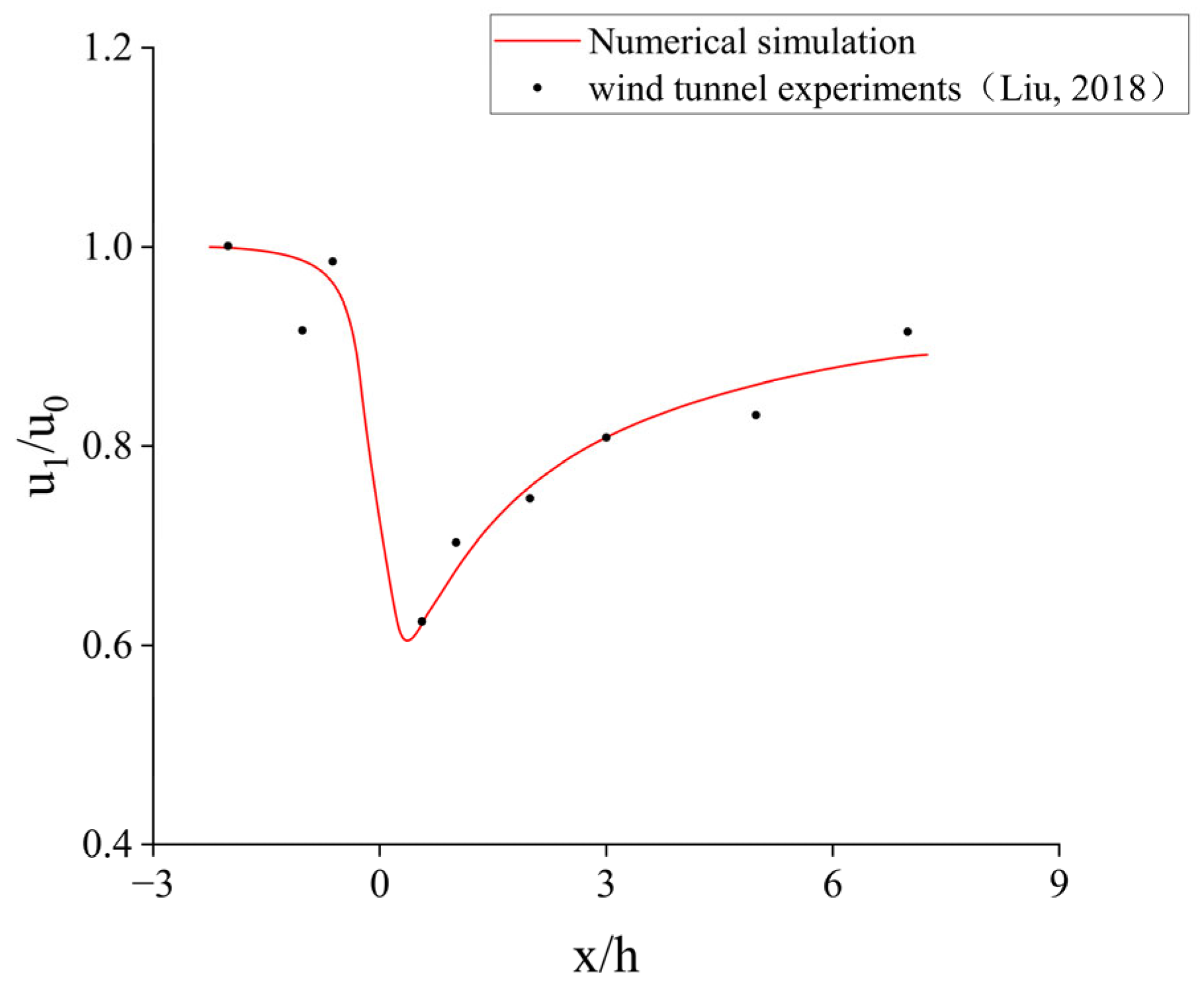
The complexity of the tree canopy and the uncertainty of the branch and leaf distribution make it difficult to determine the value of the inertial resistance factor. In order to determine the value of the canopy inertial resistance factor (Ci), we first simplify the canopy as a cylinder, with a diameter of 0.1 m and a height of 0.2 m. By comparing with the results of wind tunnel experiments [25], it is found that Ci taking 17.5 m−1 is in better agreement with the measured results (Figure 2).

2.4. Computational Modeling and Boundary Conditions

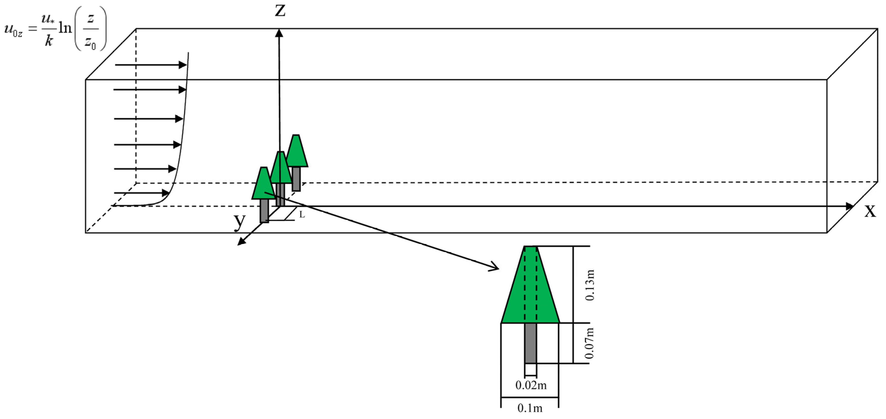
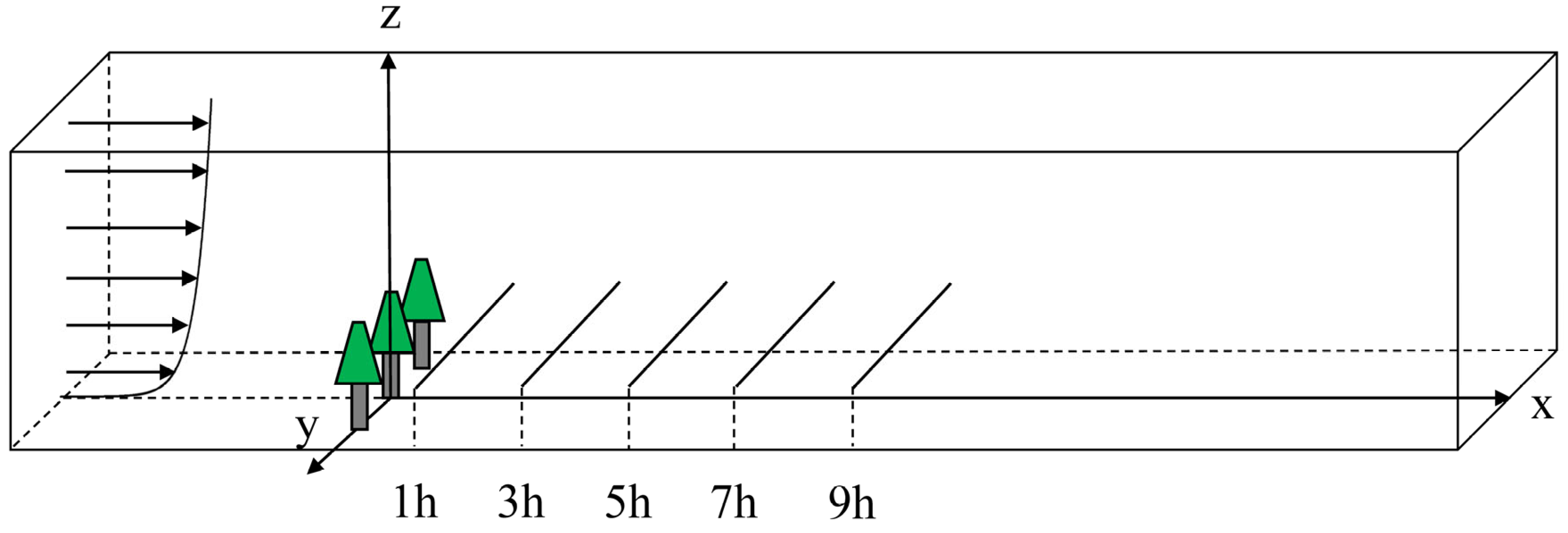
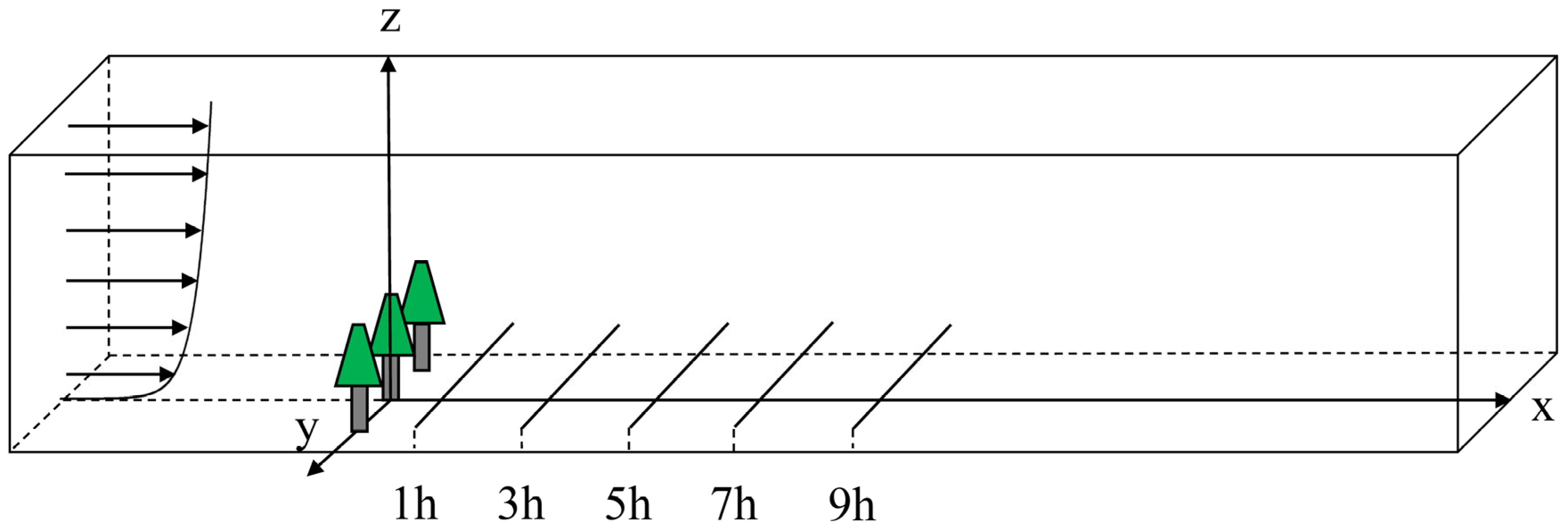
As shown in Figure 3, in order to simulate a tree with a spherical canopy, in this study, the plant trunk is approximated as a solid cylinder, with a diameter of 0.02 m and a height of 0.07 m, and the plant canopy is approximated as a circular platform, with a height of 0.13 m, a top diameter of 0.02 m, and a bottom diameter of d = 0.1 m. Combining the above studies, the canopy was simulated as porous medium, inertial resistance factor Ci was taken as 17.5 m−1, and the height of the whole plant model h = 0.2 m. The computational domain was 5.1 m in length (5 h before and 20 h after the plant model), 1 m in width (5 h), and 1 m in height (5 h), which corresponds to the minimum computational domain height recommended by Blocken [26].
Three plants were set up in the center of the wind field, which was modeled as a row of trees by the symmetry boundary. The spacing of the “one line and one band pattern” of windbreaks was taken as L = 0.78 h (1.56 d), 1 h (2 d), 1.25 h (2.5 d), and 1.5 h (3 d), respectively, and the length and height of the computational domain were constant, with its width varying with plant spacing. However, no matter how the width is changed, the origin of the coordinate system is always taken at the bottom of the plants in the center of the forest belt, and the coordinate axes in three directions are shown in Figure 2.
The left boundary of the computational domain is set as the inlet, and the inlet wind velocity is given in the form of a logarithmic profile:
u 0 z = u * κ ln z z 0
where u* is the frictional velocity, k is the von Karman constant, and z0 is the aerodynamic roughness.
The right boundary is set as outflow boundary, the top and lateral boundaries are set as symmetry boundaries, the bottom and trunk surfaces are set as stationary walls with no slip, and the canopy surface is set as internal boundary.
The structured grid is delineated using ICEM, with the maximum grid size set at 0.02 m and encrypted near the canopy and at ground level, using a total of about 2 million grids. The control equations are solved using ANSYS fluent, and the SIMPLE algorithm is chosen to decouple velocity form pressure. The discretization method used is the second-order upwind scheme. The steady-state simulation calculations are considered converged when the residuals of each term fall below 10−6, which typically requires several thousand iterations.

3. Results and Discussion

3.1. Flow Field Analysis of a Single Plant

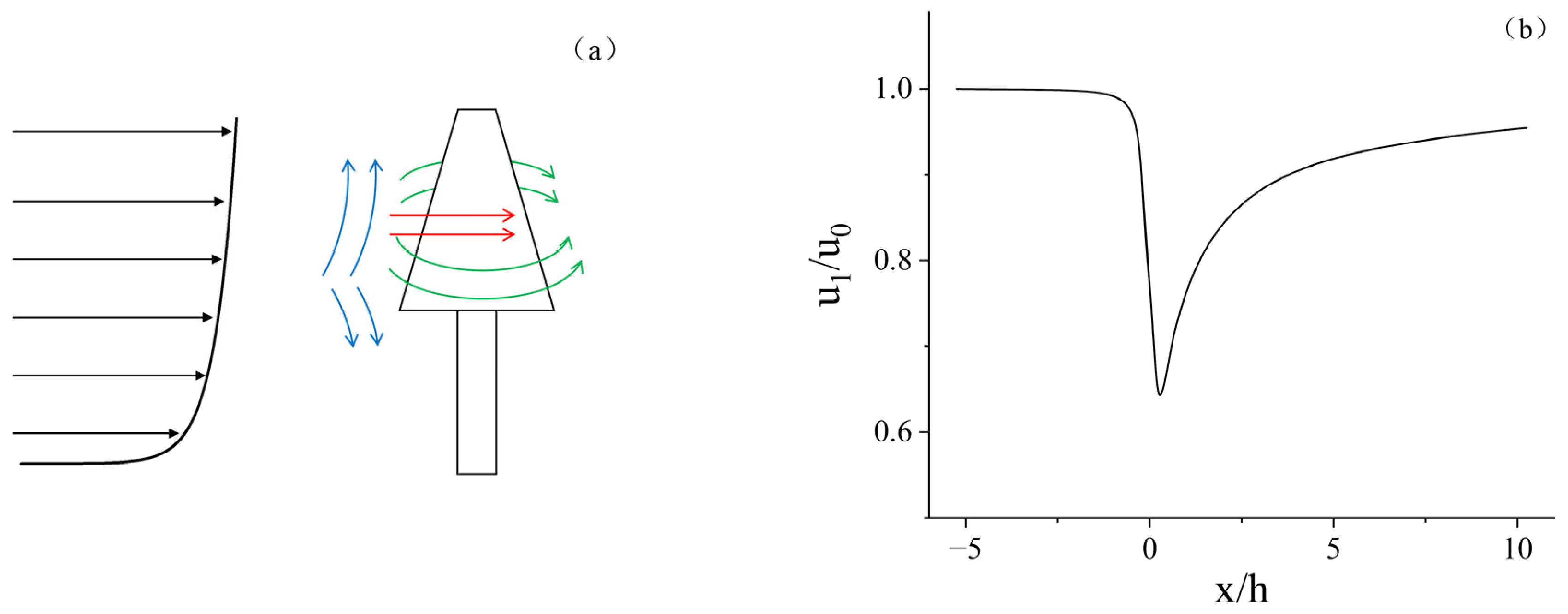
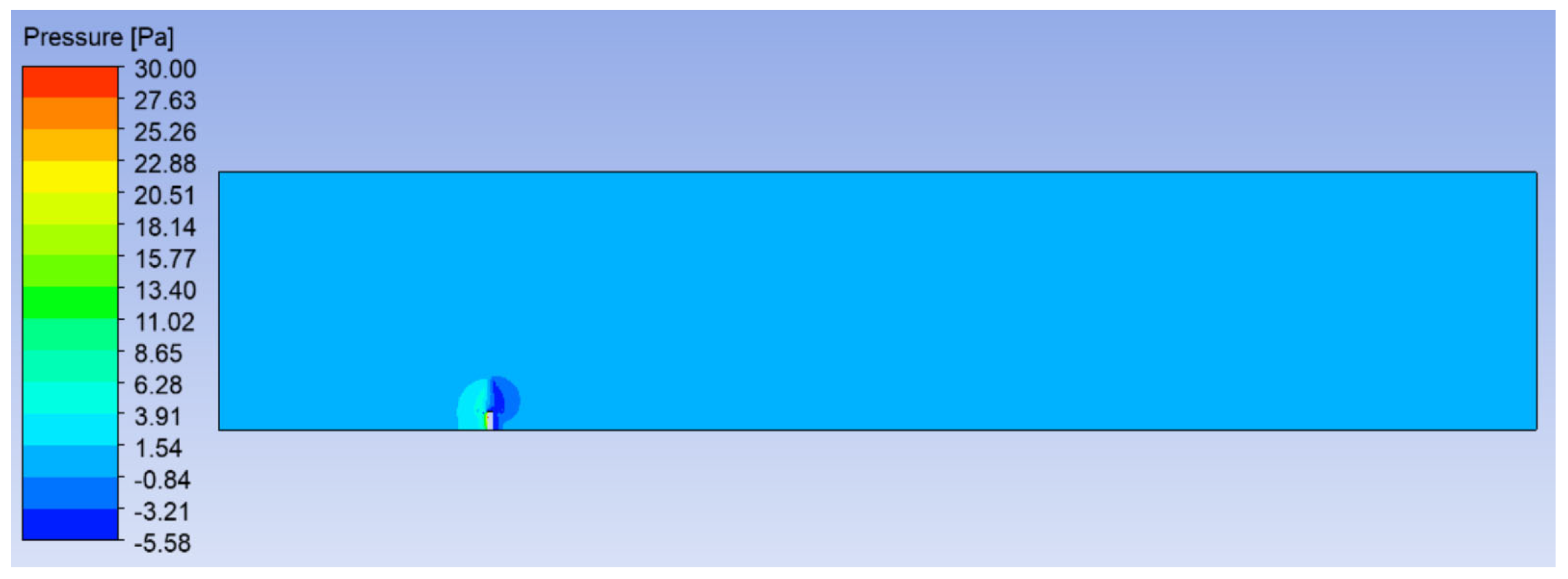
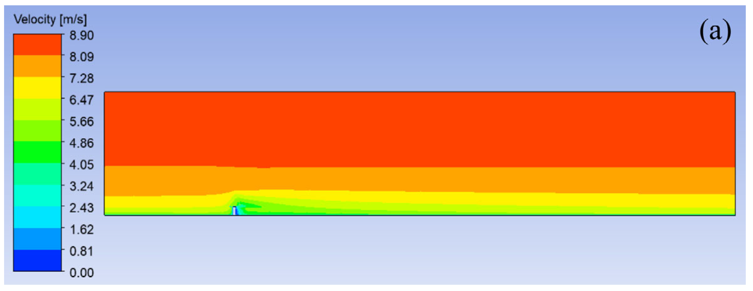
Figure 4a represents the airflow flow on the windward side of a single plant canopy, which is componentized in the X, Y, and Z directions due to the obstruction of the porous media. Firstly, the effect of individual plants on the x-direction velocity is analyzed. As can be seen in Figure 4b, the velocity on the leeward side of the canopy is reduced, which is the result of the effect of canopy resistance. After that, the velocity gradually recovered, and the wind velocity recovered to about 90% of the incoming wind velocity at 4 h on the leeward side, which is consistent with Liu’s results [25]. The pressure field in the symmetry plane is shown in Figure 5, and it can be found that the large pressure is at the windward leading edge of the canopy because the airflow is obstructed by the canopy, and part of the airflow will flow in the opposite direction, so the airflow stagnation area is formed on the windward side of the canopy, which produces a large positive pressure area. The obstruction of airflow by the canopy also caused the blockage effect, giving rise to cross flow perpendicular to the direction of incoming flow.
In general, cross flow will exist both laterally and vertically, but in reality, the geometry of the obstacle has a significant impact on the flow of the airflow [27]. The shape of the canopy modeled in this study is a circular platform that is narrow at the top and wide at the bottom, and this irregular shape can lead to uneven pressure [14], so the upward flow was observed to be much larger than the downward flow in front of the plant (x = −0.5 h), and its velocity also increased with height, reaching a maximum at the top of the canopy, as shown in Figure 4d, which is also in accordance with Moshe Rosenfeld’s findings [14]. This part of the upward airflow merges with the original airflow at the top of the canopy, creating a high-wind-speed zone above the plant [28], as shown in Figure 6a.
The lateral cross flow is faster compared to the vertical cross flow, which is also due to the shape of the canopy. As can be seen in Figure 4c and Figure 6b, the lateral cross flow on both sides of the canopy gradually increases within the canopy, reaches a maximum velocity at the edge of the canopy, and gradually decreases in velocity as it flows out of the canopy, with the lateral wind speed decreasing to less than 0.01 of the incoming wind speed beyond y > 0.75 h. At this point, we consider the effect of the plant on the wind field here to be negligible, so the furthest plant spacing in this study is chosen to be 1.5 h (3 d).

3.2. Sensitivity Analysis of the Plant Spacing Variation

3.2.1. Vertical Velocity Profiles

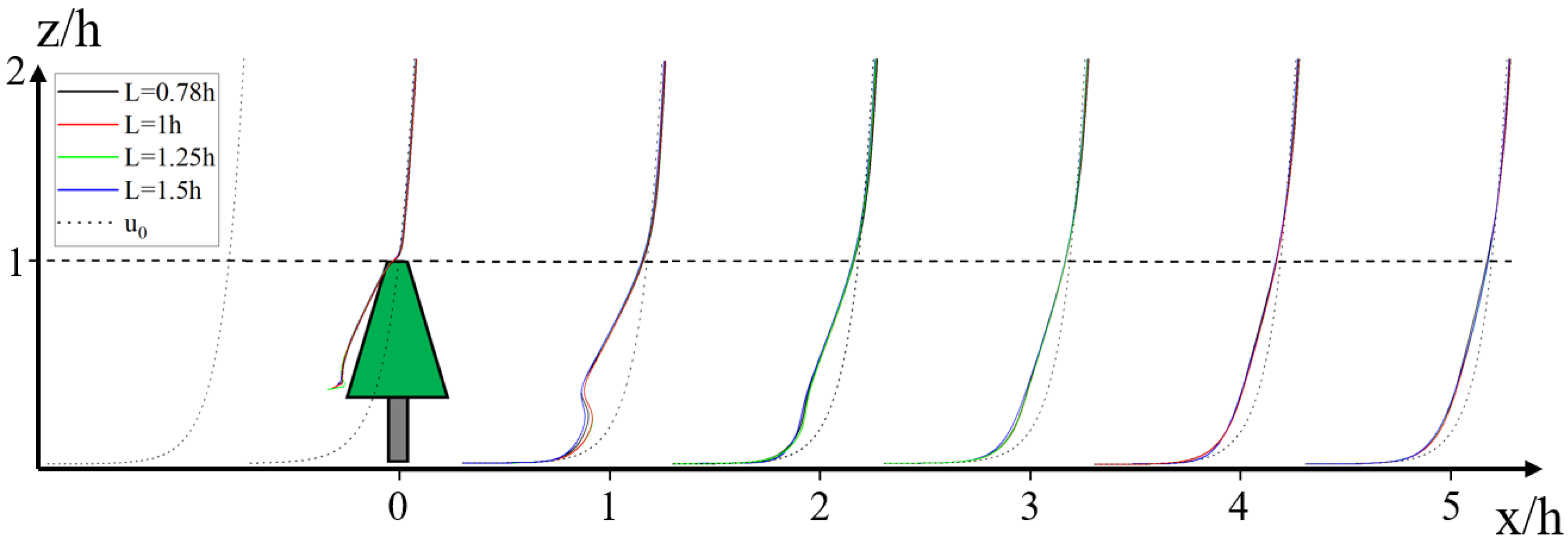
In order to analyze the effect of plant spacing on the wind field at different heights and distances on the leeward side of the forest belt, the variation in vertical velocity profiles along the streamwise direction in the center of the forest belt with different plant spacings was plotted at y = 0, as shown in Figure 7. It can be observed that the wind profiles are significantly distorted on the leeward side when the airflow is obstructed by plants, followed by a gradual recovery of the velocity; after 3 h on the leeward side, flow perturbations by the windbreak are smoothened until the approaching wind is reestablished [29]. The longer trails of horizontal wind speed shown in Figure 7 compared to the actual situation may be attributed to the relatively low canopy resistance coefficient, which prevents the wind speed from recovering quickly to the incoming wind speed. Alternatively, it could be due to the limitations of the model based on the Boussinesq hypothesis.
Above the plants, due to canopy obstruction, similar to the flow field of a single tree, part of the airflow also flows upward, creating an acceleration zone above the forest belt (Figure 7). The acceleration zone wind speed increases with decreasing plant spacing, and this acceleration zone gradually moves upward with streaming distance. Before the log-law boundary layer flow is reestablished, this acceleration zone can move up to 1.25 h.
Raupach summarizes the profiles of single-point turbulence statistics measured in some separate experiments [30]. We compared the vertical velocity profiles above the plants with them and found general agreement (Figure 8). The reason for this difference is that the vertical velocity profiles summarized by Raupach are mainly for forests, which have larger porosity. But we studied a row of trees, where the porosity is smaller and the drag coefficient is also smaller, so the obstruction effect on the airflow is not so strong and will not make the airflow flow upward too much, so the wind speed we calculated is lower above the height at 1 h and higher below the height at 1 h.
In contrast, below 1.25 h of height, the presence of the forest belt significantly reduced the wind speeds. Upon analyzing Figure 7, it is evident that while both the plant canopy and trunk reduce wind speed, the degree and mechanism of velocity reduction differ between the upper and lower layers. The difference in degree between the two is particularly evident in the significant reduction in velocity on the leeward side of the canopy of porous media, and the gradual increase in the efficiency of velocity reduction from the top of the canopy to the bottom of the canopy, with the efficiency of wind protection reaching its maximum at the bottom of the canopy. However, the trunk is a relatively weak speed barrier. Therefore, the understory leeward of the tree has a higher velocity. On the leeward side of the forest belt, there is a constant exchange of momentum between the high-velocity underlayer and the low-velocity upper region, so a log-law boundary layer flow is reestablished [25].
In order to analyze the difference between the effects to the wake region of the canopy and the trunk, we will examine each of them individually.

3.2.2. Influence of Canopy on the Flow Field

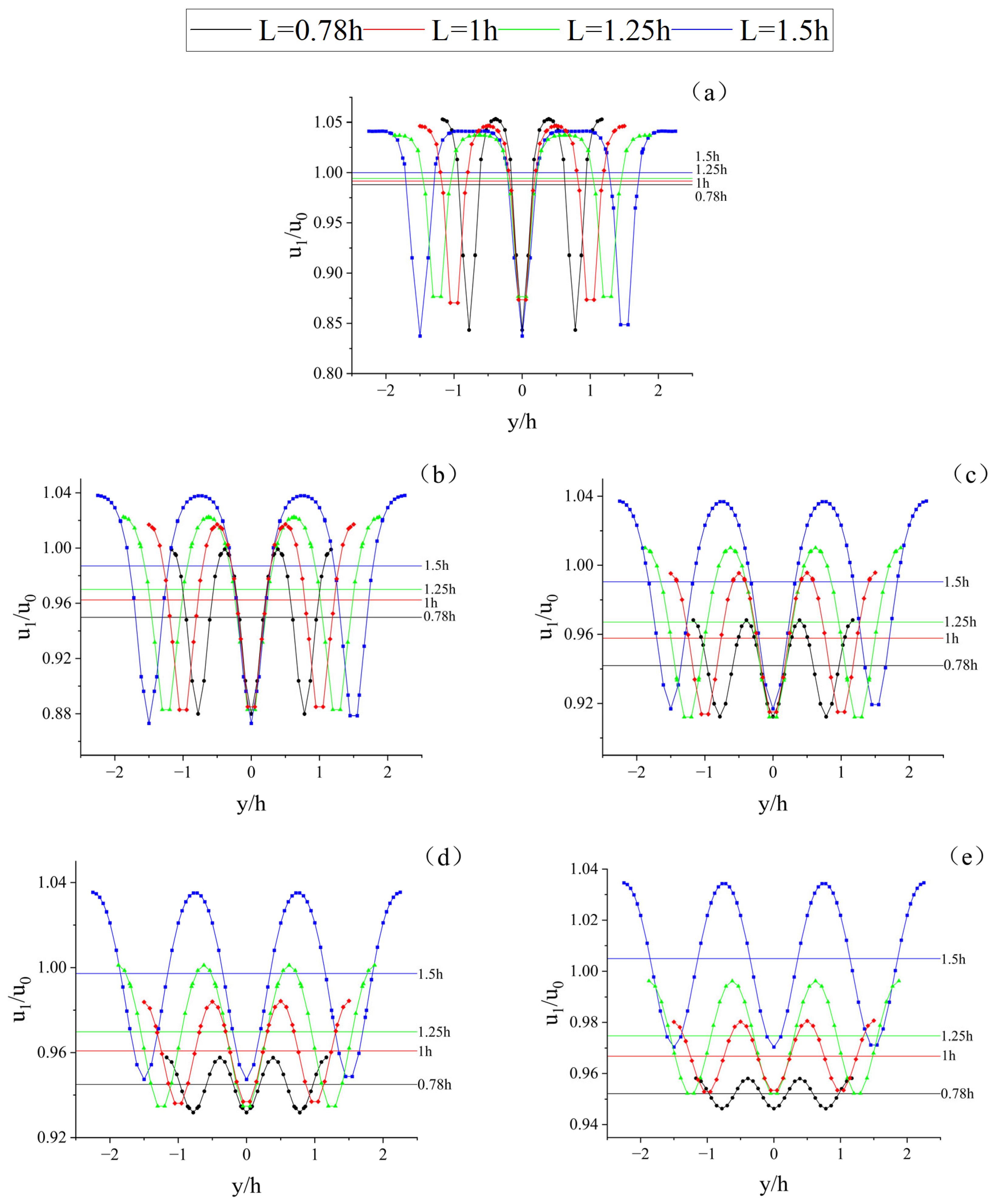
In order to analyze the obstruction of the wind field by the canopy, 1/2 of the height of the tree was taken for the study, as shown in Figure 9. Figure 10 shows the variation in velocity along the characteristic line for forest belts with different spacing.
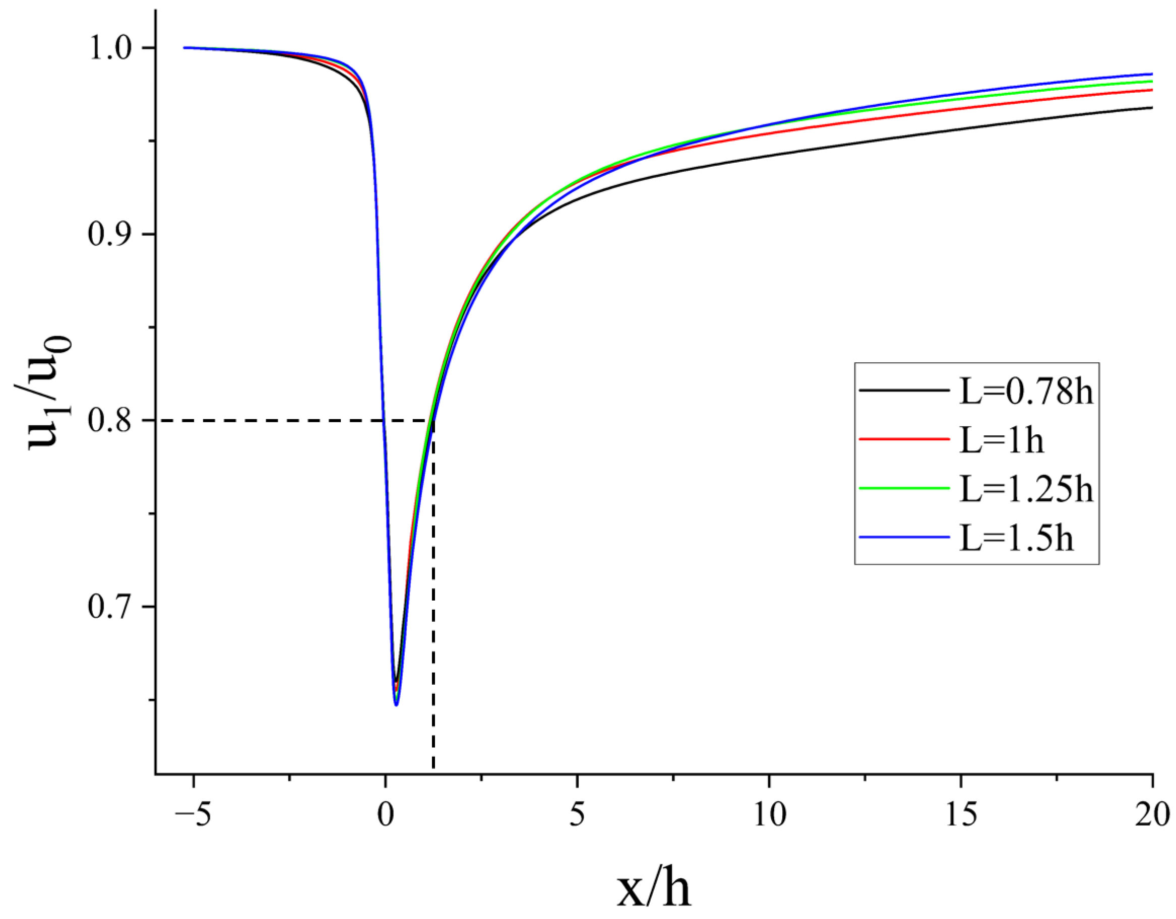
As can be seen in Figure 10, similar to a single tree, the airflows are all slowed down by the obstruction of the porous media and flow out in the form of the bleeding flow. On the leeward side of the plant, the bleeding flow from the canopy exchanges momentum with the displaced flow passing around the plant, and the velocity gradually recovers [27]. The recovery curve shows an exponential pattern of “first fast, then slow”, which has been found in many studies [5,8].
Using the distance d20 at which the wind speed on the leeward side of the forest belt returns to 80% of the incoming wind speed to define the protection distance of the shelterbelt [21,31], it can be found that the protection distances of the four windbreaks are between 1 h and 2 h. This result is similar to Cheng’s study on single rows of trees [8].
Analyzing the velocity on the characteristic line shown in Figure 9, it was found that the minimum value of velocity (umin) appeared at the same location in the wind field with different spacing, and its values were in the following order from smallest to largest: u1.5h, u1.25h, u1h and u0.78h. However, at 20 h on the leeward side of the forest belt, the velocities on the median axis of the forest belt at different spacing were, in descending order: u0.78h, u1h, u1.25h and u1.5h. This suggests that large-spaced forest belts provide better protection in the near-wake region, while small-spaced forest belts have a more pronounced weakening effect on the wind field in the re-equilibration zone.
We compared the extent to which different spacings at different distances from the leeward side of a forest belt weaken the velocity on the median axis: At 0–0.5 h, the larger the plant spacing, the greater the wind protection efficiency; at 8.5–20 h, the smaller the plant spacing, the greater the wind protection efficiency; however, between 0.5 and 8.5 h, the relationship between wind protection efficiency and plant spacing is difficult to determine. But it is worth mentioning that at 0.5–3 h, the forest belt with a spacing of 1.5 h was the most effective against velocity, while at 3–8.5 h, the forest belt with a spacing of 0.78 h weakened velocity the most.
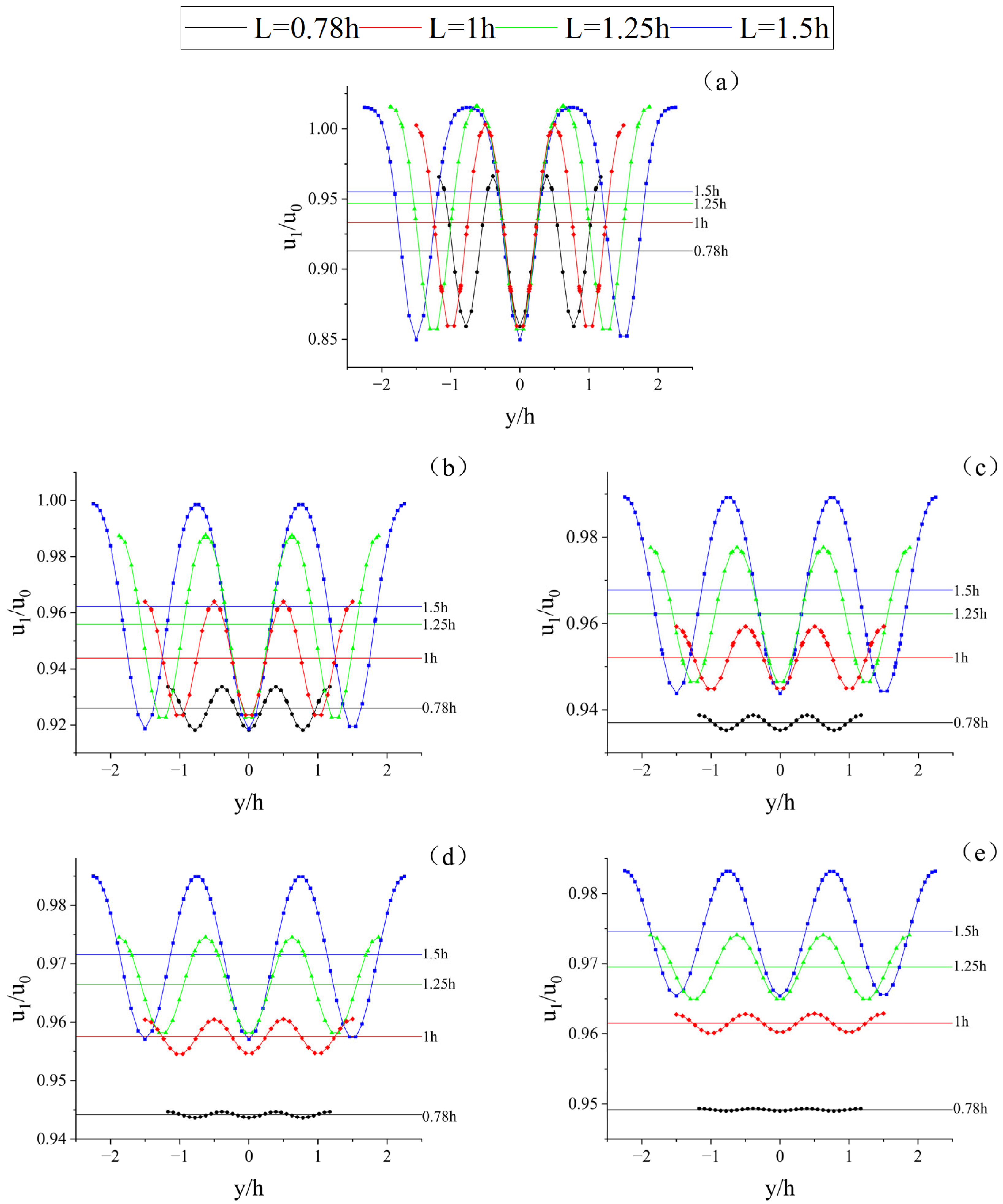
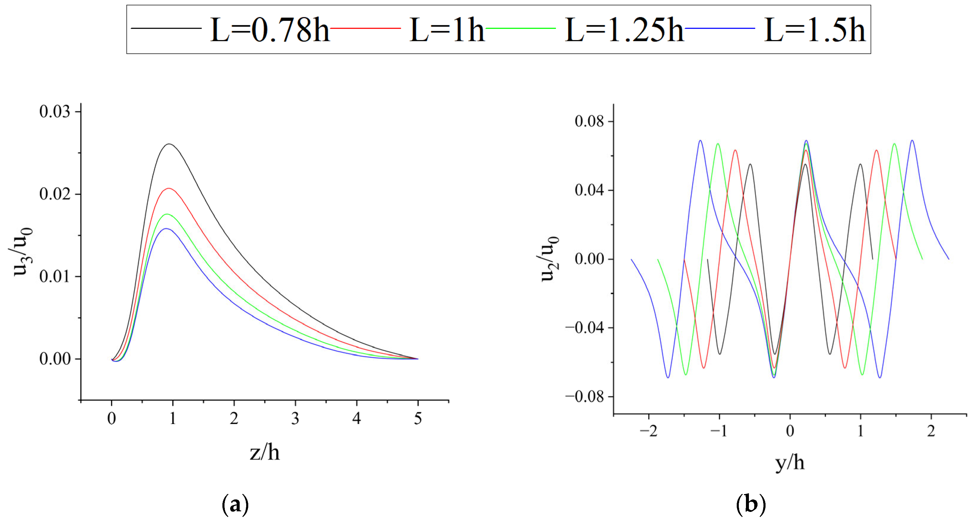
Figure 10 only shows the wind field information on the central axis behind the leeward side of the forest canopy, but considering the information on only one characteristic line is relatively one-sided. In order to obtain as much information as possible about the wind field, 1/2 of the height of the canopy was taken, and we extracted the variation in wind speed along the lateral direction at different distances from the leeward side of the forest belt with different spacings, as shown in Figure 11 and Figure 12. From Figure 13a, it can be seen that for a row of trees, each tree generates the lateral crosscurrent of equal magnitude and in the opposite direction. They cancel each other out at the split in the forest band, creating zones of high velocity on either side of the canopy, as shown in Figure 14. However, as the plant spacing decreases, the lateral crossflow is gradually suppressed, and there is more flow upward or through the canopy, as shown in Figure 13b, leading to an increase in velocity near the leeward side of the canopy. It is also because of the reduction in lateral crossflow velocity that the velocity at the forest belt slit will also decrease with decreasing plant spacing, which will also result in a slower velocity recovery on the leeward side of the plant, allowing for a more favorable average wind protection effectiveness and a longer protection distance.
Analyzing the fluctuation in velocity in the wind field and the change in its average velocity, it can be seen that the farther away from the forest belt, the average velocity on the leeward side of the forest belt with different spacing gradually increases, and the difference in the velocity between the leeward side of the canopy and the slit of the forest belt gradually decreases, which means that the stability of the wind field becomes more powerful. But the stability of the wind field is not only controlled by the distance from the leeward side of the forest belt; a reduction in the spacing of the forest belt will also lead to an increase in the stability of the wind field.
Also controlled by plant spacing and distance to the leeward side was the average velocity. In order to find the quantitative relationship between the average wind protection effectiveness of the forest belt and the plant spacing and distance from the leeward side, the plant spacing and the average wind protection effectiveness at different distances from the leeward side of the forest belt were fitted, and the relationship equation (Figure 15) between the average wind protection effectiveness and the plant spacing was obtained, as shown in Equation (9):
E = A D 1.05
where E is the average wind protection effectiveness on the leeward side of the forest belt, and the formula is shown in Equation (10). A is the parameter related to the distance from the leeward side of the forest belt, see Table 1. D is defined as dimensionless spacing (L/d).
E = 1 u 1 u 0
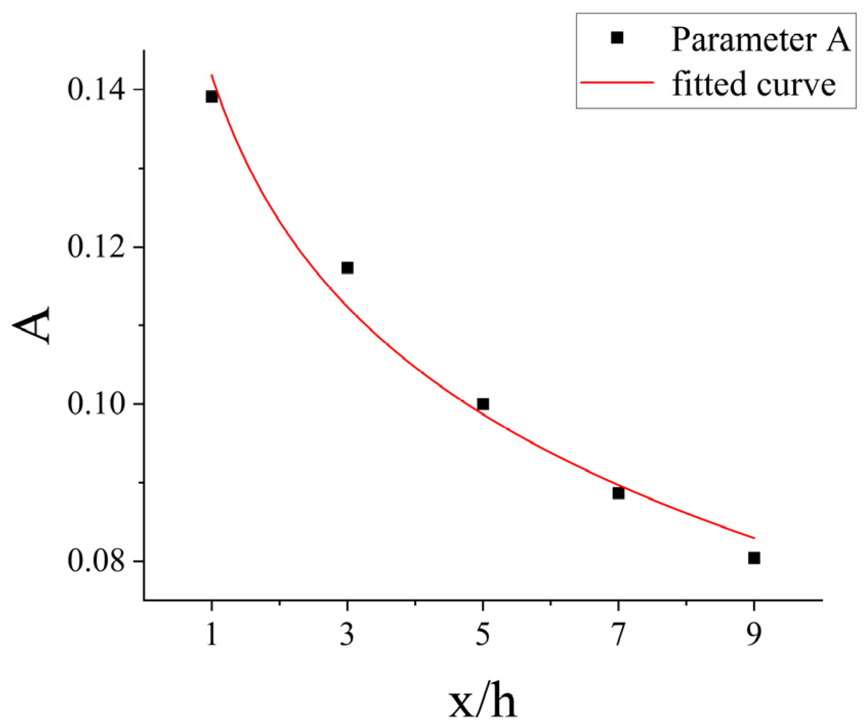
Fitting the distance to the leeward side of the forest belt to parameter A yields the following relationship (Figure 16):
A = 0 . 14184 0.0268 ln ( X )
where X represents the distance to the leeward side of the forest belt (x/h), and X > 0.25 when the characteristic point is outside the canopy, so the above equation is physically meaningful only when X > 0.25.
Combining Equations (9) and (11) yields an equation for the relationship between average wind protection effectiveness and plant spacing and distance from the leeward side of the forest belt:
E = 0.14184 0.0268 ln ( X ) D 1.05
The correlation factors of all the fitted formulas in this study are above 0.99, with high goodness of fit.

3.2.3. Influence of Solid Trunk on the Flow Field

To analyze the wind obstruction caused by the trunk, we focused on the half of the height of the trunk, as shown in Figure 17. Figure 18 shows the effect of forest belts with different spacings on the velocity at the tree trunk level; it can be seen that in the same way as in the canopy, within the height of the trunk as the plant spacing decreases, the average velocity of the whole wind field decreases, and the stability of the whole wind field is increased as the decrease in the plant spacing suppresses the lateral flow.
However, unlike the porous media canopy, the trunk has less influence on the wind field. From the lateral characterization line of the wind field, at 1 h on the leeward side, the velocity of the forest belt with a spacing of 1.5 h at the slit is hardly affected, which is caused by the shape of the model in this study (Figure 18a). In the design modeled here, the trunk is only 1/5 the diameter of the bottom of the canopy.
And, from the streamwise point of view, the velocity on the leeward side of the trunk recovered quite fast, and the velocity at 1 h on the leeward side of the trunk recovered to 85% of the incoming velocity, while the average velocity recovered to more than 98% of the incoming velocity. Interestingly, however, the average velocity of the wind field within the height of the trunk tends to decrease with increasing distance from the leeward side of the forest belt, which is very different from the porous media canopy.
This phenomenon also occurs precisely because of the differences between porous media and impenetrable solid exhibited in the wind field. We analyzed this distinction in detail in the previous section, at the same distance; the leeward side of the forest belt, within the height of the canopy, has a slower speed recovery and lower velocity, and within the height of the trunk, below, has a faster return of wind speed and higher velocity. The upper and lower layers are brought close to each other’s velocities by a constant exchange of momentum, and, finally, a log-law boundary layer flow is reestablished, so that the average velocity within the height of the canopy gradually increases, while the average velocity within the height of the trunk decreases gradually.

4. Conclusions

Under the plant canopy resistance factors taken and the plant shape conditions designed in this study, the one-row forest belt affected the wind profile up to 1.25-times of the tree height before the log-law boundary layer flow is reestablished, and the windbreaks with different spacing had basically the same effect on the wind profile, all of which restored the logarithmic law at 3 h on the leeward side. There are slight differences between the simulated and actual results in terms of horizontal wind speed trajectories. This could be attributed to the complexity of the canopy structure, as well as the limitations of the porous media model and the k-ε turbulence model in their applications. This is likely due to the presence of some unknown mechanisms in modeling the canopy structure, which indeed represents an interesting and worthwhile area for further research.
In addition, large-spaced vegetative shelterbelts provide greater protection in the near-wake region, while small-spaced forest belts are more effective at reducing wind speed in the recirculation zone. As for the average velocity of the wind field, the smaller the plant spacing is, the stronger weakening effect. Based on the simulation results of several cases, a parameterization scheme of the average wind protection effectiveness with respect to the plant spacing and the distance from the leeward side of the plant shelterbelt is given. In arid and semi-arid regions, the scarcity of water resources has always been an issue in the construction and maintenance of windbreaks. Our research aims were to plant the minimum number of trees to achieve the maximum effect of wind prevention and sand fixation. The environmental conditions and expectations for windbreaks vary from one region to another, and the proposed relationship will assist foresters in selecting appropriate planting distances based on their specific needs. For instance, if someone wants to reduce the wind speed within 3 h on the leeward side to below 95% of the incoming wind speed, they should choose a plant spacing of 2 d for the windbreak. The windbreak designed in this study is a single row, but our research can provide insights for multiple-row windbreaks as well. However, one limitation is that the drag coefficient and incoming wind speed are fixed in our study, which poses significant constraints in practical applications. So, further research is needed to address different tree species and various wind field environments.
From the results of the simulation, there is a big difference in the weakening effect of the canopy and the trunk from the comparison of their velocity; this is evidenced by the fact that the distance that the wind velocity passing through the canopy recovers to the incoming velocity is longer, while the wind velocity passing through the trunk recovers faster. Therefore, it is recommended that a row of shrubs be planted before and after the tree forest belt to reduce the near-surface velocity in actual engineering practice.

Author Contributions

Supervision, N.H. and J.Z.; designed the study, Y.Z. and K.Z.; methodology, J.Z., Y.Z. and J.S.; software, Y.Z., X.L. and B.H.; writing—original draft, Y.Z.; writing—review and editing, J.Z., J.S. and Y.Z. All authors have read and agreed to the published version of the manuscript.

Funding

This research was funded by the National Natural Science Foundation of China (grant nos. 41931179, 42376232), National key research and development program (2023YFF1304203), the Second Tibetan Plateau Scientific Expedition and Research Program (grant no. 2019QZKK020611) and the Key Subjects of Science and Technology Development Program of China Railway Engineering Design and Consulting Group Co., Ltd. (Research-2019-62).

Institutional Review Board Statement

Not applicable.

Informed Consent Statement

Not applicable.

Data Availability Statement

The data presented in this study are available on request from the corresponding author. The data are not publicly available due to privacy.

Conflicts of Interest

Author Xuanmin Li and Bin Han were employed by the company China Railway Engineering Design and Consulting Group Co., Ltd. The remaining authors declare that the research was conducted in the absence of any commercial or financial relationships that could be construed as a potential conflict of interest.

References

  1. Li, S.Y.; Tang, Q.L.; Lei, J.Q.; Xu, X.W.; Jiang, J.; Wang, Y.D. An overview of non-conventional water resource utilization technologies for biological sand control in Xinjiang, northwest China. Environ. Earth Sci. 2015, 73, 873–885. [Google Scholar] [CrossRef]
  2. Li, H.L.; Wang, Y.D.; Li, S.Y.; Askar, A.; Wang, H.F. Shelter Efficiency of Various Shelterbelt Configurations: A Wind Tunnel Study. Atmosphere 2022, 13, 1022. [Google Scholar] [CrossRef]
  3. Yang, W.B.; Li, W.; Dang, H.Z.; Feng, W.; Lu, Q.; Jiang, L.N.; Yang, H.Y.; Wu, X.Q. Desertification Control with Low Coverage Vegetation—Principles, Models and Effects; Science Press: Beijing, China, 2016; pp. 316–320. [Google Scholar]
  4. Cornelis, W.M.; Gabriels, D. Optimal windbreak design for wind-erosion control. J. Arid. Environ. 2005, 61, 315–332. [Google Scholar] [CrossRef]
  5. Cheng, H.; He, W.W.; Liu, C.C.; Zou, X.Y.; Kang, L.Q.; Chen, T.; Zhang, K. Transition model for airflow fields from single plants to multiple plants. Agric. For. Meteorol. 2019, 266, 29–42. [Google Scholar] [CrossRef]
  6. Mayaud, J.R.; Wiggs, G.F.; Bailey, R.M. Characterizing turbulent wind flow around dryland vegetation. Earth Surf. Process. Landf. 2016, 41, 1421–1436. [Google Scholar] [CrossRef]
  7. Okin, G.S. A new model of wind erosion in the presence of vegetation. J. Geophys. Res. Earth Surf. 2008, 113, 758. [Google Scholar] [CrossRef]
  8. Cheng, H.; Liu, C.; Kang, L. Experimental study on the effect of plant spacing, number of rows and arrangement on the airflow field of forest belt in a wind tunnel. J. Arid. Environ. 2020, 178, 104169. [Google Scholar] [CrossRef]
  9. Dong, Z.B.; Luo, W.Y.; Qian, G.Q.; Wang, H.T. A wind tunnel simulation of the mean velocity fields behind upright porous fences. Agric. For. Meteorol. 2007, 146, 82–93. [Google Scholar] [CrossRef]
  10. Svensson, U.; Häggkvist, K. A two-equation turbulence model for canopy flows. J. Wind. Eng. Ind. Aerodyn. 1990, 35, 201–211. [Google Scholar] [CrossRef]
  11. Gash, J.H.C. Observations of turbulence downwind of a forest-heath interface. Boundary-Layer Meteorol. 1986, 36, 227–237. [Google Scholar] [CrossRef]
  12. Wu, T.G.; Yu, M.K.; Wang, G.; Wang, Z.X.; Duan, X.; Dong, Y.; Cheng, X.Y. Effects of stand structure on wind speed reduction in a Metasequoia glyptostroboides shelterbelt. Agrofor. Syst. 2013, 87, 251–257. [Google Scholar] [CrossRef]
  13. Wu, X.X.; Zou, X.Y.; Zhou, N.; Zhang, C.L.; Shi, S. Deceleration efficiencies of shrub windbreaks in a wind tunnel. Aeolian Res. 2015, 16, 11–23. [Google Scholar] [CrossRef]
  14. Rosenfeld, M.; Marom, G.; Bitan, A. Numerical simulation of the airflow across trees in a windbreak. Boundary-Layer Meteorol. 2010, 135, 89–107. [Google Scholar] [CrossRef]
  15. Sogachev, A.; Panferov, O. Modification of two-equation models to account for plant drag. Boundary-Layer Meteorol. 2006, 121, 229–266. [Google Scholar] [CrossRef]
  16. Santiago, J.L.; Martin, F.; Cuerva, A.; Bezdenejnykh, N.; Sanz-Andrés, A. Experimental and numerical study of wind flow behind windbreaks. Atmos. Environ. 2007, 41, 6406–6420. [Google Scholar] [CrossRef]
  17. Wilson, J.D.; Yee, E. Calculation of winds disturbed by an array of fences. Agric. For. Meteorol. 2003, 115, 31–50. [Google Scholar] [CrossRef]
  18. Packwood, A.R. Flow through porous fences in thick boundary layers: Comparisons between laboratory and numerical experiments. J. Wind. Eng. Ind. Aerodyn. 2000, 88, 75–90. [Google Scholar] [CrossRef]
  19. Mochida, A.; Tabata, Y.; Iwata, T.; Yoshino, H. Examining tree canopy models for CFD prediction of wind environment at pedestrian level. J. Wind. Eng. Ind. Aerodyn. 2008, 96, 1667–1677. [Google Scholar] [CrossRef]
  20. Endalew, A.M.; Hertog, M.; Delele, M.A.; Baetens, K.; Persoons, T.; Baelmans, M.; Verboven, P. CFD modelling and wind tunnel validation of airflow through plant canopies using 3D canopy architecture. Int. J. Heat Fluid Flow 2009, 30, 356–368. [Google Scholar] [CrossRef]
  21. Heisler, G.M.; Dewalle, D.R. Effects of windbreak structure on wind flow. Agric. Ecosyst. Environ. 1988, 22, 41–69. [Google Scholar] [CrossRef]
  22. Perera, M.D.A.E.S. Shelter behind two-dimensional solid and porous fences. J. Wind. Eng. Ind. Aerodyn. 1981, 8, 93–104. [Google Scholar] [CrossRef]
  23. Skidmore, E.L.; Hagen, L.J. Evapotranspiration and the Aerial Environment as Influenced by Windbreaks; Springer: Berlin/Heidelberg, Germany, 1970. [Google Scholar]
  24. Launder, B.E.; Spalding, D.B. The numerical computation of turbulent flows. In Numerical Prediction of Flow, Heat Transfer, Turbulence and Combustion; Pergamon: Berlin, Germany, 1983; pp. 96–116. [Google Scholar]
  25. Liu, C.C.; Zheng, Z.Q.; Cheng, H.; Zou, X.Y. Airflow around single and multiple plants. Agric. For. Meteorol. 2018, 252, 27–38. [Google Scholar] [CrossRef]
  26. Blocken, B.; Carmeliet, J.; Stathopoulos, T. CFD evaluation of wind speed conditions in passages between parallel buildings—Effect of wall-function roughness modifications for the atmospheric boundary layer flow. J. Wind. Eng. Ind. Aerodyn. 2007, 95, 941–962. [Google Scholar] [CrossRef]
  27. Leenders, J.K.; Boxel, J.H.; Sterk, G. The effect of single vegetation elements on wind speed and sediment transport in the Sahelian zone of Burkina Faso. Earth Surf. Process. Landf. J. Br. Geomorphol. Res. Group 2007, 32, 1454–1474. [Google Scholar] [CrossRef]
  28. Ma, R.; Wang, J.; Qu, J.; Liu, H. Effectiveness of shelterbelt with a non-uniform density distribution. J. Wind. Eng. Ind. Aerodyn. 2010, 98, 767–771. [Google Scholar] [CrossRef]
  29. Judd, M.J.; Raupach, M.R.; Finnigan, J.J. A wind tunnel study of turbulent flow around single and multiple windbreaks, part I: Velocity fields. Boundary-Layer Meteorol. 1996, 80, 127–165. [Google Scholar] [CrossRef]
  30. Raupach, M.R.; Finnigan, J.J.; Brunet, Y. Coherent eddies and turbulence in vegetation canopies: The mixing-layer analogy. Boundary-Layer Meteorology 25th Anniversary Volume, 1970–1995: Invited Reviews and Selected Contributions to Recognise Ted Munn’s Contribution as Editor over the Past 25 Years; Springer: Berlin/Heidelberg, Germany, 1996; pp. 351–382. [Google Scholar]
  31. Van, E.J.; Karschon, R.; Razumova, L.A.; Robertson, G.W. Windbreaks and shelterbelts. World Meteorological Orgabization, Commission for Agricultural Meteorology; World Meteorological Organization: Geneva, Switzerland, 1964; p. 188. [Google Scholar]
Figure 1. Comparison of flow fields on the leeward side of the canopy between porous media and impenetrable solid: (a) impenetrable solid; (b) porous media.
Atmosphere 15 00602 g001
Figure 2. Numerical simulation comparison with actual measurements [25].
Atmosphere 15 00602 g002
Figure 3. Computational domain and plant model dimensions.
Atmosphere 15 00602 g003
Figure 4. Flow field distribution near the canopy of a single plant: (a) airflow on the windward side of the canopy (the red arrows indicate the blood flow, the green arrows indicate the lateral cross flow and the blue arrows indicate the vertical cross flow); (b) the x-component velocity variations (y = 0, z = 0.5 h); (c) the y-component velocity variations (x = 0, z = 0.5 h); (d) the z-component velocity variations (x = −0.5 h, y = 0).
Atmosphere 15 00602 g004aAtmosphere 15 00602 g004b
Figure 5. The pressure distribution in the vertical plane at y = 0.
Atmosphere 15 00602 g005
Figure 6. The x-component velocity distribution of the flow field: (a) on the vertical plane y = 0; (b) on the horizontal plane z = 0.5 h.
Atmosphere 15 00602 g006aAtmosphere 15 00602 g006b
Figure 7. Velocity variation distribution along streamwise in the vertical plane at the center of the forest belt (y = 0, z/h = 0–2).
Atmosphere 15 00602 g007
Figure 8. Comparison of the vertical velocity profiles above plants calculated in this study with past results (normalizing velocity scales are the mean velocity uh at the canopy top).
Atmosphere 15 00602 g008
Figure 9. Coordinate system and analysis location (the red line represents the analyzed characteristic line).
Atmosphere 15 00602 g009
Figure 10. Velocity variation on the leeward side of the center of the forest belt at different spacing along the streamwise direction.
Atmosphere 15 00602 g010
Figure 11. Within the height of the canopy characteristic line selection location (1/2 of the height of the canopy).
Atmosphere 15 00602 g011
Figure 12. This text describes the variation in velocity and average velocity on the characteristic line at different distances from the leeward side of the canopy of a forest belt. Distance to leeward side: (a) 1 h; (b) 3 h; (c) 5 h; (d) 7 h; (e) 9 h, where the straight line represents the average velocity.
Atmosphere 15 00602 g012
Figure 13. Variations in velocity at different plant spacings: (a) the y-component velocity variations; (b) the z-component velocity variations.
Atmosphere 15 00602 g013
Figure 14. The x-component velocity distribution in the horizontal plane for a forest belt with a spacing of 0.78 h (z = 0.5 h).
Atmosphere 15 00602 g014
Figure 15. Relationship between plant spacing and the wind protection effectiveness at different distances on the leeward side. Distance to leeward side: (a) 1 h; (b) 3 h; (c) 5 h; (d) 7 h; (e) 9 h.
Atmosphere 15 00602 g015
Figure 16. Relationship between the distance to the leeward side of the forest belt and parameter A.
Atmosphere 15 00602 g016
Figure 17. Within the height of the trunk characteristic line selection location (1/2 of the height of the trunk).
Atmosphere 15 00602 g017
Figure 18. This text describes the variation in velocity and average velocity on the characteristic line at different distances from the leeward side of the trunk of a forest belt. Distance to leeward side: (a) 1 h; (b) 3 h; (c) 5 h; (d) 7 h; (e) 9 h, where the straight line represents the average velocity.
Atmosphere 15 00602 g018
Table 1. Variation in parameter A at different distances from the leeward side of the forest belt.
Leeward DistanceParameter A
1 h0.13912
3 h0.11737
5 h0.10001
7 h0.08868
9 h0.0804
Disclaimer/Publisher’s Note: The statements, opinions and data contained in all publications are solely those of the individual author(s) and contributor(s) and not of MDPI and/or the editor(s). MDPI and/or the editor(s) disclaim responsibility for any injury to people or property resulting from any ideas, methods, instructions or products referred to in the content.