Observation-Based Ozone Formation Rules by Gradient Boosting Decision Trees Model in Typical Chemical Industrial Parks

Abstract

Ozone pollution in chemical industrial parks is severe and complicated and is significantly influenced by pollutant emissions and meteorological parameters. In this study, we innovatively investigated the formation rules of ozone by using observation-based analyses and a gradient-boosting decision tree (GBDT) model, focusing on a typical chemical industrial park located in the Yangtze River Delta of China. The results revealed that ozone concentration was positively correlated with temperature while negatively correlated with NO₂ concentration and relative humidity (RH). Ozone pollution was predominantly observed from April to October (M_4–10). The optimized GBDT model was subsequently utilized to establish a specific and quantifiable relationship between each single dominant impact factor (RH, NO₂, temperature, and PM_2.5) and ozone within a complex and uncertain multi-factor context during M_4–10. Detailed discussions were conducted on the reaction rate of ozone-related to different levels of RH and temperature. The accumulation of ozone was favored by high temperature and low RH, with the maximum ozone concentration observed at the RH of 50% and the temperature of 35 °C. The NO₂-O₃ change curve exhibited distinct phases, including a period of stability, gradual increase, rapid increase, and equilibrium. During the second and third periods, the ratio of ozone production to NO₂ consumption was 0.10 and 2.73, respectively. Furthermore, there was a non-monotonic relationship between variations in ozone concentration and PM_2.5 concentration. Hence, it is imperative to implement fine control strategies in the park, such as adopting seasonal production strategies, implementing targeted measures for controlling NO_x and active VOCs, and employing special control methods during periods of high temperature. This study provides aid in achieving effective management of localized ozone pollution and ensuring compliance with air quality standards.

1. Introduction

As factories retreat from cities to industrial parks, centralized emissions from chemical industrial parks greatly affect the surrounding air quality [1,2]. Due to the massive emission of VOCs and NO_x from chemical industries, ozone pollution has become one of the most prominent problems and has caused increasing concern in human society [3,4,5,6]. High ozone concentrations can affect human health, plant growth, and climate change [7,8,9]. As a secondary pollutant, surface ozone is generated by complex photochemical reactions of multiple precursors under solar radiation [10,11,12,13].

Previously, extensive research has been conducted on the ozone formation rules in large-scale areas such as cities. However, in recent years, there has been a growing research focus on small-scale areas, especially chemical industrial parks [14,15,16,17]. With concentrated pollution sources, high pollutant concentrations, and complex pollutant compositions, chemical industrial parks show more confusing ozone formation rules than urban areas. The complicated production conditions cause ozone pollution in industrial parks, not to mention the variable meteorological parameters [18,19,20]. One study found that the offshore petrochemical industrial park is responsible for most VOC emissions in the surrounding environment, and its impact on local ozone level is significant. Additionally, the total amount of local ozone and its precursors were generally constant [21]. Another study has revealed that air pollutants, especially ozone from industrial parks, will be transported to stadiums during the 2022 Asian Games, which could significantly impact the air quality of important activities [22]. Other researchers concentrated on sensitivity analysis [23], pollution event analysis [24], and formation rules research [16] related to ozone. Therefore, it is extremely important to explore ozone formation rules in chemical industrial parks.

The complex photochemical reactions of ozone lead to a highly nonlinear relationship between ozone and its impact factors [25,26]. Observation-based research has led to some progress in determining the ozone formation rules, which can adapt to various scenarios and obtain relatively apparent regularity between ozone level and impact factors. A detailed study found that high concentrations of precursors, high temperature, low relative humidity (RH), and moderate high wind speeds (WS) were conducive to generating urban ozone episodes in Zhengzhou [26]. The authors studied the impact of meteorological factors on pollutants and found that temperature had the greatest effect on ozone [27]. Another interesting study revealed a strong correlation between ozone and meteorology, with wind speed (WS) and wind direction (WD) primarily contributing to the transport and mixing of precursors, while temperature directly influenced ozone formation [28]. Some researchers evaluated the long-term trend of ozone level and found that the decline of MDA8 from 2007 to 2014 was associated with CO and NO_x, while the increase in ozone level from 2015 to 2021 was linked to NO_x emissions [29]. Another investigation focused on the trend of ambient ozone level and its associations with precursor gases and meteorology using ground and satellite observations. It concluded that reduced NO₂ concentration improved O₃ air quality, but local meteorology conditions worsened it [30]. However, it is difficult to recognize the effects of these factors without obvious rules for ozone formation or distinguish the contribution of different impact factors based on observation analyses.

Therefore, some more complicated approaches have also been applied to reveal the ozone formation rules, such as the Empirical Kinetics Modeling Approach (EKMA), chemical transport models, and machine learning. EKMA can only reflect the relationship between ozone and the precursors under certain initial conditions, but it cannot adapt to changes in the nonlinear relationship caused by dynamic changes in precursors concentration and meteorological parameters under realistic conditions [31]. Air quality models require considerable data input and expensive computational costs, which limit their applicability [32,33,34,35].

Machine learning is widely used in the field of air pollution, and it can use even irregular data to determine internal mechanisms and obtain high prediction accuracy with cheaper computational cost [35,36,37]. Several machine-learning models have been used to estimate ozone concentrations. Some authors used linear regression and the random forest model to fit historical data from monitoring of ozone concentrations, and the results showed that sunlight, NO₂, WS, and NO were the most important factors leading to heavy ozone pollution [18]. A study was conducted to establish an artificial neural network (ANN) to investigate the ozone formation rules. The findings indicated that the studied area belonged to the NO_x-sensitive regime, with sensitivity strongly affected by relative humidity (RH) and pressure (P) [16]. The spatiotemporal characteristics of ground-level O₃ were investigated in another study using ground observations and satellite retrievals with interpretable machine learning models, highlighting the significant influence of temperature, RH, total column O₃, as well as the distributions and interactions of precursors on the observed patterns of O₃ in Zhejiang [38]. The ozone concentration prediction was successfully achieved by employing a deep convolutional neural network (CNN) that integrated meteorological data and air pollution concentrations, yielding promising outcomes in an intriguing study [39]. The estimation of O₃ in Beijing was conducted using a Random Forest model, revealing that land surface temperature and temperature at 2 m above the surface emerged as the most influential factors while NO₂ stood out as the highest influencing factor among the air quality parameters [40]. Moreover, the gradient-boosting decision tree (GBDT) is another popular and powerful machine learning algorithm that exhibits great performance in interpretability, accuracy, and efficiency while learning with big data [41,42]. In addition, it also performs well for complex correlated variables with greater robustness and generalization, which is suitable for the fitting of ozone levels influenced by multiple factors [43,44].

Therefore, this study explored the temporal variations and observation-based correlations based on ozone concentration together with those of 6 other atmospheric pollutants and 5 meteorological parameters. Then, the GBDT model was innovatively employed to discover the ozone formation rules for the high ozone pollution period. Furthermore, the optimized model was utilized to establish a specific and quantifiable relationship between an individual impact factor and ozone within a complex and uncertain multi-factor context. This work aids in realizing small-scale ozone pollution control and meeting air quality standards.

2. Methodology

2.1. Study Area

A typical chemical industrial park [45,46] located in the southern Yangtze River Delta, northeastern Zhejiang Province (30.61° N, 121.07° E), and adjoining Hangzhou Bay was selected as depicted in Figure 1. It is the only outlet and foreign trade channel for northern Zhejiang Province with a superior geographical position and convenient waterway transportation. With a humid subtropical monsoon climate, this park has four distinct seasons. In addition, 65.7% of factories in this park produce new chemical materials, which has formed several industrial chains with competitiveness, including polycarbonate, silicone, ethylene oxide, Purified Terephthalic Acid (PTA), and so on. Adjacently distributed industrial sources with high and intermittent levels of pollutant emission, as well as mobile sources that serve the transportation industry that drives the production of parks, are the main sources of pollutant emission in parks.

2.2. Datasets

Monitoring data of atmospheric pollutants and meteorological parameters mainly came from the automatic environmental air monitoring station placed in the park.

Table 1. The monitoring information for atmospheric pollutants and meteorological parameters.

Monitoring Parameters		Detection Method	Detection Limitation/ Precision	Data Collected Spans	Temporal Resolution
Atmospheric pollutants	O3	absorption spectrophotometry	0.05 ppb	January 2014~December 2018	1 h
	NOx	chemiluminescence	0.4 ppb	January 2014~December 2018	1 h
	SO2	ultraviolet fluorescence	0.5 ppb	January 2014~December 2018	1 h
	CO	gas filter correlation analysis	0.04 ppm	January 2014~December 2018	1 h
	PM2.5	β-ray turbidity	4 μg·m−3	January 2015~December 2018	1 h
	VOCs	gas chromatography-mass spectrometry	0.15 ppb	January 2018~December 2018	1 h
Meteorological parameters	Temperature	NTC negative temperature coefficient thermistor	±0.2 °C	January 2018~December 2018	1 h
	RH	Capacitive sensing	±2% RH	January 2018~December 2018	1 h
	P	MEMS Capacitive sensing	±0.5 hPa	January 2018~December 2018	1 h
	WS	ultrasonic wave	±0.3 m/s	January 2018~December 2018	1 h
	WD	ultrasonic wave	RMSE < 3° (>1.0 m/s)	January 2018~December 2018	1 h

displayed the detailed monitoring information for all the monitoring parameters. The concentration of ozone was detected by ultraviolet absorption spectrophotometry with a limit of detection of 0.05 ppb. SO₂ was detected by the pulsed ultraviolet fluorescence method, and the detection limit was 0.5 ppb. The chemiluminescence method was used to quantify NO_x (including NO and NO₂) with a detection limit of 0.4 ppb. CO was detected by the gas filter correlation analysis method with a detection limit of 0.04 ppm. Fine particle matter (PM_2.5) was analyzed by the β-ray turbidity method with a limit of detection of 4 μg·m⁻³. VOCs were analyzed by gas chromatography-mass spectrometry with flame ionization detection, and the limit of detection was 0.15 ppb. The VOCs monitored mainly involved 5 categories: alkanes (24 species), alkenes (10 species), ethyne, aromatics (14 species), and halocarbons (21 species), as shown in Table S1. Meteorological parameters were monitored by the WS500-UMB weather system, which included temperature, RH, atmospheric pressure (P), WS, and wind direction (WD).

2.3. Pearson Correlation Coefficient

The Pearson correlation coefficient is a statistical parameter that quantitatively measures the correlation between two variables [47,48,49]. It can be calculated as in Equation (1):

$$\rho (x,y)=\frac{{\displaystyle {\sum }_{i=1}^n(x_i-\overline{x})(y_i-\overline{y})}}{\sqrt{{\displaystyle {\sum }_{i=1}^n{(x_i-\overline{x})}^2{\displaystyle {\sum }_{i=1}^n{(y_i-\overline{y})}^2}}}}$$

(1)

where x_i and y_i are the values of variables x and y at i o’clock, and $\overline{x}$ and $\overline{y}$ are the average values of the x and y variables, respectively.

2.4. GBDT Model

The GBDT model is one of the most powerful learning algorithms based on decision trees and solves the overfitting defect of a single decision tree to a certain extent. The main advantage is similar to that of other models based on decision trees; these algorithms perform well with heterogeneous features without scaling the data. The key of the GBDT model is to optimize a cost function over function space by iteratively choosing a function (weak hypothesis) that points in the negative gradient direction, that is, an algorithm that uses the value of the negative gradient of the loss function in the current model as the approximate residual in the lifting tree algorithm to fit a lifting tree and minimize the loss function by gradually reducing the residual.

2.4.1. Algorithm

The detailed algorithm is described as follows [42,50].

First, the training data D = {(x_i, y_i)} (i = 1, 2,…, N) was built by setting the impact factors as the independent variable dataset and ozone concentration as the dependent variable dataset. The prediction function f(x) was simulated by the GBDT model, and the loss function was defined as L(y, f(x)). Specifically, the GBDT model was applied based on the following algorithm:

(1)

The model was initialized with constants c to minimize the loss function as in Equation (2):

$$f_0(x)=\arg \underset{c}{\min }{\displaystyle {\sum }_{i=1}^{N}L(y_i,c)}$$

(2)

(2)

For the mth regression trees, m = 1, 2, …, M.

(a)

For the ith variable, i = 1, 2, …, N, the value of the negative gradient of the loss function was calculated based on the current model f_m-1(x) according to Equation (3) and taken as the approximate value of the residual error.

$$r_{mi}=-{\left[\frac{\partial L(y_i,f(x_i))}{\partial f(x_i)}\right]}_{f(x_i)=f_{m-1}(x)}$$

(3)

(b)

Then, a regression tree was fitted to r_mi to obtain the leaf node area R_mj of the jth leaf node in the mth tree, j = 1, 2, …, J.

(c)

For the jth leaf node, a linear search was used to estimate the values of the leaf node areas to minimize the loss function value, as shown in Equation (4):

$$c_{mj}=\arg \underset{c}{\min }{\displaystyle {\sum }_{x_i\in R_{mj}}L(y_i,f_{m-1}(x_i)+c)}$$

(4)

(d)

The regression tree was updated as in Equation (5):

$$f_m(x)=f_{m-1}(x)+{\displaystyle {\sum }_{j=1}^J{c}_{mj}I(x\in R_{mj})}$$

(5)

(3)

Finally, the final regression model was obtained as in Equation (6):

$$\stackrel{\wedge }{f}(x)=f_M(x)+{\displaystyle {\sum }_{m=1}^M{\displaystyle {\sum }_{j=1}^J{c}_{mj}I(x\in R_{mj})}}$$

(6)

A grid search was used to determine the best parameters for the GBDT model. Grid search is a method based on the exhaustive search method, and the best learning algorithm is obtained by optimizing the parameters of the estimated function through cross-validation. Cross-validation randomly divides the entire model-fitting dataset into k (k = 10 in this study) mutually exclusive subsets of similar size [51]. Then, k-1 subsets are used each time as the training set to fit the model, and the remaining subsets are used as the testing set to make predictions. In this way, the model is trained and tested k times until every subset is predicted, which effectively suppresses the overfitting of the model and identifies the best parameters.

2.4.2. Operation Framework

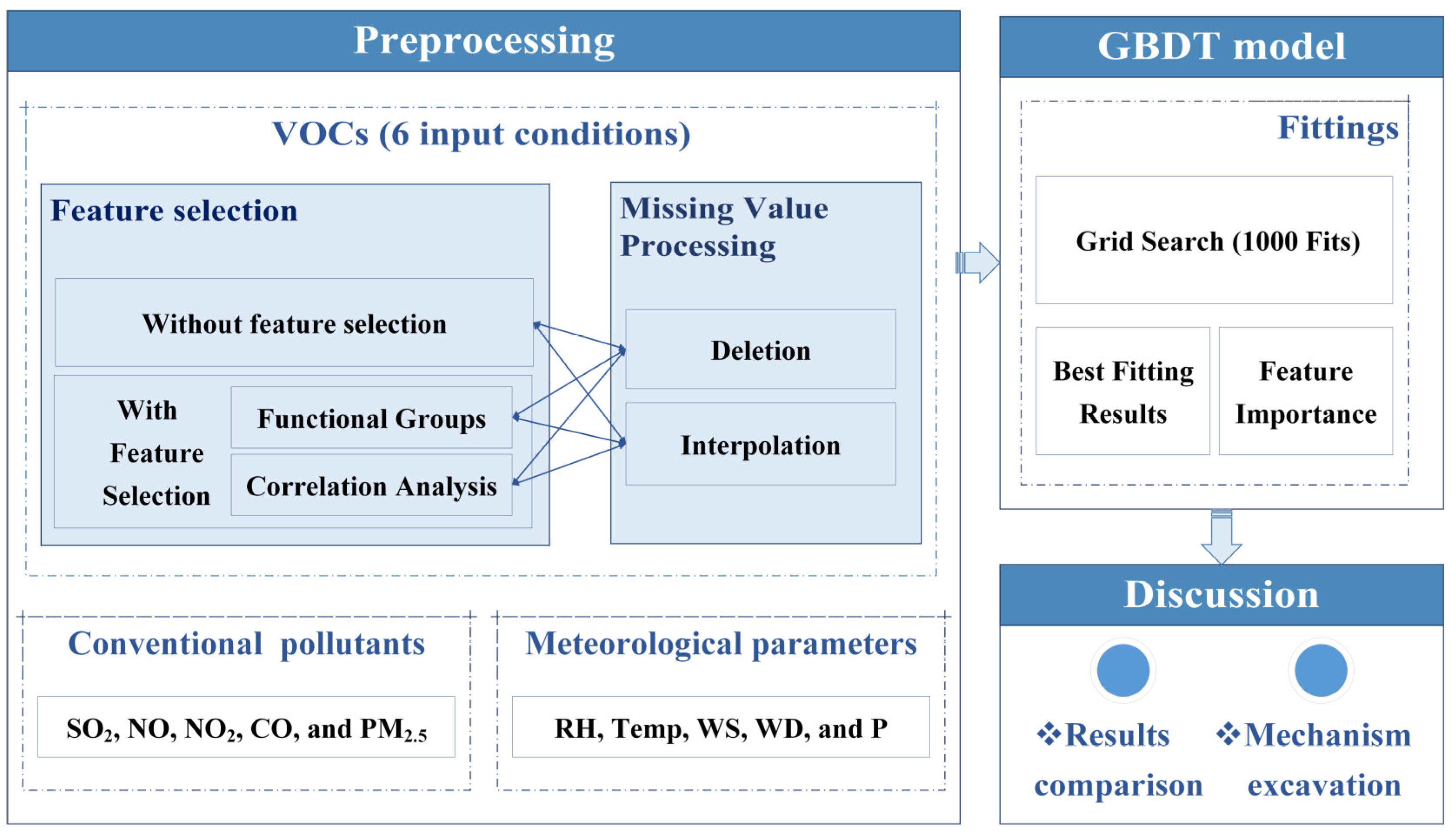
The implementation of this model was carried out using the Python programming language. The model operation framework for fitting the ozone concentration data is shown in Figure 2. The input data was preprocessed based on the hourly data, and the input conditions were established according to different settings for feature selection and missing value processing. The GBDT model was then trained on the preprocessed M_4–10 data, with a training-to-testing set ratio of 7:3. Based on the fitting results, further work was undertaken to develop a deeper understanding of the ozone formation rules.

2.4.3. Preprocessing

Since the effectiveness of some features can be partially predicted and the VOC composition is too complex, the level of conventional atmospheric pollutants (SO₂, NO, NO₂, PM_2.5, CO) and meteorological parameters (temperature, RH, P, WS, WD) were fixedly selected, but VOCs were selected based on different criteria when fitting the GBDT model. The feature selection process is effective in reducing the algorithm’s running time and increasing the interpretability of the model. The FILTER method, which selected features before model fitting, was used for feature selection. Classification and correlation analyses realized feature selection with different considerations. The former is based on functional groups to divide VOCs into 4 categories (alkanes, alkenes and ethyne, aromatics and halocarbons) to reduce the instability caused by missing values of some VOC concentrations, which can reflect the influence of VOC species with similar reaction mechanisms. The latter consideration, which is based on the Pearson correlation coefficient, can determine the impacts of VOC species with identical sources or other relationships on ozone formation to reduce the interference of collinearity with the model. As described specifically in the Supplementary Material in Text S1 and Figure S6, eleven VOC species were ultimately selected for model fittings. Moreover, in case key information on VOCs was lost or the accuracy of the model was reduced, the GBDT model was also performed without feature selection. That is, all VOC species were selected indiscriminately. In contrast, the complexity of the model with feature selection was largely reduced compared with the model without feature selection.

In addition, the missing values were processed by both deletion and interpolation. Deleting missing values leads to a smaller training set, while interpolation may cause distortion of some data, and a single method may cause the model to deviate from the real situation. Hence, the results of these two processing methods were considered together in cases of nonnegligible deviation.

Finally, the combined feature selection and missing value process was used to establish 6 input conditions for each fitting to obtain a more reasonable and reliable simulation.

2.5. Model Performance Indices

To evaluate the model performance, the coefficient of determination (R²) and the root mean square error (RMSE) were calculated [18]. As shown in Equation (7), R² measures the proportion of variation in the dependent variable that can be explained by the independent variable. At the same time, MSE represents the square of the difference between the true value and the predicted value, as shown in Equation (8).

$$R^2=1-\frac{{\displaystyle {\sum }_{i=1}^n(\stackrel{\wedge }{f}(x_i)-\overline{y}{)}^2}}{{\displaystyle {\sum }_{i=1}^n{(y_i-\overline{y})}^2}}$$

(7)

$$RMSE=\sqrt{\frac{{\displaystyle {\sum }_{i=1}^n(y_i-\stackrel{\wedge }{f}(x_i){)}^2}}{n}}$$

(8)

3. Results

3.1. Temporal Variation in Atmospheric Pollutants and Meteorological Parameters

The annual average concentrations for 6 conventional atmospheric pollutants were determined from 2014 to 2018. Figure S1 in the Supplementary Materials demonstrates that the levels of SO₂, NO, NO₂, and CO all met the Grade (I) National Ambient Air Quality Standard (NAAQS) (GB3095-2012) [52], and the concentrations changed slightly in different years. The concentration of PM_2.5 decreased year by year, but it still exceeded Grade (Ⅱ) of NAAQS (GB3095-2012). More seriously, ozone concentrations have reached a high level in recent years, which requires more attention to improving the air quality in parks.

Considering the loss of historical monitoring data of VOC concentration, this study focused on the online monitoring data in 2018 for further analysis.

3.1.1. Conventional Atmospheric Pollutants

The temporal variations and average monthly variations in O₃, SO₂, NO, NO₂, CO, and PM_2.5 levels in 2018 are shown in Figures S2 and S3, respectively. The annual average ozone concentration was 73 μg·m⁻³, July was the month with the maximum hourly ozone concentration of 340 μg·m⁻³, and June was the month with the largest monthly average ozone concentration of 105 μg·m⁻³. The ozone concentrations exhibited higher values during the period from April to October (M_4–10) compared to other months. In addition, statistical analysis showed that M_4–10 was also the period with high incidences of heavy ozone pollution with a frequency of 96.7%. The concentration of SO₂ was significantly larger in the first semi-year than in the second semi-year, with an average value of 9 μg·m⁻³. The NO concentration was stable at approximately 3 μg·m⁻³ throughout the year and showed little small variation. In addition, the monthly concentrations of NO₂, CO, and PM_2.5 showed single valleys in June, July, and August, which were opposite those of ozone. The average annual concentrations of NO₂, CO and PM_2.5 were 26 μg·m⁻³, 0.689 mg·m⁻³, and 35 μg·m⁻³ in 2018, respectively.

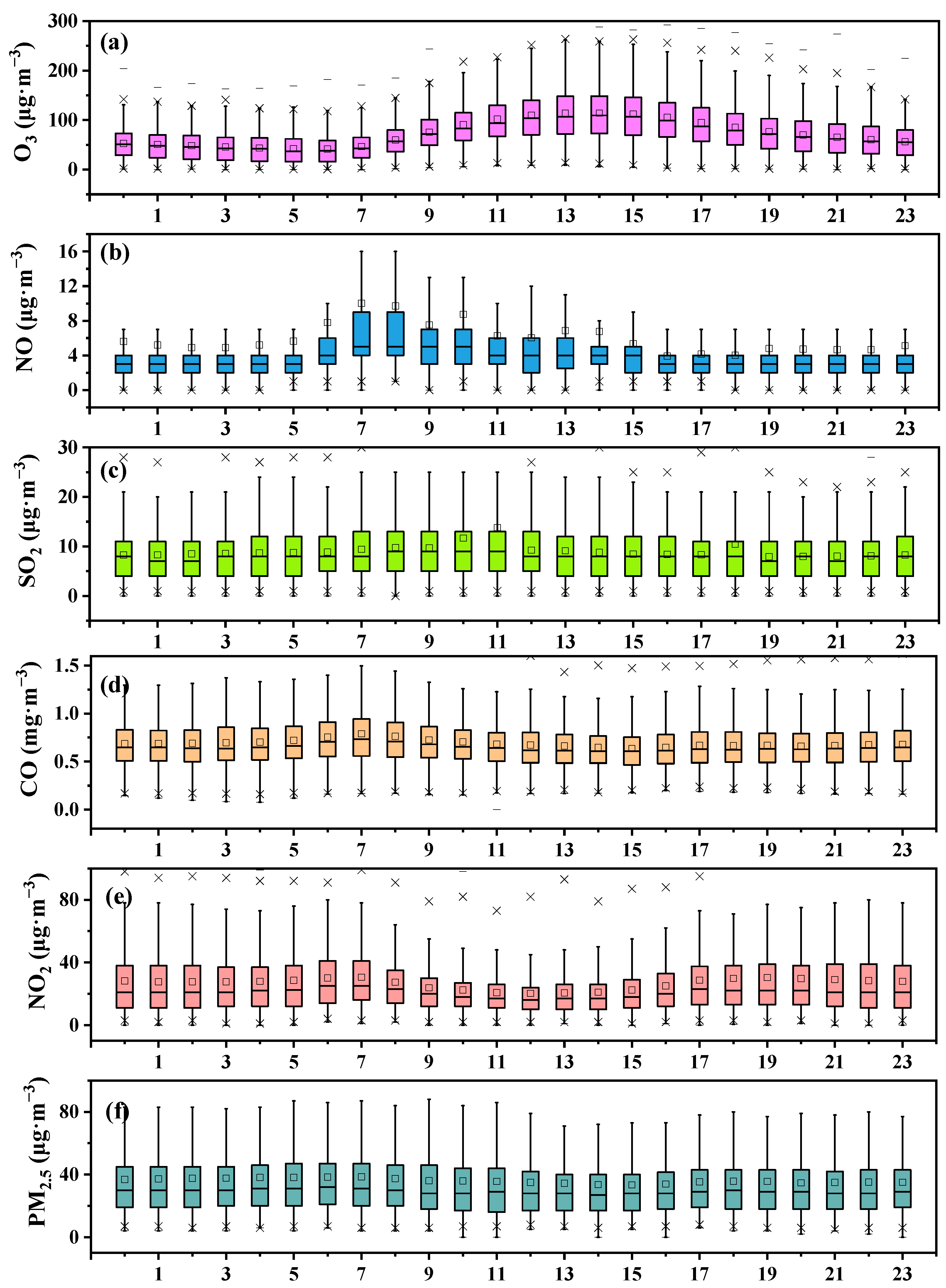
Furthermore, the average diurnal variations in conventional atmospheric pollutants are depicted in Figure 3. Because of photochemical reactions and the “NO titration effect” [26], the maximum ozone concentration was recorded at 13:00–14:00 in the afternoon, while the minimum ozone concentration was recorded at night, ozone concentration fluctuated more during the day than during the evening. NO₂ showed the opposite change pattern with ozone. The concentrations of NO and NO₂ reached a peak at 7:00–8:00 in the morning, which was mainly affected by mobile source emissions during the morning rush hours. Simultaneously, NO₂ and CO shared similar variation trends, which were opposite those of ozone. However, SO₂ and PM_2.5 were insensitive to diurnal changes, which changed without clear regularity.

3.1.2. VOCs

The variations in concentrations and composition of VOCs makes the ozone formation mechanism more complex, so more work needs to be conducted to investigate the characteristics of VOCs [53].

Temporal variations in VOCs were investigated with four groups, including alkanes, aromatics, halocarbons, alkenes, and ethyne, as shown in Figure 4 and Figure S4. There were no obvious seasonal differences in the proportions of the four groups. Overall, the proportion of alkanes was the highest, followed by halocarbons and aromatics, and alkenes and ethyne were least abundant. The concentrations of VOCs from each group were larger in the first semi-year than in the second semi-year, which may be caused by the industrial production cycle. In addition, average diurnal variations in the level of alkanes and halocarbons were not ordered. The level of aromatics, alkenes, and ethyne varied more regularly within a day and showed a single valley at 13:00–14:00, which was significantly affected by photochemical reactions. In summary, the continuity and regularity of VOC concentrations were worse than those of other conventional pollutants because of the effects of both multiple emissions and photochemical reactions.

3.1.3. Meteorological Parameters

Meteorological parameters can affect ozone concentration via mechanisms related to transport, chemical production and consumption, and deposition. The temporal variations in WS, WD, RH, temperature, and P during 2018 were plotted in Figure S5. The average WS was 2.8 m·s⁻¹ with the dominant WD of east and southeast. In addition, larger WS were concentrated in July and August, while other months mainly exhibited smaller WS of 0–4.5 m·s⁻¹ during this year. Therefore, the pollution in the park was mainly affected by the eastern and southeastern oceans, as well as the western and northwestern areas. In addition, the temperature varied from −4.3 °C to 36.3 °C with an annual mean value of 17.7 °C. temperature higher than 17.7 °C were mostly concentrated in M_4–10. More precisely, the temperature distribution in M_4–10 differs significantly from that of other months. The distribution of P was concentrated around approximately 101.31 kPa throughout the year, with variations from 98.5 kPa to 103.5 kPa. The temporal trend for changes in P was opposite to that of temperature, and high P always coexisted with low temperature. RH fluctuated around 83.41% throughout the year, ranging from 21.8% to 100%.

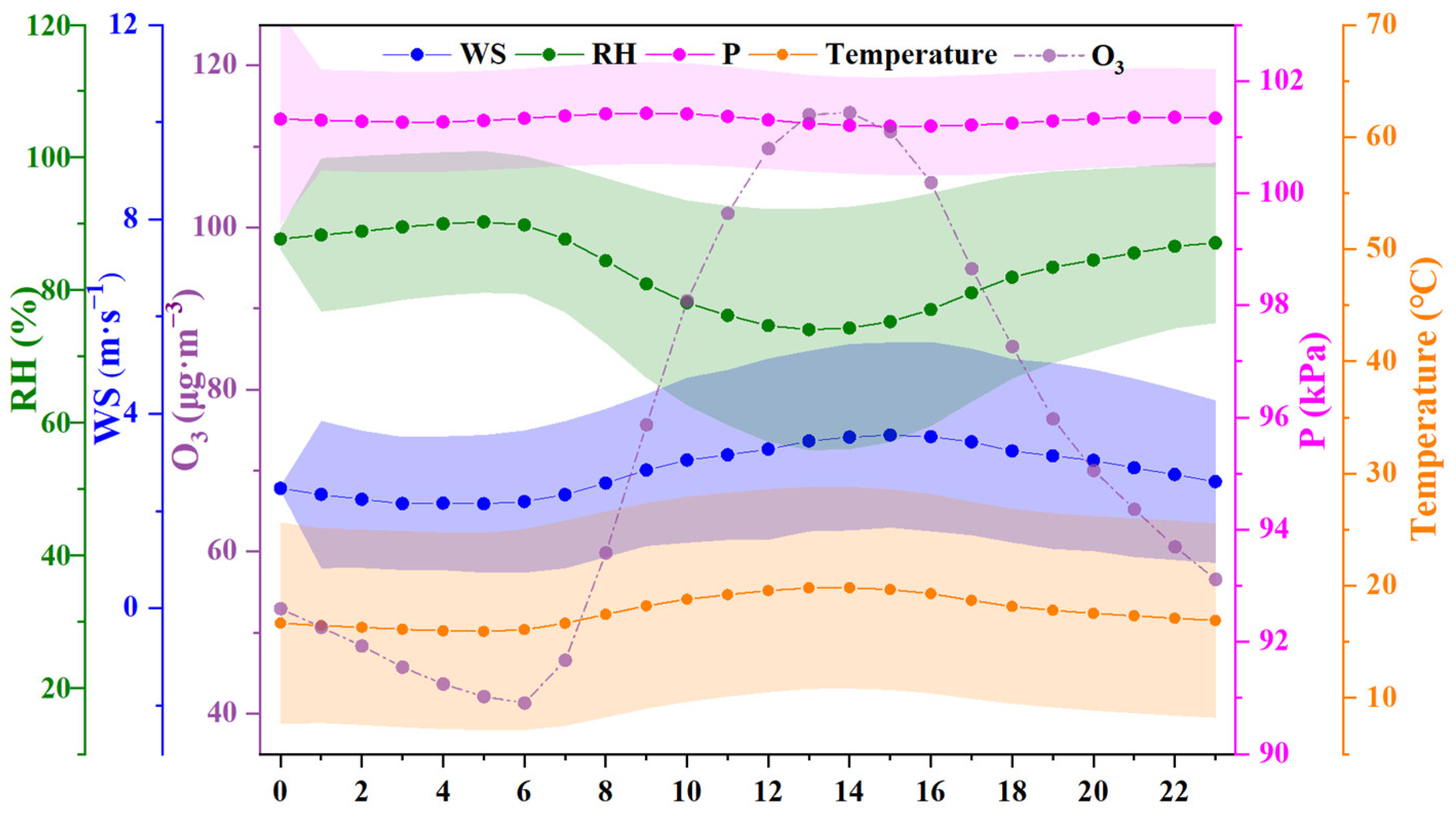
In addition, the average diurnal variations in RH, temperature, WS, and P are also discussed in Figure 5. The diurnal variation curves for temperature, RH, and WS presented single peaks and single valleys. The daily peak for temperature appeared at 13:00, exhibiting consistency with ozone levels but contrasting with those of RH. Coincidentally, WS also showed a similar trend with a valley at 5:00 and a peak at 14:00. Because of the effects of RH, temperature, and atmospheric motion, P showed two peaks at 9:00 and 22:00, with a maximum value at 9:00, and two valleys at 3:00 and 15:00, with a minimum value at 15:00. In addition, the dispersion degrees of temperature, WS and P were stable over time, while that of RH was larger in daytime than at night. Therefore, the relationship between RH and temperature exhibited nonlinearity, potentially impacting their influence on ozone formation.

3.2. Observation-Based Correlation Analysis

Correlation analysis based on observation-based analyses results provide a preliminary understanding of ozone formation rules. Based on the temporal variations in ozone level shown in Figure 3a and Figure S3a, the correlations of impact factors with ozone level were recognized. For conventional atmospheric pollutants, NO₂ and CO exhibited monthly and average diurnal variation trends opposite to those of ozone, as shown in Figure 3d,e and Figure S3d,e. PM_2.5 presented a monthly variation opposite to that of ozone, as shown in Figure S3f. In addition, alkenes and aromatics were separately the VOC groups that exhibited monthly and diurnal changing trends opposite to that of ozone, as shown in Figure 4b,g. The monthly and diurnal variations in ozone levels were consistently influenced by temperature, as depicted in Figure S5a,b and Figure 5. Moreover, elevated temperatures were found to promote the formation of ozone. RH exhibited a trend opposite to that of ozone within a given day (as shown in Figure 5), and high RH inhibited ozone formation. Since reactions among VOCs were more complicated and diverse than those of NO_x, and considering the complex emission conditions and changeable meteorological parameters in the small-scale chemical industrial park, the correlation between O₃ and VOCs was not obvious.

In addition, heavy ozone pollution was mostly concentrated in M_4–10, which accounted for 96.71% of the annual total heavy pollution hours, which was of great significance in exploring the formation rules of ozone pollution in this period.

3.3. Ozone Formation Rules Based on the GBDT Model

3.3.1. Model Performance

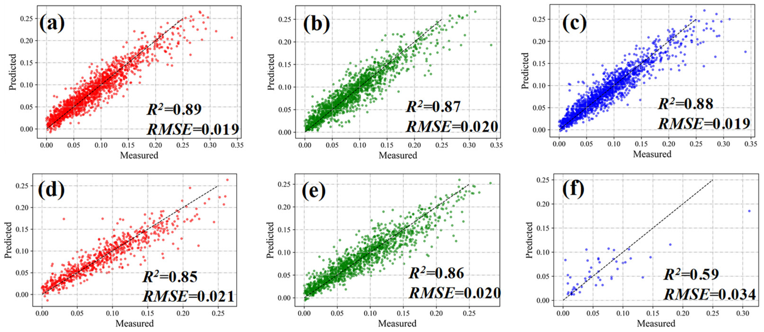
The GBDT model was performed with six input conditions. The best simulation results corresponding to different simulations were shown in Figure 6, which showed that the R² value exceeded 0.85 and RMSE values were less than 0.020 for most simulations, indicating good fits with the GBDT model for ozone concentration in the park. When Comparing different data processing methods, it was observed that the interpolation method outperformed the deletion method in handling missing values. Additionally, the three feature selection methods yielded similar fitting results. Considering these findings collectively, we selected the GBDT model trained using correlation analysis and deletion method for further discussion due to its simplicity and precision.

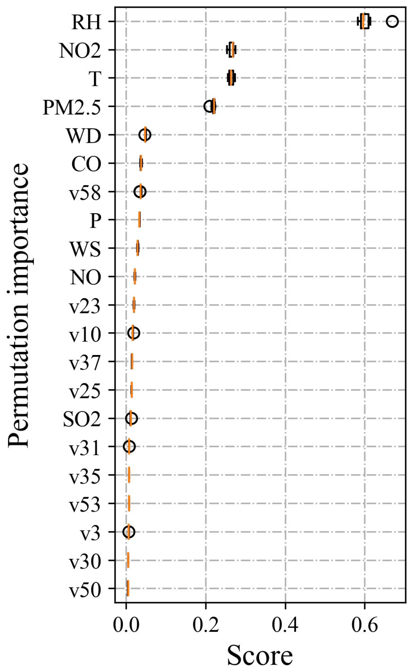
The permutation importance was also used by randomly shuffling the single feature value, which broke the relationship between the features and the target to calculate the decrease in a model score and to confirm the feature importance. After 10 times breaking for the feature order verification, the permutation feature importance results were obtained, as shown in Figure 7. It is obvious that RH, temperature, NO₂, and PM_2.5 were the most important factors determining ozone formation, and the orders of importance for M_4–10 was RH > NO₂ > temperature > PM_2.5. At the same time, the meteorological parameters (mainly RH and temperature) dominated ozone formation. The ozone pollution in the park generally results from the chemical reaction of atmospheric pollutants, which is regulated by meteorological factors. However, it should be noted that the main controlling factors may vary under different conditions.

3.3.2. Ozone Formation Rules

The influencing rules of the dominant factors (RH, temperature, NO₂ and PM_2.5) on ozone formation were further considered to develop a more profound understanding.

(1) 

Meteorological factors (RH and temperature)

Previous results have demonstrated that meteorological factors, particularly RH and temperature, played a dominant role in the formation of ozone pollution in industrial parks. Therefore, this section took a step size of 1% for RH and 0.5 °C for temperature, with a value range of 20–100% for RH and 5–37 °C for temperature to investigate the ozone formation rules using the trained GBDT model. The value of other influencing factors was controlled at their annual mean (prevailing WD) to eliminate their interference.

As shown in Figure 8a, the RH of 50% exhibited the most favorable conditions for ozone accumulation. When the RH was below 50%, variations in RH did not significantly impact ozone formation. When the RH exceeded 50%, there was a decrease in ozone concentration by approximately 1.01 μg·m⁻³ and 2.69 μg·m⁻³ at temperatures ranging from 5 to 20 °C and 25 to 37 °C, respectively, for every increase of 1% RH. The ozone concentration exhibited the highest sensitivity to changes in RH at a temperature of 30 °C. Figure 8b showed that higher temperature led to higher ozone concentrations. Specifically, when the temperature was below 22 °C, ozone concentration exhibited lower sensitivity to temperature at RH exceeding 90%. However, at RH around 80% and within the range of 20–70%, every increase of 1 °C resulted in an elevation of ozone concentration by approximately 1.07 μg·m⁻³ and 1.86 μg·m⁻³, respectively. However, at temperatures above 24 °C, the ozone concentration exhibited an increase of 3.46 μg·m⁻³ and 1.87 μg·m⁻³ for RH of 20–50% and 60–70%, with every increase of 1 °C. A surge in ozone concentration was observed when the temperature increased from 30 °C to 32 °C at an RH of 80–100%. Furthermore, a slight decrease in ozone concentration was observed as the temperature exceeded 35 °C, excessive temperatures were found to inhibit ozone formation. Therefore, high temperatures are conducive to ozone formation and are more likely to result in severe ozone pollution, particularly when the temperature exceeds 30 °C. This finding is consistent with previous studies conducted in this field [26,48].

(2) 

Atmospheric pollutants (NO₂ and PM_2.5)

NO₂ was the main pollutant leading to ozone pollution, and the effect of VOCs should also be considered when exploring the mechanism of NO₂ participation in ozone formation [54,55,56]. The ozone formation mechanism mainly includes two cycles: the NO_x cycle and RO_x (alkoxyl radicals (RO) and organic peroxy radicals (RO₂)) cycle, which are mutually coupled to promote ozone formation [57]. In the atmosphere, NO_x reacts with oxygen radicals and oxygen molecules to provide a closed circulation of ozone through photochemical reactions. At the same time, reactions of HO₂ and RO₂ with NO and the photolysis of NO₂ form the NO_x cycle, which generates ozone without consuming NO_x. The RO_x cycle provides HO₂ and RO₂ persistently to convert NO to NO₂, which also promotes the generation of ozone. Therefore, the ozone concentration is determined by both the concentrations and the ratio of VOCs and NO_x.

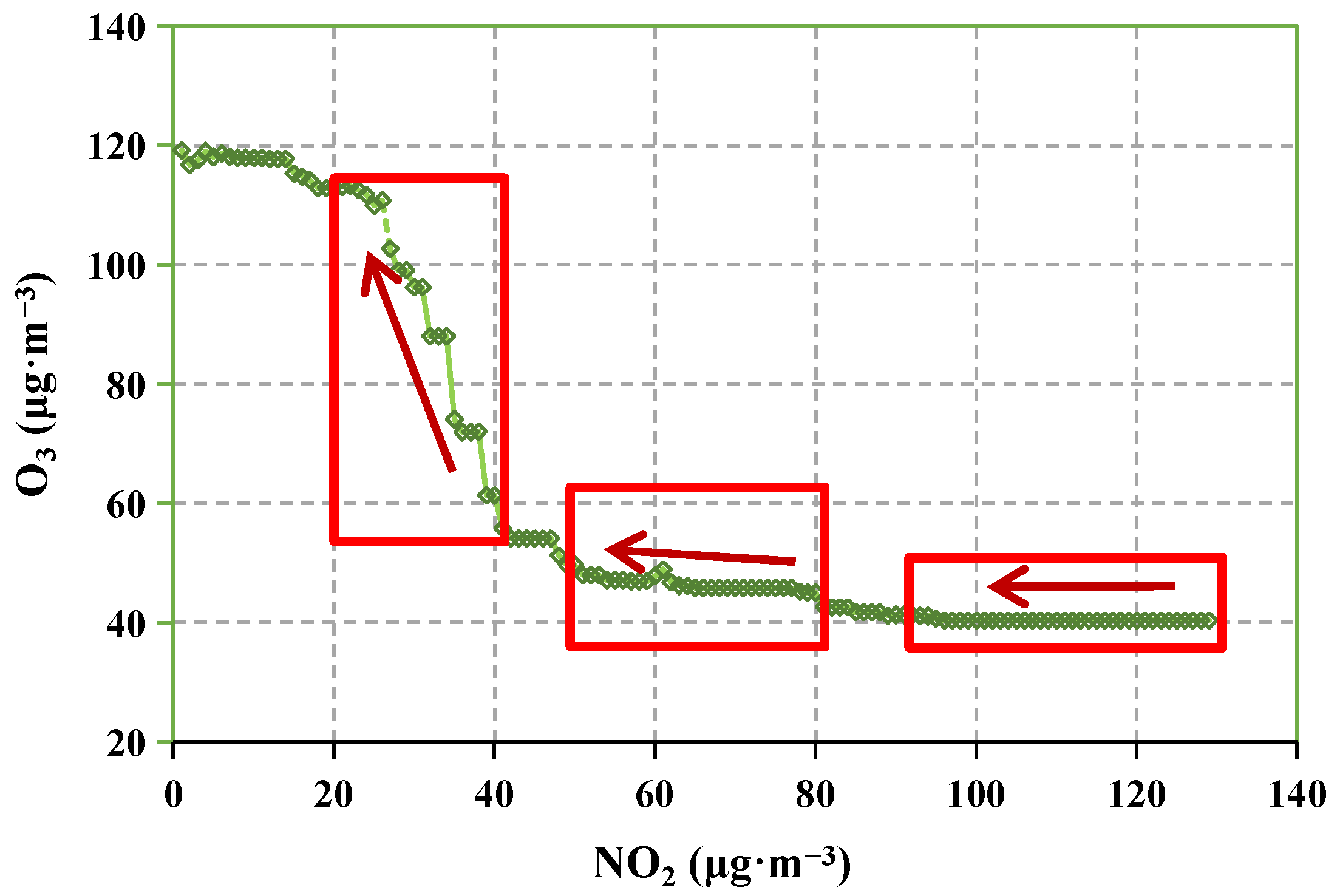
The trained GBDT model was utilized to predict the variation in ozone concentration resulting from 1 μg·m⁻³ increment of NO₂ while keeping other influencing factors controlled at their mean values (prevailing WD). In Figure 9, it was observed that the reduction in NO₂ concentration within the park resulted in an increase in ozone concentration. During the initial phase of declining NO₂ concentration, there was no significant alteration in ozone concentration due to the absence of photochemical reaction at night. Subsequently, during the second phase, a gradual rise in ozone concentration occurred as NO₂ concentration decreased from 80 μg·m⁻³ to 52 μg·m⁻³, with an associated ratio of ozone production to NO₂ consumption equaling 0.10. In the subsequent stage, the ozone concentration exhibited a rapid ascent, while the NO₂ concentration declined from 41 μg·m⁻³ to 20 μg·m⁻³, and the ratio of ozone production to NO₂ consumption reached 2.73. Ultimately, as the NO₂ level diminished, the ozone concentration peaked and subsequently stabilized. Simultaneously, the consumption of ozone during this process resulted in the production of NO₂, exhibiting an essentially contrasting trend.

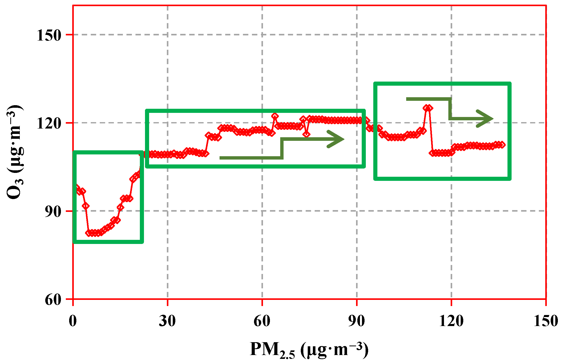
The trained GBDT model was utilized to predict the variation in ozone concentration resulting from a 1 μg·m⁻³ increment in PM_2.5, while maintaining other influencing factors at their mean values (prevailing WD).

As depicted in Figure 10, the relationship between ozone concentration and PM_2.5 concentration exhibited a non-monotonic pattern. When the PM_2.5 concentration was below 25 μg·m⁻³, the relationship followed a V-shaped curve; as the PM_2.5 concentration increased from 25 μg·m⁻³ to 90 μg·m⁻³, the ozone concentration displayed an incremental trend with step-like increases; However, once the PM_2.5 concentration exceeded 90 μg·m⁻³, there was a downward trend in ozone concentration with increasing level of PM_2.5.

4. Discussion

4.1. Ozone Formation Mechanisms

The ozone level of the park was compared with that of stations located without industrial parks within the local city. From 2016 to 2018, the 90th percentile values for maximum daily average 8-h (MDA8) ozone concentrations recorded at the park were 179 μg·m⁻³, 194 μg·m⁻³ and 182 μg·m⁻³, respectively. In contrast, the corresponding concentration at the station located away from the park was found to be lower, with values of 175 μg·m⁻³, 167 μg·m⁻³, and 170 μg·m⁻³ during the same period [58]. Additionally, some other research revealed that industrial parks exhibit distinct local characteristics of VOCs and ozone pollution [22,23,59].

The temporal variation characteristics of pollutants and meteorological parameters revealed that the temporal variation in ozone level exhibited a positive correlation with temperature but an inverse relationship with NO₂, while RH demonstrated stronger correlations compared to other influencing factors. Additionally, the monthly and average daily concentrations of NO₂, CO, and PM_2.5 displayed an opposite trend to that of ozone. The stable meteorological conditions in winter were unfavorable for pollutants dispersion but conducive to the generation of PM_2.5, resulting in high concentrations of NO, NO₂, CO, and PM_2.5. Furthermore, the average daily concentrations variations of ozone, NO₂, NO, and CO were more pronounced than those of other pollutants due to the photochemical reactions, titration effect, and mobile source emissions. Alkenes, ethyne, and aromatics were identified as the unstable factors that impact ozone formation. The differences in the effects of VOCs on ozone were primarily attributed to their varying reactivity. On the one hand, alkenes, ethyne, and aromatics exhibited higher photochemical reactivity compared to other species, thereby exerting stronger influences on ozone formation. On the other hand, alkenes generally displayed faster reaction rates than aromatics, making it more challenging to capture their immediate effects than the cumulative effect, while the opposite situation prevailed for aromatics.

The results of the GBDT model also confirmed the significance of RH, temperature, NO₂, and PM_2.5 in the formation of ozone. One interesting research found that increasing O₃ concentrations during the COVID-19 lockdown and the heavy O₃ pollution event were mainly caused by the photochemistry subject to local air quality and meteorological conditions in petrochemical industrialized Lanzhou city, which was consistent with our research results [60]. Temperature and NO₂ were the key drivers, and RH was the ancillary key driver among all the influencing factors on ambient ozone formation, which was also confirmed in another research [61]. The influencing mechanism of four dominant factors (RH, temperature, NO₂, and PM_2.5) on ozone was comprehensively analyzed in this study.

It was found that ozone pollution in the park was regulated by both RH and temperature. The promotion of ozone concentration growth due to rising temperature was observed to be mitigated by increasing RH, particularly when the RH level reached 90% or higher. The inhibitory effect of high RH clearly counteracted the impact of warming on ozone concentration. The mechanism by which RH influences ozone formation encompasses the following factors. Firstly, an increase in RH leads to a higher likelihood of rainfall, which rapidly reduces ozone concentration through precipitation [26]. Secondly, RH can impact the chemical reaction mechanism involved in ozone formation and consequently induce changes in ozone concentration. Notably, elevated RH level significantly augments the number of hydroxyl radicals available for reacting with and depleting ozone [27,32]. Furthermore, another study has also demonstrated that an elevated RH facilitates the conversion of NO₂ into nitric acid, thereby impeding ozone formation [62]. In our study, temperature exhibited a high sensitivity to ozone, which is consistent with previous research [63]. The influence of temperature on ozone level primarily arises from the following factors. Firstly, elevated temperature induce the thermal decomposition of peroxyacetyl nitrate (PAN), resulting in the generation of ozone precursors and facilitating ozone formation [28,62]. Secondly, increased temperature is often accompanied by heightened radiation and reduced RH, both of which favor ozone formation, as previously discussed. Additionally, higher temperatures promote the natural emission of isoprene [48]. Collectively, these factors contribute to an elevation in concentrations of atmospheric ozone [64].

In this study chemical industrial park, VOCs originate from multiple sources with various reactivity and are emitted through various pathways, leading to fluctuating concentrations and intricate compositions of VOCs within the park, which are relatively oversaturated. Consequently, ozone demonstrates greater sensitivity towards changes in NO_x rather than VOCs. The investigation of industrial regions in Beijing revealed that ozone formation in the industrial site was under a NO_x-limited regime, thereby corroborating the observed sensitivity of ozone to NO₂ in our study [23]. The variation in the ratio between ozone production and NO₂ consumption at different phases is primarily attributed to variations in photochemical reaction rates under diverse meteorological conditions and the concentration of active substances such as VOCs. The insignificant change in ozone concentration under high NO₂ levels can be attributed to two factors. On the one hand, the accumulation of NO₂ is a result of both ozone conversion and emissions from pollution sources. On the other hand, the consumption of NO₂ is primarily influenced by weak photochemical reactions and limited other chemical reactions.

The intricate and dynamic relationship between PM_2.5 and ozone is closely intertwined with their complex changing curve. The impact of PM_2.5 level on ozone formation cannot be simply characterized as promotion or inhibition but rather stems from the intricate web of multiple interactions occurring between them. The heterogeneous chemical processes involving mutual precursors on the surfaces of PM_2.5 exert a significant influence on ozone formation. Furthermore, elevated concentrations of PM_2.5 contribute to increased aerosols optical thickness and reduced photochemical reaction rate [25]. PM can scatter and absorb sunlight, thereby modulating the photolysis rate and subsequently influencing atmospheric oxidation and O₃ generation [65]. Moreover, a decrease in PM concentration leads to a reduction in the total surface area of aerosol as well as the deposition sink of the oxidant, resulting in a deceleration of HO₂ radical deposition on aerosol and subsequent O₃ production [66]. Consequently, it is imperative to integrate measures addressing PM_2.5 levels with those targeting ozone pollution prevention and control to avoid potential trade-offs.

4.2. Control Strategies for Ozone Pollution

The emission of substantial ozone precursors within the park, particularly VOCs and NO_x, gives rise to a distinct scenario wherein ozone pollution exhibits heightened sensitivity to meteorological parameters, notably RH and temperature. Adverse weather conditions can diminish or counteract the efficacy of precursor emissions control measures. Hence, it is imperative to explore their influencing mechanism as previously conducted. Simultaneously, efforts must be made to curtail controllable factors that contribute significantly to ozone formation, especially anthropogenic pollutant emissions.

Firstly, it is crucial to adjust production in accordance with meteorological changes within the park. Implementing seasonal production limitations plays a significant role in preventing and controlling ozone pollution, necessitating comprehensive consideration of enterprises’ production characteristics and capacity utilization based on pollutant discharge license. Secondly, it is imperative to enhance the efficacy of measures aimed at reducing NO_x and active VOC emissions. There is a need to refine the rating scale for air pollution prevention and control within the park while increasing the proportion of petrochemical and chemical enterprises achieving performance ratings of A and B. Additionally, intensified efforts should be directed toward regulating unorganized emissions, with particular emphasis on detecting bypasses in organic waste gas. Enhanced supervision should be implemented for the torch in petrochemical enterprises to minimize the disposal of exhaust gas generated during routine production operations through the torch. Promote the establishment of “fresh parks” and increase the adoption rate of new energy vehicles or those compliant with National-VI emission standards within the park. Finally, during high-temperature periods, it is necessary to implement targeted measures such as reducing the RH of the environment through artificial rainfall and ground sprinkling, as well as reducing precursor emissions through off-peak production. These strategies can effectively regulate peak ozone concentration.

4.3. Advantages, Disadvantages and Prospect

In addition, the advantages and disadvantages of this research were discussed. The data utilized in this study were extracted from a local monitoring station with good integrity. The GBDT model expressed excellent performance in terms of interpretability, accuracy, and robustness in simulating ozone concentration, the same as the outstanding prediction performance discovered in other studies compared to various algorithms such as eXtreme Gradient Boosting (XGBoost), support vector machine (SVM), and multiple linear regression (MLR) in other study [44]. However, aiming to better train the GBDT model, more data with a longer monitoring period, as well as more local monitoring parameters that might be affected by ozone formation, will help, such as meteorology factors of cloud cover and radiation.

Finally, based on our findings, we propose the following suggestions for future research in the relevant areas.

(1)

The investigation of ozone formation rules is conducted through a comprehensive analysis of pollutant emissions from sources and meteorological data using machine learning techniques.

(2)

The assessment of the impacts of dominant factors on ozone levels during days with high ozone pollution compared to those without pollution.

(3)

The exploration of the quantized effects of pollution prevention and control measures on ozone pollution.

5. Conclusions

Ozone and its impact factors, including pollutants (SO₂, NO, NO₂, CO, PM_2.5, and VOCs) and meteorological parameters (RH, temperature, WS, WD, P), were conducted during 2018 to investigate the ozone formation rules in a typical chemical industrial park in the Yangtze River Delta of China. Observation-based analyses and machine learning were used to identify the rules for ozone pollution in the park, which were affected by both the complex emission environment and volatile meteorological parameters. Furthermore, the trained GBDT model was utilized to establish a specific and quantifiable relationship between an individual impact factor and ozone within a complex and uncertain multi-factor context. The research produced the following results, which were helpful for controlling small-scale ozone pollution, improving air quality, and reducing risks to human health.

(1)

The temporal variation of pollutants and meteorological parameters were comprehensively discussed. The ozone level exhibited a temporal variation consistent with temperature but opposite to that of NO₂. RH showed stronger correlations than other influencing factors. Additionally, PM_2.5 and VOCs, particularly alkenes and aromatics, were identified as unstable factors that also influenced ozone formation. Ozone pollution was found to be most prevalent during the months of April to October (M_4–10).

(2)

The GBDT model was employed to investigate the ozone formation rules in M_4–10. Results revealing the importance of permutation revealed that RH, NO₂, temperature, and PM_2.5 were the four most influential factors in ozone formation. The ozone level in the park was found to be more sensitive to meteorological parameters than atmospheric pollutants. An RH of 50% was identified as being most conducive to ozone accumulation. At RH level above 50%, every 1% increase in RH corresponded to a reduction in ozone concentration of approximately 1.01 μg·m⁻³ and 2.69 μg·m⁻³ at temperatures ranging from 5–20 °C and 25–37 °C, respectively. The increase in temperature resulted in elevated ozone concentrations, with the ozone concentration rising by 1.86 μg·m⁻³ and 3.46 μg·m⁻³ at RH levels of 20–50% for temperature ranges of 10–22 °C and 22–36 °C respectively, for every increment of 1 °C. The process of ozone generation resulting from NO₂ depletion can be divided into a steady period, slow climbing period, rapid climbing period, and equilibrium period. The ratio of ozone production to NO₂ consumption was 0.10 and 2.73 as the NO₂ concentration decreased from 80 μg·m⁻³ to 52 μg·m⁻³ and from 41 μg·m⁻³ to 20 μg·m⁻³. Furthermore, the relationship between ozone concentration and PM_2.5 concentration exhibited a non-monotonic pattern.

(3)

The mechanisms of four dominant factors influencing ozone formation were also discussed. Temperature and RH primarily regulate the direction of physical and chemical reactions involved in ozone formation, while NO₂ and PM_2.5 predominantly affect ozone through precursor emissions and chemical reactions. Comprehensive measures need to be implemented for the prevention and control of ozone pollution in industrial parks, including seasonal capacity adjustments and reduction of NO_x and reactive VOC emissions. In future studies, it is essential to enhance the assessment of the impacts exerted by dominant factors on ozone levels during polluted days and non-polluted days while also quantifying the effects of diverse pollution prevention and control measures on ozone concentrations.

References

1. Hsu, C.Y.; Chiang, H.C.; Shie, R.H.; Ku, C.H.; Lin, T.Y.; Chen, M.J.; Chen, N.T.; Chen, Y.C. Ambient VOCs in residential areas near a large-scale petrochemical complex: Spatiotemporal variation, source apportionment and health risk. Environ. Pollut. 2018, 240, 95–104. [Google Scholar] [CrossRef] [PubMed]
2. Huang, Y.; Xiu, G.; Lu, Y.; Gao, S.; Li, L.; Chen, L.; Huang, Q.; Yang, Y.; Che, X.; Chen, X.; et al. Application of an emission profile-based method to trace the sources of volatile organic compounds in a chemical industrial park. Sci. Total Environ. 2021, 768, 144694. [Google Scholar] [CrossRef] [PubMed]
3. Cao, M.Y.; Lin, Y.C.; Zhang, Y.L. Characteristics and Source Apportionment of Atmospheric VOCs in the Nanjing Industrial Area in Autumn. China Environ. Sci. 2020, 41, 2565–2576. [Google Scholar]
4. Cheng, N.N.; Jing, D.J.; Zhang, C.; Chen, Z.W.; Li, W.; Li, S.J.; Wang, Q.L. Process-based VOCs source profiles and contributions to ozone formation and carcinogenic risk in a typical chemical synthesis pharmaceutical industry in China. Sci. Total Environ. 2021, 752, 141899. [Google Scholar] [CrossRef] [PubMed]
5. Wang, Q.L.; Li, S.J.; Dong, M.L.; Li, W.; Gao, X.; Ye, R.M.; Zhang, D.X. VOCs emission characteristics and priority control analysis based on VOCs emission inventories and ozone formation potentials in Zhoushan. Atmos. Environ. 2018, 182, 234–241. [Google Scholar] [CrossRef]
6. Wei, W.; Lv, Z.F.; Li, Y.; Wang, L.T.; Cheng, S.Y.; Liu, H. A WRF-Chem model study of the impact of VOCs emission of a huge petro-chemical industrial zone on the summertime ozone in Beijing, China. Atmos. Environ. 2018, 175, 44–53. [Google Scholar] [CrossRef]
7. Benedict, K.B.; Prenni, A.J.; El-Sayed, M.M.H.; Hecobian, A.; Zhou, Y.; Gebhart, K.A.; Sive, B.C.; Schichtel, B.A.; Collett, J.L. Volatile organic compounds and ozone at four national parks in the southwestern United States. Atmos. Environ. 2020, 239, 117783. [Google Scholar] [CrossRef]
8. Duan, Z.; Yang, Y.; Wang, L.; Liu, C.; Fan, S.; Chen, C.; Tong, Y.; Lin, X.; Gao, Z. Temporal characteristics of carbon dioxide and ozone over a rural-cropland area in the Yangtze River Delta of eastern China. Sci. Total Environ. 2021, 757, 143750. [Google Scholar] [CrossRef] [PubMed]
9. Zeng, J.Y.; Zhang, L.Y.; Yao, C.H.; Xie, T.T.; Rao, L.F.; Lu, H.; Liu, X.C.; Wang, Q.Y.; Lu, S.L. Relationships between chemical elements of PM2.5 and O3 in Shanghai atmosphere based on the 1-year monitoring observation. J. Environ. Sci. 2020, 95, 49–57. [Google Scholar] [CrossRef]
10. Pope, R.J.; Rap, A.; Pimlott, M.A.; Barret, B.; Le Flochmoen, E.; Kerridge, B.J.; Siddans, R.; Latter, B.G.; Ventress, L.J.; Boynard, A.; et al. Quantifying the tropospheric ozone radiative effect and its temporal evolution in the satellite era. Atmos. Chem. Phys. 2024, 24, 3613–3626. [Google Scholar] [CrossRef]
11. Gao, Y.Q.; Li, M.; Wan, X.; Zhao, X.W.; Wu, Y.; Liu, X.X.; Li, X. Important contributions of alkenes and aromatics to VOCs emissions, chemistry and secondary pollutants formation at an industrial site of central eastern China. Atmos. Environ. 2021, 244, 117927. [Google Scholar] [CrossRef]
12. Ou, J.M.; Huang, Z.J.; Klimont, Z.; Jia, G.L.; Zhang, S.H.; Li, C.; Meng, J.; Mi, Z.F.; Zheng, H.R.; Shan, Y.L.; et al. Role of export industries on ozone pollution and its precursors in China. Nat. Commun. 2020, 11, 5492. [Google Scholar] [CrossRef] [PubMed]
13. Xia, S.Y.; Wang, C.; Zhu, B.; Chen, X.; Feng, N.; Yu, G.H.; Huang, X.F. Long-term observations of oxygenated volatile organic compounds (OVOCs) in an urban atmosphere in southern China, 2014–2019. Environ. Pollut. 2021, 270, 116301. [Google Scholar] [CrossRef] [PubMed]
14. Hazarika, S.; Borah, P.; Prakash, A. The assessment of return probability of maximum ozone concentrations in an urban environment of Delhi: A Generalized Extreme Value analysis approach. Atmos. Environ. 2019, 202, 53–63. [Google Scholar] [CrossRef]
15. Lv, D.Q.; Lu, S.H.; Tan, X.; Shao, M.; Xie, S.D.; Wang, L.F. Source profiles, emission factors and associated contributions to secondary pollution of volatile organic compounds (VOCs) emitted from a local petroleum refinery in Shandong. Environ. Pollut. 2021, 274, 116589. [Google Scholar] [CrossRef] [PubMed]
16. Wang, Q.L.; Sheng, D.P.; Wu, C.Z.; Zhao, J.K.; Li, F.L.; Yao, S.D.; Ou, X.J.; Li, W.; Chen, J.M. Exploring ozone formation rules and concentration response to the change of precursors based on artificial neural network simulation in a typical industrial park. Heliyon 2023, 9, e20125. [Google Scholar] [CrossRef] [PubMed]
17. Jing, D.J.; Cheng, N.N.; Zhang, C.; Chen, Z.W.; Cai, X.N.; Li, S.J.; Zhao, J.K.; Wang, Q.L.; Li, W. A novel approach for VOC source apportionment combining characteristic factor and pattern recognition technology in a Chinese industrial area. J. Environ. Sci. 2022, 121, 25–37. [Google Scholar] [CrossRef] [PubMed]
18. Shukla, K.; Dadheech, N.; Kumar, P.; Khare, M. Regression-based flexible models for photochemical air pollutants in the national capital territory of megacity Delhi. Chemosphere 2021, 272, 129611. [Google Scholar] [CrossRef] [PubMed]
19. Swartz, J.S.; Van Zyl, P.G.; Beukes, J.P.; Labuschagne, C.; Brunke, E.G.; Portafaix, T.; Galy-Lacaux, C.; Pienaar, J.J. Twenty-one years of passive sampling monitoring of SO2, NO2 and O3 at the Cape Point GAW station, South Africa. Atmos. Environ. 2020, 222, 117128. [Google Scholar] [CrossRef]
20. Tao, H.R.; Xing, J.; Zhou, H.S.; Pleim, J.; Ran, L.M.; Chang, X.; Wang, S.X.; Chen, F.; Zheng, H.T.; Li, J.H. Impacts of improved modeling resolution on the simulation of meteorology, air quality, and human exposure to PM2.5, O3 in Beijing, China. J. Clean. Prod. 2020, 243, 118574. [Google Scholar] [CrossRef]
21. Liang, C.J.; Cheng, K.L.; Liang, J.J. Quantification of the impact of the offshore petrochemical industrial park on ambient ozone using photochemical grid modeling and assessment monitoring. Environ. Sci. Pollut. Res. 2018, 25, 29752–29765. [Google Scholar] [CrossRef] [PubMed]
22. Lu, Y.; Pang, X.B.; Lyu, Y.; Li, J.J.; Xing, B.; Chen, J.M.; Mao, Y.P.; Shang, Q.Q.; Wu, H.N. Characteristics and sources analysis of ambient volatile organic compounds in a typical industrial park: Implications for ozone formation in 2022 Asian Games. Sci. Total Environ. 2022, 848, 157746. [Google Scholar] [CrossRef] [PubMed]
23. Liu, C.T.; Xin, Y.Y.; Zhang, C.L.; Liu, J.F.; Liu, P.F.; He, X.W.; Mu, Y.J. Ambient volatile organic compounds in urban and industrial regions in Beijing: Characteristics, source apportionment, secondary transformation and health risk assessment. Sci. Total Environ. 2023, 855, 158873. [Google Scholar] [CrossRef] [PubMed]
24. Yao, Y.G.; Yao, S.L.; Wang, D.F. Analysis of a typical ozone pollution event in Suzhou industrial park in spring. Adm. Technol. Environ. Monit. 2023, 35, 26–32. [Google Scholar]
25. Li, J.; Zhai, C.Z.; Yu, J.Y.; Liu, R.L.; Li, Y.Q.; Zeng, L.M.; Xie, S.D. Spatiotemporal variations of ambient volatile organic compounds and their sources in Chongqing, a mountainous megacity in China. Sci. Total Environ. 2018, 627, 1442–1452. [Google Scholar] [CrossRef] [PubMed]
26. Li, Y.S.; Yin, S.S.; Yu, S.J.; Bai, L.; Wang, X.D.; Lu, X.; Ma, S.L. Characteristics of ozone pollution and the sensitivity to precursors during early summer in central plain, China. J. Environ. Sci. 2021, 99, 354–368. [Google Scholar] [CrossRef]
27. Duo, B.; Cui, L.L.; Wang, Z.Z.; Li, R.; Zhang, L.W.; Fu, H.B.; Chen, J.M.; Zhang, H.F.; Qiong, A. Observations of atmospheric pollutants at Lhasa during 2014-2015: Pollution status and the influence of meteorological factors. J. Environ. Sci. 2018, 63, 28–42. [Google Scholar] [CrossRef]
28. Do, K.T. Computational and Geo-Spatial Approaches to Investigate Multi-Scale Air Quality Trends in Southern California. Ph.D. Thesis, University of California, Riverside, CA, USA, 2023. [Google Scholar]
29. Kaffashzadeh, N.; Solmon, F.; Shahbazi, H.; Bidokhti, A.A.A. Trend analysis of measured surface ozone at the megacity of Tehran for the summertime 2007–2021. Atmos. Environ. 2024, 321, 120289. [Google Scholar] [CrossRef]
30. Lee, H.J.; Kuwayama, T.; FitzGibbon, M. Trends of ambient O3 levels associated with O3 precursor gases and meteorology in California: Synergies from ground and satellite observations. Remote Sens. Environ. 2023, 284, 113358. [Google Scholar] [CrossRef]
31. Feng, R.; Wang, Q.; Huang, C.C.; Liang, J.; Luo, K.; Fan, J.R.; Zheng, H.J. Ethylene, xylene, toluene and hexane are major contributors of atmospheric ozone in Hangzhou, China, prior to the 2022 Asian Games. Environ. Chem. Lett. 2019, 17, 1151–1160. [Google Scholar] [CrossRef]
32. Dang, R.J.; Liao, H.; Fu, Y. Quantifying the anthropogenic and meteorological influences on summertime surface ozone in China over 2012–2017. Sci. Total Environ. 2021, 754, 142394. [Google Scholar] [CrossRef] [PubMed]
33. Ge, S.J.; Wang, S.J.; Xu, Q.; Ho, T. Characterization and sensitivity analysis on ozone pollution over the Beaumont-Port Arthur Area in Texas of USA through source apportionment technologies. Atmos. Res. 2021, 247, 105249. [Google Scholar] [CrossRef]
34. Sun, L.; Xue, L.K.; Wang, Y.H.; Li, L.L.; Lin, J.T.; Ni, R.J.; Yan, Y.Y.; Chen, L.L.; Li, J.; Zhang, Q.Z.; et al. Impacts of meteorology and emissions on summertime surface ozone increases over central eastern China between 2003 and 2015. Atmos. Chem. Phys. 2019, 19, 1455–1469. [Google Scholar] [CrossRef]
35. Zhan, Y.; Luo, Y.Z.; Deng, X.F.; Grieneisen, M.L.; Zhang, M.H.; Di, B.F. Spatiotemporal prediction of daily ambient ozone level across China using random forest for human exposure assessment. Environ. Pollut. 2018, 233, 464–473. [Google Scholar] [CrossRef] [PubMed]
36. Huang, K.Y.; Xiao, Q.Y.; Meng, X.; Geng, G.N.; Wang, Y.J.; Lyapustin, A.; Gu, D.F.; Liu, Y. Predicting monthly high-resolution PM2.5 concentrations with random forest model in the North China Plain. Environ. Pollut. 2018, 242, 675–683. [Google Scholar] [CrossRef] [PubMed]
37. Kaminska, J.A. The use of random forests in modelling short-term air pollution effects based on traffic and meteorological conditions: A case study in Wroclaw. J. Environ. Manag. 2018, 217, 164–174. [Google Scholar] [CrossRef] [PubMed]
38. Zhong, H.B.; Zhen, L.; Yao, Q.F.; Xiao, Y.P.; Liu, J.S.; Chen, B.H.; Xu, W. Understanding the spatial and seasonal variation of the ground-level ozone in Southeast China with an interpretable machine learning and multi-source remote sensing. Sci. Total Environ. 2024, 917, 170570. [Google Scholar] [CrossRef] [PubMed]
39. Sayeed, A.; Choi, Y.; Eslami, E.; Lops, Y.; Roy, A.; Jung, J. Using a deep convolutional neural network to predict 2017 ozone concentrations, 24 hours in advance. Neural Netw. 2020, 121, 396–408. [Google Scholar] [CrossRef]
40. Hassan, M.A.; Faheem, M.; Mehmood, T.; Yin, Y.; Liu, J. Assessment of mSeteorological and air quality drivers of elevated ambient ozone in Beijing via machine learning approach. Environ. Sci. Pollut. Res. 2023, 30, 104086–104099. [Google Scholar] [CrossRef] [PubMed]
41. David, M.; Luis, M.A.; Lauret, P. Comparison of intraday probabilistic forecasting of solar irradiance using only endogenous data. Int. J. Forecast. 2018, 34, 529–547. [Google Scholar] [CrossRef]
42. Gu, Q.H.; Chang, Y.X.; Xiong, N.X.; Chen, L. Forecasting Nickel futures price based on the empirical wavelet transform and gradient boosting decision trees. Appl. Soft Comput. 2021, 109, 107472. [Google Scholar] [CrossRef]
43. Zhang, T.N.; He, W.H.; Zheng, H.; Cui, Y.P.; Song, H.Q.; Fu, S.L. Satellite-based ground PM2.5 estimation using a gradient boosting decision tree. Chemosphere 2021, 268, 128801. [Google Scholar] [CrossRef] [PubMed]
44. Luo, Z.Y.; Wang, H.; Li, S.L. Prediction of international roughness index based on stacking fusion model. Sustainability 2022, 14, 6949. [Google Scholar] [CrossRef]
45. Cheng, N.N. Research on Ozone Emission Characteristics, Ozone Influencing Mechanism and Pollution Source Tracing in Typical Chemical Industrial Park. Ph.D. Thesis, Zhejiang University, Hangzhou, China, 2022. [Google Scholar]
46. Jiang, X.Y. Risk Analysis of Chemical Terminal Operation in Zhapu Port Area of Jiaxing Port. Master’s Thesis, Zhejiang Ocean University, Zhoushan, China, 2023. [Google Scholar]
47. Li, Q.Q.; Su, G.J.; Li, C.Q.; Liu, P.F.; Zhao, X.X.; Zhang, C.L.; Sun, X.; Mu, Y.J.; Wu, M.G.; Wang, Q.L.; et al. An investigation into the role of VOCs in SOA and ozone production in Beijing, China. Sci. Total Environ. 2020, 720, 137536. [Google Scholar] [CrossRef] [PubMed]
48. Ma, T.; Duan, F.K.; He, K.B.; Qin, Y.; Tong, D.; Geng, G.N.; Liu, X.Y.; Li, H.; Yang, S.; Ye, S.Q.; et al. Air pollution characteristics and their relationship with emissions and meteorology in the Yangtze River Delta region during 2014–2016. J. Environ. Sci. 2019, 83, 8–20. [Google Scholar] [CrossRef]
49. Xiao, C.C.; Chang, M.; Guo, P.K.; Gu, M.F.; Li, Y. Analysis of air quality characteristics of Beijing-Tianjin-Hebei and its surrounding air pollution transport channel cities in China. J. Environ. Sci. 2020, 87, 213–227. [Google Scholar] [CrossRef] [PubMed]
50. Li, H. Statistical Learning Method, 2nd ed.; Tsinghua University Press: Beijing, China, 2019. [Google Scholar]
51. Stafoggia, M.; Bellander, T.; Bucci, S.; Davoli, M.; Hoogh, K.D.; Donato, F.D.; Gariazzo, C.; Lyapustin, A.; Michelozzi, P.; Renzi, M.; et al. Estimation of daily PM10 and PM2.5 concentrations in Italy, 2013–2015, using a spatiotemporal land-use random-forest model. Environ. Int. 2019, 124, 170–179. [Google Scholar] [CrossRef] [PubMed]
52. Ministry of Ecology and Environmnet of the People’s Republic of China, Ambient air quality standards, 2012.
53. Guan, Y.N.; Wang, L.; Wang, S.J.; Zhang, Y.H.; Xiao, J.Y.; Wang, X.L.; Duan, E.H.; Hou, L.A. Temporal variations and source apportionment of volatile organic compounds at an urban site in Shijiazhuang, China. J. Environ. Sci. 2020, 97, 25–34. [Google Scholar] [CrossRef] [PubMed]
54. Liu, C.Q.; Zhang, L.; Wen, Y.; Shi, K. Sensitivity analysis of O3 formation to its precursors-Multifractal approach. Atmos. Environ. 2021, 251, 118275. [Google Scholar] [CrossRef]
55. Wang, M.; Chen, W.T.; Zhang, L.; Qin, W.; Zhang, Y.; Zhang, X.Z.; Xie, X. Ozone pollution characteristics and sensitivity analysis using an observation-based model in Nanjing, Yangtze River Delta Region of China. J. Environ. Sci. 2020, 93, 13–22. [Google Scholar] [CrossRef] [PubMed]
56. Yang, Y.; Wang, Y.H.; Yao, D.; Zhao, S.M.; Yang, S.H.; Ji, D.S.; Sun, J.; Wang, Y.H.; Liu, Z.R.; Hu, B.; et al. Significant decreases in the volatile organic compound concentration, atmospheric oxidation capacity and photochemical reactivity during the National Day holiday over a suburban site in the North China Plain. Environ. Pollut. 2020, 263, 114657. [Google Scholar] [CrossRef] [PubMed]
57. Lyu, X.P.; Li, K.; Guo, H.; Morawska, L.; Zhou, B.N.; Zeren, Y.Z.; Jiang, F.; Chen, C.H.; Goldstein, A.H.; Xu, X.B.; et al. A synergistic ozone-climate control to address emerging ozone pollution challenges. One Earth 2023, 6, 964–977. [Google Scholar] [CrossRef]
58. Li, L.; Yang, W.D.; Lu, S.; Wu, W.C.; Yuan, J.; Xie, S.Q.; Wu, D.; Li, M.; Cao, M.Y.; Cheng, P. Characteristics of ozone pollution and its relationship with meteorological factors in Jiaxing city. Acta Sci. Nat. Univ. Sunyatseni 2022, 61, 147–153. [Google Scholar]
59. Wang, J.; Yao, Z.; Wang, M.Y.; Chen, S.M.; Long, T.; Wang, H.L.; Li, H.; Guo, X.R.; Hao, J.H.; Nie, L. VOCs Pollution Characteristics and Health Risk Assessment in Typical Industrial Parks in Beijing: Environmental Impact of High and New Technology Industries. Environ. Sci. 2024, 45, 2019–2027. [Google Scholar]
60. Wang, L.; Zhao, Y.; Shi, J.S.; Ma, J.M.; Liu, X.Y.; Han, D.L.; Gao, H.; Huang, T. Predicting ozone formation in petrochemical industrialized Lanzhou city by interpretable ensemble machine learning. Environ. Pollut. 2023, 318, 120798. [Google Scholar] [CrossRef] [PubMed]
61. Xu, H.; Yu, H.F.; Xu, B.; Wang, Z.Y.; Wang, F.; Wei, Y.T.; Liang, W.Q.; Liu, J.X.; Liang, D.N.; Feng, Y.C.; et al. Machine learning coupled structure mining method visualizes the impact of multiple drivers on ambient ozone. Commun. Earth Environ. 2023, 4, 265. [Google Scholar] [CrossRef]
62. Lu, X.; Zhang, L.; Shen, L. Meteorology and climate influences on tropospheric ozone: A review of natural sources, chemistry, and transport patterns. Curr. Pollut. Rep. 2019, 5, 238–260. [Google Scholar] [CrossRef]
63. Rathore, A.; Gopikrishnan, G.S.; Kuttippurath, J. Changes in tropospheric ozone over India: Variability, long-term trends and climate forcing. Atmos. Environ. 2023, 309, 119959. [Google Scholar] [CrossRef]
64. Ma, R.; Ban, J.; Wang, Q.; Zhang, Y.; Yang, Y.; He, M.Z.; Li, S.S.; Shi, W.J.; Li, T.T. Random forest model based fine scale spatiotemporal O3 trends in the Beijing-Tian-Hebei region in China, 2010 to 2017. Environ. Pollut. 2021, 276, 116635. [Google Scholar] [CrossRef] [PubMed]
65. Won, W.S.; Oh, R.; Lee, W.; Ku, S.; Su, P.C.; Yoon, Y.J. Hygroscopic properties of particulate matter and effects of their interactions with weather on visibility. Sci. Rep. 2021, 11, 16401. [Google Scholar] [CrossRef]
66. Ma, S.; Shao, M.; Zhang, Y.; Dai, Q.; Xie, M. Sensitivity of PM2.5 and O3 pollution episodes to meteorological factors over the North China Plain. Sci. Total Environ. 2021, 792, 148474. [Google Scholar] [CrossRef] [PubMed]
Figure 1. The location of the typical chemical industrial park in northeastern Zhejiang Province.
Atmosphere 15 00600 g001
Figure 2. Model operation framework for fitting ozone concentration data.
Atmosphere 15 00600 g002
Figure 3. Average diurnal distributions of O3 (a), SO2 (b), NO (c), NO2 (d), CO (e), and PM2.5 (f) levels in 2018.
Atmosphere 15 00600 g003
Figure 4. Average monthly (ad) and average diurnal (eh) variations in VOCs.
Atmosphere 15 00600 g004
Figure 5. Average diurnal variations in RH, temperature, WS, P, and O3 in 2018 (shaded area: ±SD).
Atmosphere 15 00600 g005
Figure 6. Comparison of the predicted ozone concentration by the GBDT model and measured ozone concentration in M4–10. (Note: (ac) represent the simulation results of interpolation method, while (df) represent the results of deletion method. The red scatter diagram represents the simulation results of correlation analysis method for feature selection, the green scatter diagram represents the simulation results with functional groups method for feature selection, and the blue scatter diagram represents the simulation results without feature selection).
Atmosphere 15 00600 g006
Figure 7. Permutation importance results in M4–10.
Atmosphere 15 00600 g007
Figure 8. Variation curves of RH-O3 at different Temperature (a) and Temperature-O3 at different RH (b).
Atmosphere 15 00600 g008
Figure 9. Variation curve of NO2-O3 in M4–10. (Note: The red squares represent different changing process, the red arrows represent the changing trend, and the green labels represent ozone concentration under varying NO2 level.).
Atmosphere 15 00600 g009
Figure 10. Variation curve of PM2.5-O3 in M4–10. (Note: The green squares represent different changing process, the green arrows represent the changing trend, and the red labels represent ozone concentration under varying PM2.5 level.).
Atmosphere 15 00600 g010