Development of a Refrigerant-Free Cryotrap Unit for Pre-Concentration of Biogenic Volatile Organic Compounds in Air

Abstract

Biogenic volatile organic compounds (BVOCs) are key compounds in atmospheric chemistries, but difficult to measure directly. In this study, a pre-concentration unit combined with gas chromatography-mass spectrometry (GC-MS) was developed for the quantitative analysis of 18 BVOCs in ambient air. The analytes are trapped on an empty silonite-coated tube, which is cooled by a thermoacoustic cooler to cryotrap at −150 °C, and then desorbed by rapid heating to 200 °C. The set-up involves neither the exchange of solid adsorbents nor any further condensation or refocusing steps. Reliable operation is ensured by the thermoacoustic cooler, which neither contains a liquid refrigerant nor requires refilling a cryogen. The pre-concentration unit parameters such as water removal temperature, desorption temperature and desorption time were optimized. All compounds had correlation coefficients that were better than 0.95, and the detection limits were 0.005–0.009 ppbv when the injection volume is 400 mL. The repeatability ranges were 0.9–5.8%. The recoveries were ranged from 81.8% to 93.2%. This new method was applied for the first time to measure ambient BVOCs in suburb Guangzhou in summer 2022. Isoprene concentrations ranged from 0.375 ppbv to 2.98 ppbv. In addition, several extremely low-level monoterpenes (e.g., α-pinene, β-pinene, and D-limonene) were also detected by the method.

1. Introduction

Biogenic volatile organic compounds (BVOCs) include many chemical compounds emitted by plants into the atmosphere, contributing to 75–90% of the total global non-methane VOC emissions in the troposphere [1]. BVOCs play a significant role in influencing the oxidative capacity of the atmosphere at both regional and global scales [2,3]. These compounds react rapidly with the main oxidants, namely hydroxyl (·OH), nitrate (·NO₃) radicals, and ozone (O₃), contributing to the formation of tropospheric O₃ when sufficient nitrogen oxides are present [4,5,6,7,8,9]. O₃ is a greenhouse gas that is harmful to both human health and ecosystems [10,11]. Additionally, BVOCs can form low-volatility compounds and contribute to the creation of secondary organic aerosols (SOA) [12,13,14,15], impacting Earth’s radiative budget [16,17]. Indeed, measurements of ·OH reactivity indicate that a significant fraction of reactive BVOCs in ambient air remain unidentified [18,19]. As such, further instrumental developments to increase the chemical diversity and spatiotemporal resolution of BVOCs observations are fundamental to obtaining a more in-depth understanding of these compounds in atmospheric processes that influence air quality and climate.

Analyzing BVOCs is challenging due to their rapid reactivity and low concentrations, often measured in parts per trillion (ppt). Consequently, a pre-concentration step is essential to detect these compounds effectively. Traditional methods involve collecting BVOCs on solid adsorbents such as porous organic polymers (e.g., Tenax adsorbent) [20,21,22,23] or carbon-based materials (e.g., Carbotrap adsorbent) [24,25,26,27] for 2–3 h. The analytes are then thermally desorbed into a gas chromatography (GC) instrument and detected using a flame ionization detector (FID) or a mass spectrometer (MS) to quantify individual terpene isomers in the laboratory. However, the resolution of sample analysis may not accurately capture the dynamics of BVOC concentration changes in ambient air. The online sorbent sampling coupled with TD-GC or GC-MS methods are rarely reported [27,28]. Furthermore, the use of solid adsorbents can result in measurement errors and interfere with accurate determination [29,30], potentially also posing a risk of penetration [28].

Ultra-low temperature focusing is a technique for capturing VOCs in ambient air that eliminates the need for solid absorbents, thus reducing the potential for measurement errors. Cryogens such as liquid nitrogen (LN₂) [31] or orgon (LAr) [32] offer a lager cooling capacity to trap BVOCs, but they may not be available in rural or remote areas owing to safety restrictions and supply demand. Compression coolers [33,34] offer less cooling capacity in terms of heat lift than liquid nitrogen. However, coolers operating within the range of 350 W–380 W tend to have high operating costs and require liquid cryogens (CFCs), posing a potential leakage risk. Stirling coolers [35] without refrigerants are small in shape; their lowest cold temperature can reach the temperature of liquid nitrogen, but the lateral forces caused by the reciprocating motion of the drive piston can cause seals to wear out, thereby shortening the overall service life of the machine. Thermoacoustic coolers are a perfect solution that is well suited for maintenance-free remote operation [36,37]. Similar to Stirling coolers, they only require electrical power and do not contain any potentially hazardous working fluids or refrigerants to reach the same temperature as liquid nitrogen, and the absence of any mechanical moving parts in the heaters prevents the losses and associated maintenance of Stirling heaters due to mechanical friction. Thus, they can be considered an energy-saving and environmentally friendly refrigeration method. These advantages make thermoacoustic coolers applicable in many industries, such as power plants [38] and liquefaction of natural gases [39]. We are the first to use thermoacoustic coolers for the cryotrapping of VOCs in ambient air. The design of a cryogen-free pre-concentration unit combined with GC-MS/FID instruments has been demonstrated to be suitable for the online monitoring of VOCs, such as alkanes, alkenes, aromatic hydrocarbons, and halogenated hydrocarbons [40,41,42]. Neither a detailed description nor characterization of the pre-concentration unit has been discussed in previous publications.

In this study, we developed a novel enrichment trap for a pre-concentration unit combined with GC-MS/FID for the determination of 18 BVOCs. We also described a general instrument and discussed the pre-concentration parameters. The analytical figures of merit of method were also determined, including the quantification limits and intermediate precision for the target species. The sample methodology was applied to analyze BVOCs in Guangzhou to demonstrate the versatility and reliability of the set-up parameters.

2. Materials and Methods

2.1. Materials

2.1.1. Standard Gas Preparation

Individual standards of 18 BVOCs (Table S1) were prepared and diluted with methanol to a concentration of approximately 0.2 to 1 μg μL⁻¹ of the stock solutions. Aliquots of 100~800 μL of each stock solution were combined into a new, dry glass volumetric flask. The mixture was then diluted to reach a final concentration of approximately 0.02 μg μL⁻¹ of the working solution. A SS Swagelok tee was connected to a clean canister (15 L, Silco-Can, Restek, Bellefonte, PA, USA) equipped with a dynamic dilution system (Nutech 2202B, Plano, TX, USA). The canister was heated to approximately 80 °C. A precision microliter syringe (Hamilton, Reno, NV, USA) was used to inject 2–40 µL of the BVOC mixture working solution from the septum on the SS Swagelok tee into the canister. Subsequently, 0.2 µL of ultrapure water was added to create a wet standard gas mixture at a relative humidity of 50%. After 5 min, the canister was flushed to a set pressure value (29.4 psi) using high-purity nitrogen at a flow rate of 2000 mL min⁻¹ through the standard dilution port [43,44]. The calculated concentration range for each target compound is about ~0.015–6 ppbv.

To evaluate the analytical system, a mixture of 57 non-methane hydrocarbons and a mixture of oxygenated BVOCs (Linde Electronics and Specialty Gases, Danbury, CT, USA) were used in this work as standards for quantitative comparisons, which included the most representative BVOC-emitting species, i.e., isoprene. The VOCs detected by FID were quantified by the external standard method. The components detected by MS were quantified using four internal standards (bromochloromethane, 1,4-difluorobenzene, chlorobenzene-d5, and 4-bromofluorobenzene) [45]. Calibration curves were plotted for two standard gases in the 0.1–8 ppbv range. The VOC species, detection limits (DL) and average concentrations measured by GC-MD/FID are listed in Table S2.

2.1.2. Sample Pre-Concentration

Figure 1a shows the flow scheme of the gas flow during sampling pre-concentration. The sampling tube was a custom-made 3 m stainless steel silonite-coated tube (1/8 OD) heated to 120 °C [46] for ozone removal purposes. A Teflon filter (0.25 µm pore size, 47 mm OD, Millipore Sigma, Burlington, MA, USA) was fitted on the front of the ambient air sampling tube to prevent the migration of particles. Ambient air was sampled and pumped into the pre-concentration unit at a flow rate of 40 mL min⁻¹ during the second 10-min period of each hour. A six-port stream selection valve (Valve 1; Valco Instruments, Houston, TX, USA) was used to direct ambient air and standard gases into the pre-concentration unit. Air samples were then drawn into two parallel channels using a pump for water removal and VOC enrichment. Each channel was equipped with a water trap (H₂O trap, a stainless steel hollow tube with 1/8 inch OD and 2.1 mm ID), an enrichment trap, and a mass flow controller (MFC). The water trap temperatures for Channels 1 and 2, were set at −60 °C and −20 °C, respectively, using Stirling coolers (Cryo S100, China Stirling, Rizhao, China) capable of reaching a minimum temperature of −100 °C. The CO₂ trap in channel 1 was a glass tube (approximately 164 mm with an inner diameter of 4 mm) filled with ascarite CO₂ adsorbent (sodium hydroxide-coated silica, 20–30 mesh, Sigma, Livonia, MI, USA). The enrichment trap for Channel 1 was a porous layer open tubular (PLOT) stainless steel tube with a 0.5 mm ID and a 30 cm length that was designed to trap C2-C4 hydrocarbons, whereas Channel 2 used an empty stainless steel tube (30 cm, 0.76 mm ID) to trap BVOCs and other VOC species in air samples. The temperatures of the enrichment traps for both channels were set at −150 °C [47], and the details of the enrichment trap are described in the next section. In the injection/GC analysis stage, the downstream pump was turned off, the in-port of Valve 1 was switched to S1, and Valve 2 was switched to position B (Figure 1b). The concentrated VOCs in the enrichment traps were volatilized by thermal desorption at 200 °C and were injected into the GC system by helium carrier gas through the transmission tube into the FID column from valve position 4-5-2-3 in channel 1 and into the MS column from valve position 9-8-11-10 in channel 2. After each injection, the pre-concentration unit was blown back for 8 min to remove the residue from the gas tubes. The process was set as follows: the water management trap and enrichment trap of channel 1 and channel 2 were individually heated to 120 °C for 2 min consecutively. Subsequently, the two water traps were heated to 120 °C for 2 min. At the same time, the nitrogen carrier gas passed through V1, the enrichment trap, the CO₂ trap, the water management trap, V4, and V3 at a flow rate of 180 mL min⁻¹, and was discharged through the pump. After the back-blowing stage, the pre-concentrator returned to the idle state again. The sample analysis cycle time was about 1 h, and full autosampling was performed. Customized control software automatically operates the pre-concentrator, which controls system parameters such as water and enrichment trap temperature by cooling and heating with system states such as pre-concentration and desorption.

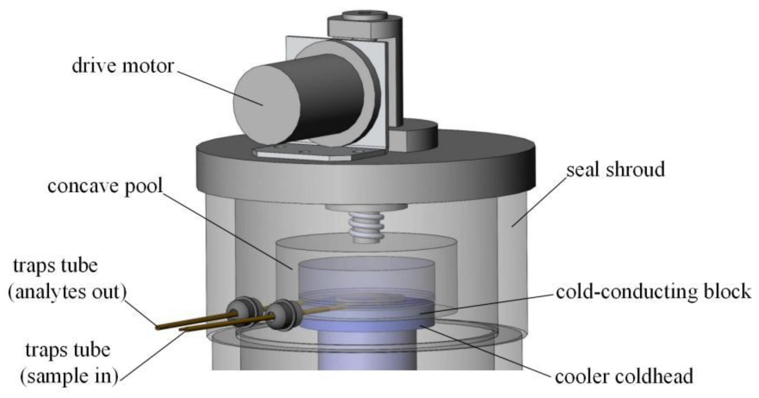
2.1.3. Enrichment Trap and Cooling Technique

Figure 2 shows a technical drawing of the enrichment trap and coldhead. The enrichment trap consists of trapping tubes embedded in a concave pool, which in turn are attached to an insulating sheet, heat-insulating sheet, and aluminum cold-conducting block, which is attached to the cooler coldhead. The coldhead cools the trap tube via cold-conducting block, thus realizing low-temperature VOC trapping. Desorption heating is implemented by pulsing a direct current to the trapping tube. To reduce the heat flowing into the coldhead, in the heating state of the trap tube, we used a drive motor to lift the concave pool of the trap tube away from the coldhead of the cooler and then drop the cold end until the trap tube is heated. The most significant advantage of this structure is that the thermal desorption temperature of the trap tube can reach 260 °C without affecting the normal refrigeration of the cooler, which is conducive to the analysis of low volatile BVOC. Typical cooling and heating cycles are shown in Figure 3 for the sample trap and coldhead. The cooling time from 200 to −150 °C was ~34 min. After the enrichment trap reached its initial set point of −150 °C, the sample trapping cycle began.

Thermoacoustic coolers used for cooling offer the advantage of requiring only electrical power while providing a relatively large cooling capacity at very low minimum temperatures at −196 (77 K), without using cryogens (e.g., liquid nitrogen) and refrigerants (e.g., freon). The cooler should maintain a defined the trapping tubes temperature at −150 °C for VOC enrichment. After thermodesorption, a certain amount of heat flows from the heated trap into the coldhead as the pre-concentration trap is kept directly inside with only a tiny amount of insulation. The excess heat taken by the cooler from the cold header must be released into the surrounding air through the air-fin exhaust heat to quickly reach the cooling state.

2.2. GC-MS/FID Conditions

The traps was rapidly heated to transfer the BVOCs to the GC-MS/FID (7890B GC, 5977B MSD, Agilent Technologies Inc., Santa Clara, CA, USA). BVOCs and other compounds were separated on a semi-polar column (DB-624, 60 m × 0.25 mm ID × 1.4 µm, Agilent Technologies Inc., Santa Clara, CA, USA) and quantified using a quadrupole MS detector. C2–C4 hydrocarbons were separated on a PLOT-AL₂O₃ column (15 m × 0.32 mm ID × 3 μm, Agilent Technologies Inc., Santa Clara, CA, USA) and measured using the FID channel. The GC was programed as follows: 35 °C for 3 min, then increased to 150 °C at a rate of 5 °C min⁻¹, then at a rate of 10 °C min⁻¹ up to 250 °C and maintained for 7 min; and carrier gas (He, 99.999%). The MS detector settings were ionization mode-EI (70 eV), ion source temperature (230 °C), MSD transfer line temperature (240 °C), and total ion chromatogram mass window (40–300 m/z). Retention times were determined by the direct injection of individual BVOC liquid standards into the GCMS. Ion fragmentation was assessed through full scan mode (SCAN) and the NIST (2014) library, as indicated in

Table 1. List of 18 target compounds for ambient measurement, evaporation and freezing points, and quantifier m/z and qualifier m/z values in SIM mode.

Compounds	Evaporation Point (°C)	Freezing Point (°C)	Retention Time (min)	Quantifier m/z	Qualifier m/z
Isoprene	34.1	−146.0	8.8	67	68
α-Pinene	156.1	−62.5	26.1	93	91
Camphene	159.5	52.0	26.9	93	121
Sabinene	163.7	-	27.6	93	91
β-Myrcene	167.0	−10.0	27.8	93	69
β-Pinene	166.0	−61.0	27.8	93	69
2-Carene	167.5	25.0	28.4	93	121, 138
3-Carene	170.2	25.0	28.7	93	91, 79
D-limonene	176.5	−74.0	29.3	93	93, 67
p-Cymene	177.1	−67.9	29.4	119	134, 91
Ocimene	184.1	−27.0	29.6	93	91, 79
Cineole	176.4	1.50	29.7	81	108, 71
γ-Terpinene	182.0	−59.0	30.1	93	91, 136
Isolongifolene	256.0	-	37.7	161	105, 91
Longifolene	257.8	-	38.1	161	94, 91
α-Cedrene	262.0	-	38.1	119	93, 105
β-Caryophyllene	264.0	<25.0	38.2	93	133, 91
α-Caryophyllene	268.0	<25.0	38.9	93	80, 121

- No data.

. Qualitative and quantitative measurements of BVOCs and other compounds in the air samples were carried out simultaneously using SCAN mode and selected ion scan (SIM) mode. The chromatographic separation process took approximately 43 min.

3. Results and Discussion

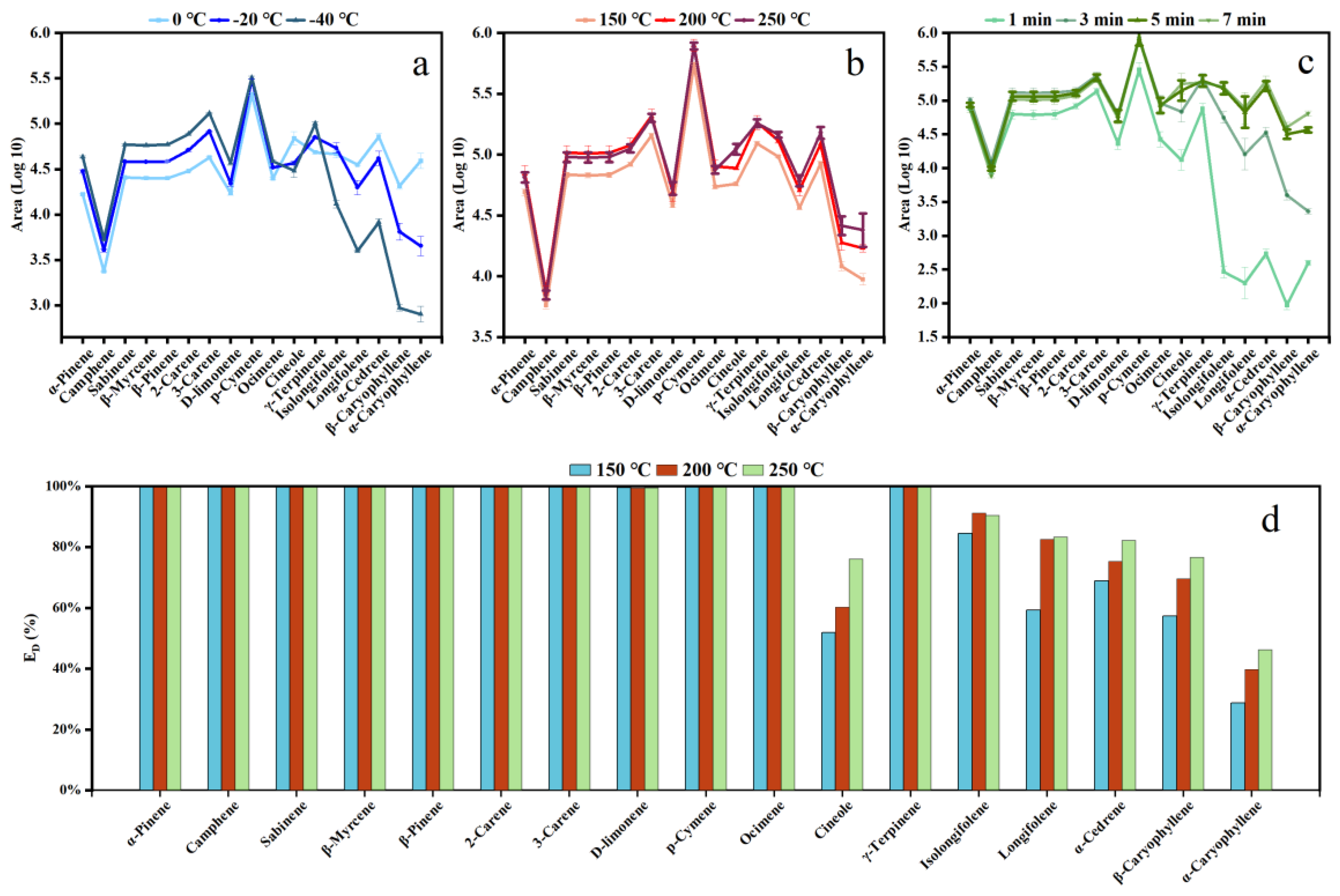
3.1. Optimization of Pre-Concentration Unit Conditions

Different conditions were evaluated to increase BVOC enrichment efficiency. All these conditions were tested at a sample volume of 400 mL, and a mixture of approximately 3–5 ppbv of each BVOC was generated at 50% RH using the dilution system described in the Experimental section. The trap temperature was set at −150 °C, which effectively removed atmospheric moisture during sampling to prevent ice blockage in the trap. During gas chromatography analysis, the water trap was further purged with 180 mL min⁻¹ of dry nitrogen gas for 2 min and heated to 120 °C to reduce the adsorption of the target compounds in the CO₂ and water traps. We tested three different temperatures: 0 °C, −20 °C, and −40 °C. The desorption temperature was set to 200 °C. As shown in Figure 4a, the peak areas of monoterpenes increased with decreasing temperature, while the peak areas of sesquiterpenes decreased with decreasing temperature. The peak areas of cineole decreased slightly, which was caused by the variation in molecular weight and boiling point of the target compounds. Generally, the most volatile compound will be the first to break through the water trap; the larger the molecular weight, the more likely it is to lose a part in the water trap. To reduce the interception of sesquiterpenes and cineole, −20 °C was chosen as the water temperature for this experiment.

The desorption temperature was tested at 150, 200, and 250 °C. For each experiment, a mixture of approximately 3–5 ppbv of each BVOC was generated at 50% RH and sampled using the instrument. Desorption was performed twice at the same temperature. The first chromatogram was obtained from standard gas collection, followed by enrichment traps before GC analysis. Subsequently, without additional operations such as back-flushing or sampling, the trap tubes were directly heated to analyze the targets and generated a second chromatogram. Three replicates were performed for each temperature. Three replicates were performed at each temperature. The desorption efficiency was evaluated at each temperature from Equation (1):

$$E_D\left(\%\right)=\frac{{A_{first}}_i}{{A_{first}}_i+{A_{second}}_i}\times 100$$

(1)

where E_D (%) denotes the desorption efficiency. ${A_{first}}_i$ is the peak area of compound i from the first chromatogram, and ${A_{second}}_i$ is the peak area of compound i from the second chromatogram. Figure 4b shows the peak areas observed for each compound after the first desorption. The desorption efficiency of each compound at various temperatures is shown in Figure 4d. The response increased as the desorption temperature increased, with the monoterpenes peaking at 200 °C and remaining stable at higher temperatures. In contrast, sesquiterpenes and cineole reached peak responses at 250 °C. The response of sesquiterpenes increased by approximately 10%, 16%, 22%, 28%, 29%, and 30% (isolongifolene, longifolene, α-cedrene, β-caryophyllene, α-caryophyllene) from 200 to 250 °C. These results may be attributed to the differences in the molecular weight and the boiling point of the individual compounds. Compared to sesquiterpenes, monoterpenes have lower molecular weight and boiling points; therefore, they were desorbed at lower temperatures. Based on these results, a temperature of 200 °C was considered effective, provided there was sufficient cooling time at the coldhead of the traps.

After the water trap temperature was selected, the desorption time of the trap tubes was optimized from 1 min to 7 min, achieving the highest responses at 200 °C. The results reported in Figure 4c indicate that monoterpenes reached the highest efficiency at 3 min, whereas sesquiterpenes reached the highest efficiency at 5 min, mainly because the boiling point of sesquiterpenes is higher than that of monoterpenes, and the resolution time was longer. To ensure a high efficiency, the desorption time was set to 5 min. Detailed optimization results for target analytes are presented in Table S3 in the Supplementary Materials.

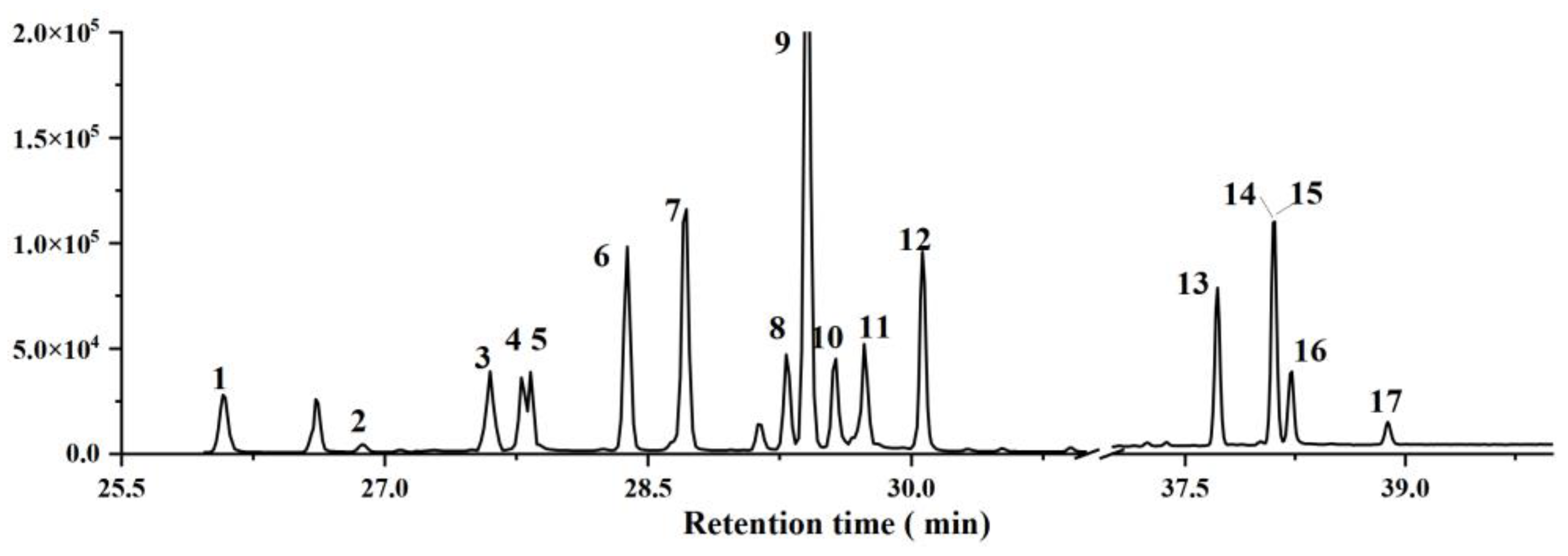
3.2. Overall Performance

To evaluate the overall performance of the optimized method, a mixture of 17 BVOCs was analyzed using a pre-concentrator combined with GC-MS. Isoprene was included in the PAMS mixed standard gas; the chromatographic peak of isoprene and other 17 BVOCs were not in the same chromatogram. Their performances are listed in Table S2. A total of 17 BVOC peaks were separated, as depicted in Figure 5, except for the peaks of myrcene and β-pinene, which belong to the hump described in a previous report [28]. Furthermore, the peaks of longifolene and α-cedrene were co-eluted at 18.1 min Fortunately, the MS quantification ion fragment of longifolene was 161, while that of α-cedrene was 119, allowing for the quantification of these two components based on different fragments. Thus, MS is the best choice for complex isomers and the qualitative quantification of co-eluted peaks. It should be noted that more attention should be paid to the qualitative quantification of these components in complex environmental samples.

Calibration curves were constructed for each BVOC in the concentration range 0.020~2.75 ppbv. The R² values from the scatter plot of the instrument response versus the compound concentration were higher than 0.95 for all of the compounds (

Table 2. The internal standard used for each compound, linear range, calibration equation, linearity (R²), detection limits (DL), repeatablity, recovery, and memory effect.

Order	Compound	Internal Standard	Linear Range (ppbv)	Calibration Equation	R2	DL (ppbv)	Repeatability	Recovery	Memory Effect
1	α-Pinene	IS-3 a	0.022~2.63	y = 14766x − 2005	0.989	0.006	3.8%	85.2%	0.1%
2	Camphene	IS-4 b	0.022~2.63	y = 1736x − 56	0.999	0.007	2.2%	92.8%	1.6%
3	Sabinene	IS-4	0.022~2.63	y = 20215x − 3487	0.974	0.006	3.5%	88.2%	0.1%
4	β-Myrcene	IS-4	0.022~2.63	y = 20051x − 3509	0.973	0.007	4.0%	89.7%	0.1%
5	β-Pinene	IS-4	0.022~2.63	y = 20194x − 3466	0.974	0.008	3.7%	88.2%	0.1%
6	2-Carene	IS-4	0.022~2.63	y = 25584x − 4126	0.984	0.009	3.0%	91.3%	0.1%
7	3-Carene	IS-4	0.022~2.63	y = 47647x − 7274	0.988	0.007	2.7%	92.8%	0.1%
8	D-limonene	IS-4	0.022~2.63	y = 14587x − 2606	0.977	0.008	5.3%	92.8%	1.0%
9	p-Cymene	IS-4	0.023~2.75	y = 185674x − 23335	0.995	0.006	2.0%	88.6%	0.1%
10	Ocimene	IS-4	0.018~2.10	y = 19435x − 2559	0.983	0.007	2.9%	93.2%	0.1%
11	Cineole	IS-4	0.016~1.85	y = 42588x − 6874	0.999	0.006	0.9%	81.8%	0.1%
12	γ-Terpinene	IS-4	0.022~2.63	y = 39384x − 5649	0.987	0.005	4.9%	86.7%	0.1%
13	Isolongifolene	IS-4	0.018~2.10	y = 39203x -2170	0.998	0.007	2.3%	85.6%	0.8%
14	Longifolene	IS-4	0.015~1.75	y = 20635x − 1156	0.997	0.006	1.6%	85.6%	1.0%
15	α-Cedrene	IS-4	0.015~1.75	y = 51656x − 3322	0.996	0.008	3.2%	84.4%	1.0%
16	β-Caryophyllene	IS-4	0.015~1.75	y = 8529x − 892	0.988	0.007	5.2%	86.1%	0.6%
17	α-Caryophyllene	IS-4	0.017~2.00	y = 6580x − 1005	0.975	0.009	5.8%	86.1%	0.7%

^a Chlorobenzene-d5. ^b 4-Bromofluorobenzene.

). The repeatability and recovery were evaluated from seven replicates using a mixture of 0.5 ppbv of the target compounds at 50% RH, and the results are reported in Table 2. The repeatability was fairly good for all compounds lower than 6% under conditions. The recoveries of cineole and cedrene were 81.8% and 84.4%, respectively. Other compounds ranged from 85.2% to 93.2%. The results meet the requirements of analysis. The memory effect was also evaluated by recording a chromatogram of zero air immediately after the chromatogram of the standard gas (3–5 ppbv). The results are reported in Table 2 and were always lower than 2.0% for all compounds. Detection limits were determined for each compound as 3 times the signal-to-noise ratio value. As presented in Table 2, the DL values ranged from 0.005 to 0.009 ppbv when the sampling volume was 400 mL. These values were comparable to the method detection limits for monoterpenes and sesquiterpenes reported in previous TD-GC-MS studies [48,49].

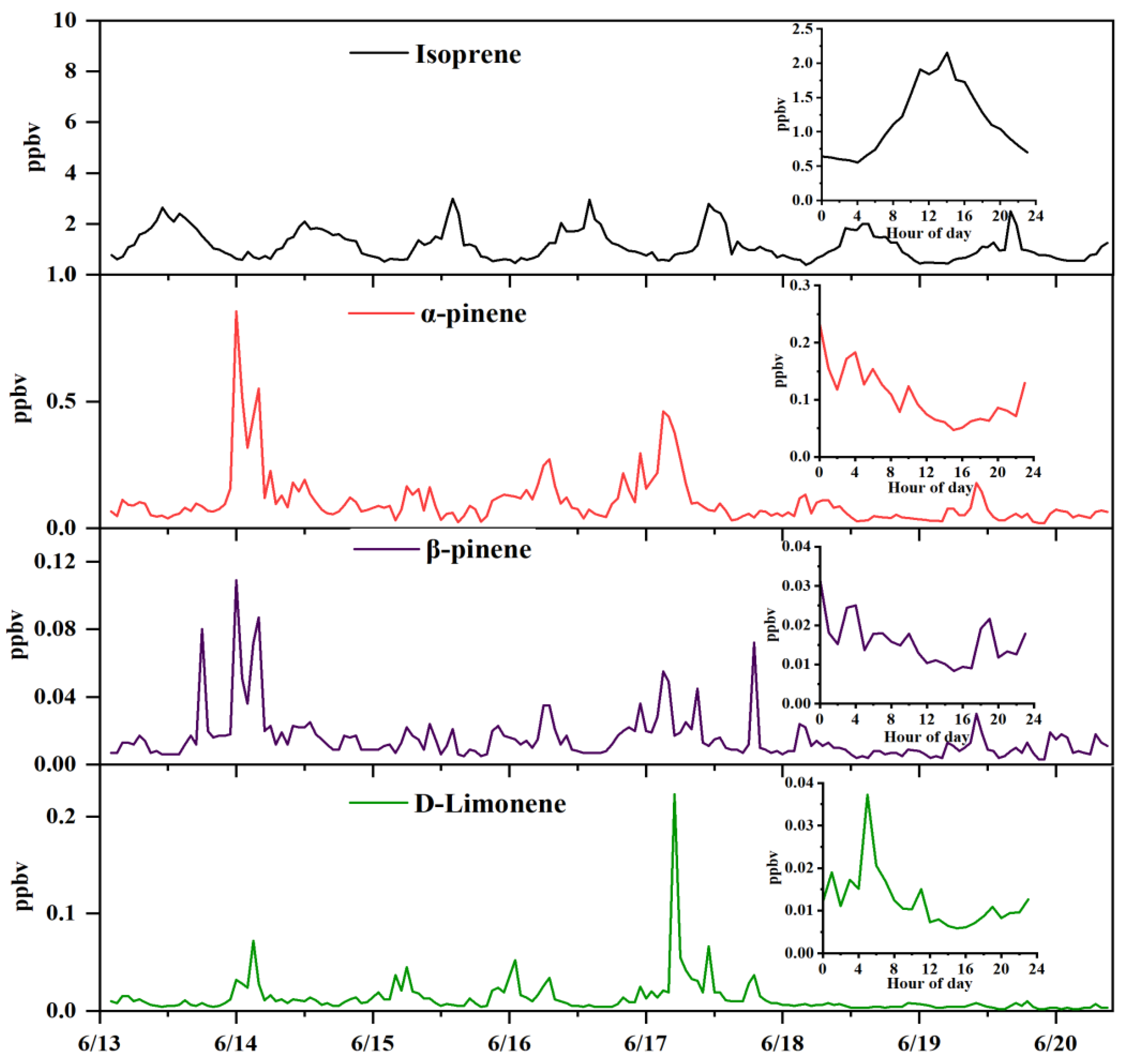
3.3. Real Sample Application

The online cryogen-free GCMS system analyzed BVOCs in ambient air at a site approximately 12 m above the ground on the Laboratory of Institute of Environment and Climate in Jinan University in Guangzhou of China (23°01′ N, 113°24′ E) from 13th to 20th June 2022. Ambient samples were collected at 40 mL min⁻¹ for 10 min, resulting in a total sample volume of 400 mL. The dominant plants on the campus are trees, such as eucalyptus and ficus microcarpa with high isoprene emission potential, and magnolia denudata with high monoterpene emission potential [50]. Figure 6 shows the time series resulting from continuous observations. The average isoprene concentration (1.15 ppbv) was lower than the corresponding values in forest park of Guangzhou in summer [51], and consistent with findings from other locations [32,52,53,54]. The isoprene concentration level was very high during 12:00–16:00, up to 2.98 ppbv, which was consistent with typically diurnal characteristics relating to variations of light and temperature [55,56]. The main monoterpenes were α-Pinene, β-Pinene, and D-limonene. Mixing ratios of α-Pinene ranged from 0.021 to 0.854 ppbv, with a mean concentration of 0.105 ppbv, accounting for 79% of the total monoterpenes. The average concentrations of β-Pinene and D-limonene were 0.016 ppbv and 0.013 ppbv, accounting for 12% and 9% of the total monoterpenes. Table S4 summarizes the average mixing ratios of BVOCs measured in Guangzhou and other sites in China. In general, the monoterpene concentration was lower than that in Guangzhou Forest Park [51], on a mountain in Xi’an [54], or in an urban park in Hong Kong [32]. However, they were higher than those observed using offline canister-sampling measurements in Guangzhou in autumn [52] and in an urban of Beijing [53]. Monoterpenes had the highest concentrations at night (23:00–07:00) and the lowest ones occurred during the daytime, consistent with previously reported results [53,57]. Unlike isoprene, monoterpenes are emitted not only directly by plants’ synthesis under light but also by pool storage. Sesquiterpenes were not detected throughout the monitoring period, which can be explained by the extremely low concentrations in ambient air and the rapid transformation of its higher activity [58,59]. The top ten VOCs measured in this study are presented in Table S5 for comparison with those from cities in China. In general, the average concentrations of the top ten VOCs fell within the ranges reported for other Chinese cities [42,52,60,61,62,63,64]. Levels of iso-pentane and n-pentane, which are important indicators of oil evaporation, were higher than the previous results in a suburb of Guangzhou. This can be explained by the strong intensity of pollution emissions. Through comparison with other studies, it is evident that this method overcomes the limitations of offline sampling in capturing highly reactive and short-lived terpene compounds.

4. Conclusions

A novel cryogen pre-concentration unit was developed and successfully combined with GC-MS/FID to establish and optimize a method for analyzing 18 BVOCs. This method also allows for the simultaneous analysis of other C2-C12 VOCs in the atmosphere with a time resolution of 60 min. The linear ranges of BVOCs were 0.020–2.75 ppbv with linear correlation coefficients (R²) all above 0.95. Detection limits ranged from 0.005 ppbv to 0.009 ppbv with an injection volume of 400 mL, whlie repeatability fell within the range of 0.9–5.8%. The recoveries of BVOCs ranged from 81.8% to 93.2%.

The first measurements using the newly developed method were carried out in the summer of 2022 in Guangzhou. α-Pinene was the most abundant monoterpenes present, with concentrations ranging between 0.021 ppbv and 0.854 ppbv. The 7-day field measurements demonstrated the excellent performance of the methodology with respect to providing speciated BVOC concentration measurements to further investigate atmospheric BVOC reactivity. The set-up has proven to- quantitatively trap and desorb a wide range of trace gases, potentially including hydrocarbons.

The pre-enrichment unit offers several key advantages. Firstly, it eliminates the need for exchanging adsorption tubes, thus removing artifacts associated with the use of solid adsorbents for air sample concentration. Secondly, the split trap structure design allows for a resolution temperature of 200 °C, enhancing the efficiency of resolving BVOC while maintaining the cooler’s normal functionality. Thirdly, the unit utilizes a thermoacoustic cooler to achieve low temperatures, eliminating the need for refrigerant and enabling long-term observations in remote locations. Fourthly, silonite-coated stainless steel or PFA tubes are employed in the sample gas path and centrally heated to minimize wall losses. Additionally, the pre-concentration unit is compact, easy to set up, energy-efficient, and suitable for mobile monitoring. Lastly, the unit can collect BVOC substances with high activity and short lifespans. Overall, the setup is cost-effective, with the thermoacoustic cooler being the most expensive component.

References

1. Sindelarova, K.; Granier, C.; Bouarar, I.; Guenther, A.; Tilmes, S.; Stavrakou, T.; Müller, J.F.; Kuhn, U.; Stefani, P.; Knorr, W. Global data set of biogenic voc emissions calculated by the megan model over the last 30 years. Atmos. Chem. Phys. 2014, 14, 9317–9341. [Google Scholar] [CrossRef]
2. Penuelas, J.; Staudt, M. Bvocs and global change. Trends Plant Sci. 2010, 15, 133–144. [Google Scholar] [CrossRef] [PubMed]
3. Guenther, A. Biological and chemical diversity of biogenic volatile organic emissions into the atmosphere. ISRN Atmos. Sci. 2013, 2013, 1–27. [Google Scholar] [CrossRef]
4. Wolfe, G.M.; Thornton, J.A.; McKay, M.; Goldstein, A.H. Forest-atmosphere exchange of ozone: Sensitivity to very reactive biogenic voc emissions and implications for in-canopy photochemistry. Atmos. Chem. Phys. 2011, 11, 7875–7891. [Google Scholar] [CrossRef]
5. Mo, Z.; Shao, M.; Wang, W.J.; Liu, Y.; Wang, M.; Lu, S.H. Evaluation of biogenic isoprene emissions and their contribution to ozone formation by ground-based measurements in beijing, china. Sci. Total Environ. 2018, 627, 1485–1494. [Google Scholar] [CrossRef]
6. Lou, C.; Jiang, F.; Tian, X.; Zou, Q.; Zheng, Y.; Shen, Y.; Feng, S.; Chen, J.; Zhang, L.; Jia, M.; et al. Modeling the biogenic isoprene emission and its impact on ozone pollution in zhejiang province, china. Sci. Total. Environ 2023, 865, 161212. [Google Scholar] [CrossRef] [PubMed]
7. Sakamoto, Y.; Kohno, N.; Ramasamy, S.; Sato, K.; Morino, Y.; Kajii, Y. Investigation of oh-reactivity budget in the isoprene, α-Pinene and m-xylene oxidation with oh under high nox conditions. Atmos. Environ. 2022, 271, 118916. [Google Scholar] [CrossRef]
8. Li, C.L.; Liu, Y.F.; Cheng, B.F.; Zhang, Y.P.; Liu, X.G.; Qu, Y.; An, J.L.; Kong, L.W. A comprehensive investigation on volatile organic compounds (vocs) in 2018 in beijing, china: Characteristics, sources and behaviours in response to o3 formation. Sci. Total Environ 2022, 806, 150247. [Google Scholar] [CrossRef]
9. Chen, X.; Gong, D.C.; Lin, Y.J.; Xu, Q.; Wang, Y.J.; Liu, S.W.; Li, Q.Q.; Ma, F.Y.; Li, J.Y.; Deng, S.; et al. Emission characteristics of biogenic volatile organic compounds in a subtropical pristine forest of southern china. J. Environ. Sci. 2025, 148, 665–682. [Google Scholar] [CrossRef]
10. Zhao, H.; Zhang, Y.X.; Qi, Q.; Zhang, H.L. Evaluating the impacts of ground-level o3 on crops in china. Curr. Pollut. Rep. 2021, 7, 565–578. [Google Scholar] [CrossRef]
11. Churkina, G.; Kuik, F.; Bonn, B.; Lauer, A.; Grote, R.; Tomiak, K.; Butler, T.M. Effect of voc emissions from vegetation on air quality in berlin during a heatwave. Environ. Sci. Technol. 2017, 51, 6120–6130. [Google Scholar] [CrossRef] [PubMed]
12. Bryant, D.J.; Nelson, B.S.; Swift, S.J.; Budisulistiorini, S.H.; Drysdale, W.S.; Vaughan, A.R.; Newland, M.J.; Hopkins, J.R.; Cash, J.M.; Langford, B.; et al. Biogenic and anthropogenic sources of isoprene and monoterpenes and their secondary organic aerosol in delhi, india. Atmos. Chem. Phys. 2023, 23, 61–83. [Google Scholar] [CrossRef]
13. Ehn, M.; Thornton, J.A.; Kleist, E.; Sipila, M.; Junninen, H.; Pullinen, I.; Springer, M.; Rubach, F.; Tillmann, R.; Lee, B.; et al. A large source of low-volatility secondary organic aerosol. Nature 2014, 506, 476–479. [Google Scholar] [CrossRef]
14. Liu, S.; Xing, J.; Zhang, H.L.; Ding, D.; Zhang, F.F.; Zhao, B.; Sahu, S.K.; Wang, S.X. Climate-driven trends of biogenic volatile organic compound emissions and their impacts on summertime ozone and secondary organic aerosol in china in the 2050s. Atmos. Environ. 2019, 218, 117020. [Google Scholar] [CrossRef]
15. Cao, J.; Situ, S.P.; Hao, Y.F.; Xie, S.D.; Li, L.Y. Enhanced summertime ozone and soa from biogenic volatile organic compound (bvoc) emissions due to vegetation biomass variability during 1981–2018 in china. Atmos. Chem. Phys. 2022, 22, 2351–2364. [Google Scholar] [CrossRef]
16. Chen, T.Y.; Jang, M. Secondary organic aerosol formation from photooxidation of a mixture of dimethyl sulfide and isoprene. Atmos. Environ. 2012, 46, 271–278. [Google Scholar] [CrossRef]
17. Yanez-Serrano, A.M.; Bourtsoukidis, E.; Alves, E.G.; Bauwens, M.; Stavrakou, T.; Llusia, J.; Filella, I.; Guenther, A.; Williams, J.; Artaxo, P.; et al. Amazonian biogenic volatile organic compounds under global change. Glob. Chang. Biol. 2020, 26, 4722–4751. [Google Scholar] [CrossRef]
18. Praplan, A.P.; Tykkä, T.; Schallhart, S.; Tarvainen, V.; Bäck, J.; Hellén, H. Oh reactivity from the emissions of different tree species: Investigating the missing reactivity in a boreal forest. Biogeosciences 2020, 17, 4681–4705. [Google Scholar] [CrossRef]
19. Berndt, T.; Mentler, B.; Scholz, W.; Fischer, L.; Herrmann, H.; Kulmala, M.; Hansel, A. Accretion product formation from ozonolysis and oh radical reaction of alpha-Pinene: Mechanistic insight and the influence of isoprene and ethylene. Environ. Sci.Technol. 2018, 52, 11069–11077. [Google Scholar] [CrossRef] [PubMed]
20. Jones, C.E.; Kato, S.; Nakashima, Y.; Kajii, Y. A novel fast gas chromatography method for higher time resolution measurements of speciated monoterpenes in air. Atmos. Meas. Tech. 2014, 7, 1259–1275. [Google Scholar] [CrossRef]
21. Chen, J.G.; Tang, J.; Yu, X.X. Environmental and physiological controls on diurnal and seasonal patterns of biogenic volatile organic compound emissions from five dominant woody species under field conditions. Environ. Pollut. 2020, 259, 113955. [Google Scholar] [CrossRef] [PubMed]
22. Liu, Y.; Schallhart, S.; Tykkä, T.; Räsänen, M.; Merbold, L.; Hellén, H.; Pellikka, P. Biogenic volatile organic compounds in different ecosystems in southern kenya. Atmos. Environ. 2021, 246, 118064. [Google Scholar] [CrossRef]
23. Tzitzikalaki, E.; Kalivitis, N.; Kouvarakis, G.; Mihalopoulos, N.; Kanakidou, M. Seasonal and diurnal variability of monoterpenes in the eastern mediterranean atmosphere. Atmosphere 2023, 14, 392. [Google Scholar] [CrossRef]
24. Hellén, H.; Schallhart, S.; Praplan, A.P.; Tykkä, T.; Aurela, M.; Lohila, A.; Hakola, H. Sesquiterpenes dominate monoterpenes in northern wetland emissions. Atmos. Chem. Phys. 2020, 20, 7021–7034. [Google Scholar] [CrossRef]
25. Wu, J.; Long, J.Y.; Liu, H.X.; Sun, G.P.; Li, J.; Xu, L.J.; Xu, C.Y. Biogenic volatile organic compounds from 14 landscape woody species: Tree species selection in the construction of urban greenspace with forest healthcare effects. J. Environ. Manag. 2021, 300, 113761. [Google Scholar] [CrossRef]
26. McGlynn, D.F.; Barry, L.E.R.; Lerdau, M.T.; Pusede, S.E.; Isaacman-VanWertz, G. Measurement report: Variability in the composition of biogenic volatile organic compounds in a southeastern us forest and their role in atmospheric reactivity. Atmos. Chem. Phys. 2021, 21, 15755–15770. [Google Scholar] [CrossRef]
27. Helin, A.; Hakola, H.; Hellén, H. Optimisation of a thermal desorption–gas chromatography–mass spectrometry method for the analysis of monoterpenes, sesquiterpenes and diterpenes. Atmos. Meas. Tech. 2020, 13, 3543–3560. [Google Scholar] [CrossRef]
28. Mermet, K.; Sauvage, S.; Dusanter, S.; Salameh, T.; Léonardis, T.; Flaud, P.-M.; Perraudin, É.; Villenave, É.; Locoge, N. Optimization of a gas chromatographic unit for measuring biogenic volatile organic compounds in ambient air. Atmos. Meas. Tech. 2019, 12, 6153–6171. [Google Scholar] [CrossRef]
29. Marcillo, A.; Jakimovska, V.; Widdig, A.; Birkemeyer, C. Comparison of two common adsorption materials for thermal desorption gas chromatography—Mass spectrometry of biogenic volatile organic compounds. J. Chromatogr. A 2017, 1514, 16–28. [Google Scholar] [CrossRef]
30. Lee, J.H.; Batterman, S.A.; Jia, C.; Chernyak, S. Ozone artifacts and carbonyl measurements using tenax gr, tenax ta, carbopack b, and carbopack x adsorbents. J. Air Waste Manag. Assoc. 2006, 56, 1503–1517. [Google Scholar] [CrossRef]
31. Guan, X.; Zhao, Z.; Cai, S.; Wang, S.; Lu, H. Analysis of volatile organic compounds using cryogen-free thermal modulation based comprehensive two-dimensional gas chromatography coupled with quadrupole mass spectrometry. J. Chromatogr. A 2019, 1587, 227–238. [Google Scholar] [CrossRef] [PubMed]
32. Chen, H.W.; Ho, K.-F.; Lee, S.C.; Nichol, J.E. Biogenic volatile organic compounds (bvoc) in ambient air over hong kong: Analytical methodology and field measurement. Int. J. Environ. Anal. Chem. 2010, 90, 988–999. [Google Scholar] [CrossRef]
33. Barkley, C.S.; Zhou, Y.; Troop, D.; Wang, Y.L.; Little, W.C.; Wingenter, O.W.; Russo, R.S.; Varner, R.K.; Talbot, R. Development of a cryogen-free concentration system for measurements of volatile organic compounds. Anal. Chem. 2005, 77, 6989–6998. [Google Scholar]
34. Wang, M.; Zeng, L.M.; Lu, S.H.; Shao, M.; Liu, X.L.; Yu, X.N.; Chen, W.; Yuan, B.; Zhang, Q.; Hu, M.; et al. Development and validation of a cryogen-free automatic gas chromatograph system (gc-ms/fid) for online measurements of volatile organic compounds. Anal. Methods 2014, 6, 9424–9434. [Google Scholar] [CrossRef]
35. Obersteiner, F. A versatile, refrigerant- and cryogen-free cryofocusing–thermodesorption unit for pre-concentration of traces gases in air. Atmos. Meas. Tech. 2016, 9, 5265–5279. [Google Scholar] [CrossRef]
36. Ghorbanian, K.; Karimi, M. Design and optimization of a heat driven thermoacoustic refrigerator. Appl. Therm. Eng. 2014, 62, 653–661. [Google Scholar] [CrossRef]
37. Dai, W.; Luo, E.C.; Hu, J.Y.; Ling, H. A heat-driven thermoacoustic cooler capable of reaching liquid nitrogen temperature. Appl. Phys. Lett. 2005, 86, 224103. [Google Scholar] [CrossRef]
38. Karimi, M.; Ghorbanian, K.; Gholamrezaei, M. Energy and exergy analyses of an integrated gas turbine thermoacoustic engine. Proc. IMechE. Part A J. Power Energy 2011, 225, 389–402. [Google Scholar] [CrossRef]
39. Xu, J.Y.; Luo, E.C.; Hochgreb, S. A thermoacoustic combined cooling, heating, and power (cchp) system for waste heat and lng cold energy recovery. Energy 2021, 227, 120341. [Google Scholar] [CrossRef]
40. Yang, Y.; Ji, D.S.; Sun, J.; Wang, Y.H.; Yao, D.; Zhao, S.M.; Yu, X.N.; Zeng, L.M.; Zhang, R.J.; Zhang, H.; et al. Ambient volatile organic compounds in a suburban site between beijing and tianjin: Concentration levels, source apportionment and health risk assessment. Sci. Total Environ. 2019, 695, 133889. [Google Scholar] [CrossRef]
41. Li, Y.F.; Gao, R.; Xue, L.K.; Wu, Z.H.; Yang, X.; Gao, J.; Ren, L.H.; Li, H.; Ren, Y.Q.; Li, G.; et al. Ambient volatile organic compounds at wudang mountain in central china: Characteristics, sources and implications to ozone formation. Atmos. Res. 2021, 250, 105359. [Google Scholar] [CrossRef]
42. Wu, Y.J.; Fan, X.L.; Liu, Y.; Zhang, J.Q.; Wang, H.; Sun, L.N.; Fang, T.G.; Mao, H.J.; Hu, J.; Wu, L.; et al. Source apportionment of vocs based on photochemical loss in summer at a suburban site in beijing. Atmos. Environ. 2023, 293, 119459. [Google Scholar] [CrossRef]
43. Faiola, C.L.; Erickson, M.H.; Fricaud, V.L.; Jobson, B.T.; VanReken, T.M. Quantification of biogenic volatile organic compounds with a flame ionization detector using the effective carbon number concept. Atmos. Meas. Tech. 2012, 5, 1911–1923. [Google Scholar] [CrossRef]
44. Bouvier-Brown, N.C.; Goldstein, A.H.; Gilman, J.B.; Kuster, W.C.; de Gouw, J.A. In-situ ambient quantification of monoterpenes, sesquiterpenes, and related oxygenated compounds during bearpex 2007: Implications for gas- and particle-phase chemistry. Atmos. Chem. Phys. 2009, 9, 5505–5518. [Google Scholar] [CrossRef]
45. Gong, D.C.; Wang, H.; Zhang, S.Y.; Wang, Y.; Liu, S.C.; Guo, H.; Shao, M.; He, C.R.; Chen, D.H.; He, L.Y.; et al. Low-level summertime isoprene observed at a forested mountaintop site in southern china: Implications for strong regional atmospheric oxidative capacity. Atmos. Chem. Phys. 2018, 18, 14417–14432. [Google Scholar] [CrossRef]
46. Hellén, H.; Kuronen, P.; Hakola, H. Heated stainless steel tube for ozone removal in the ambient air measurements of mono- and sesquiterpenes. Atmos. Environ. 2012, 57, 35–40. [Google Scholar] [CrossRef]
47. Li, H.J.; Xiao, Q.; Han, C.M.; Liu, L.Y.; Fan, X.F.; Chen, N.; Pan, Y.P. On-line monitoring of vocs in ambient air based on cryo-trapping-gc-ms-fid. Environ. Monitoring in China 2017, 33, 101–110. [Google Scholar]
48. Hellén, H.; Praplan, A.P.; Tykkä, T.; Ylivinkka, I.; Vakkari, V.; Bäck, J.; Petäjä, T.; Kulmala, M.; Hakola, H. Long-term measurements of volatile organic compounds highlight the importance of sesquiterpenes for the atmospheric chemistry of a boreal forest. Atmos. Chem. Phys. 2018, 18, 13839–13863. [Google Scholar] [CrossRef]
49. Sheu, R.; Marcotte, A.; Khare, P.; Charan, S.; Ditto, J.C.; Gentner, D.R. Advances in offline approaches for chemically speciated measurements of trace gas-phase organic compounds via adsorbent tubes in an integrated sampling-to-analysis system. J. Chromatogr. A 2018, 1575, 80–90. [Google Scholar] [CrossRef]
50. Zeng, J.q.; Song, W.; Zhang, Y.L.; Mu, Z.b.; Pang, W.H.; Zhang, H.N.; Wang, X.M. Emissions of isoprenoids from dominant tree species in subtropical china. Front. For. Glob. Change 2022, 5, 1089676. [Google Scholar] [CrossRef]
51. Yu, Y.X.; Wen, S.; Lv, H.X.; Wang, X.M.; Sheng, G.; Fu, J.M. Diurnal variations of vocs and relative contribution to ozone in forest of guangzhou. Environ. Sci. Technol. 2009, 32, 94–98. [Google Scholar]
52. Wang, J.; Zhang, Y.L.; Xiao, S.X.; Wu, Z.F.; Wang, X.M. Ozone formation at a suburban site in the pearl river delta region, china: Role of biogenic volatile organic compounds. Atmosphere 2023, 14, 609. [Google Scholar] [CrossRef]
53. Cheng, X.; Li, H.; Zhang, Y.; Li, Y.; Zhang, W.; Wang, X.; Bi, F.; Zhang, H.; Gao, J.; Chai, F.; et al. Atmospheric isoprene and monoterpenes in a typical urban area of beijing: Pollution characterization, chemical reactivity and source identification. J. Environ. Sci. 2018, 71, 150–167. [Google Scholar] [CrossRef] [PubMed]
54. Li, N.; He, Q.Y.; Greenberg, J.; Guenther, A.; Li, J.Y.; Cao, J.J.; Wang, J.; Liao, H.; Wang, Q.Y.; Zhang, Q. Impacts of biogenic and anthropogenic emissions on summertime ozone formation in the guanzhong basin, china. Atmos. Chem. Phys. 2018, 18, 7489–7507. [Google Scholar] [CrossRef]
55. Guo, H.; Ling, Z.H.; Simpson, I.J.; Blake, D.R.; Wang, D.W. Observations of isoprene, methacrolein (mac) and methyl vinyl ketone (mvk) at a mountain site in hong kong. J. Geophys. Res. 2012, 117, D19303. [Google Scholar] [CrossRef]
56. Dos Santos, T.C.; Dominutti, P.; Pedrosa, G.S.; Coelho, M.S.; Nogueira, T.; Borbon, A.; Souza, S.R.; Fornaro, A. Isoprene in urban atlantic forests: Variability, origin, and implications on the air quality of a subtropical megacity. Sci. Total Environ 2022, 824, 153728. [Google Scholar] [CrossRef] [PubMed]
57. Hellén, H.; Tykkä, T.; Hakola, H. Importance of monoterpenes and isoprene in urban air in northern europe. Atmos. Environ. 2012, 59, 59–66. [Google Scholar] [CrossRef]
58. Li, H.Y.; Canagaratna, M.R.; Riva, M.; Rantala, P.; Zhang, Y.J.; Thomas, S.; Heikkinen, L.; Flaud, P.-M.; Villenave, E.; Perraudin, E.; et al. Atmospheric organic vapors in two european pine forests measured by a vocus ptr-tof: Insights into monoterpene and sesquiterpene oxidation processes. Atmos. Chem. Phys. 2021, 21, 4123–4147. [Google Scholar] [CrossRef]
59. Yee, L.D.; Isaacman-VanWertz, G.; Wernis, R.A.; Meng, M.; Rivera, V.; Kreisberg, N.M.; Hering, S.V.; Bering, M.S.; Glasius, M.; Upshur, M.A.; et al. Observations of sesquiterpenes and their oxidation products in central amazonia during the wet and dry seasons. Atmos. Chem. Phys. 2018, 18, 10433–10457. [Google Scholar] [CrossRef]
60. Zou, Y.; Deng, X.J.; Zhu, D.; Gong, D.C.; Wang, H.; Li, F.; Tan, H.B.; Deng, T.; Mai, B.R.; Liu, X.T.; et al. Characteristics of 1 year of observational data of vocs, nox and o3 at a suburban site in guangzhou, china. Atmos. Chem. Phys. 2015, 15, 6625–6636. [Google Scholar] [CrossRef]
61. Yang, W.Q.; Yu, Q.Q.; Pei, C.L.; Liao, C.H.; Liu, J.J.; Zhang, J.P.; Zhang, Y.L.; Qiu, X.N.; Zhang, T.; Zhang, Y.B.; et al. Characteristics of volatile organic compounds in the pearl river delta region, china: Chemical reactivity, source, and emission regions. Atmosphere 2021, 13, 9. [Google Scholar] [CrossRef]
62. Meng, Y.; Song, J.W.; Zeng, L.W.; Zhang, Y.Y.; Zhao, Y.; Liu, X.F.; Guo, H.; Zhong, L.J.; Ou, Y.B.; Zhou, Y.; et al. Ambient volatile organic compounds at a receptor site in the pearl river delta region: Variations, source apportionment and effects on ozone formation. J. Environ. Sci 2022, 111, 104–117. [Google Scholar] [CrossRef] [PubMed]
63. Liu, Y.H.; Wang, H.L.; Jing, S.G.; Gao, Y.Q.; Peng, Y.R.; Lou, S.R.; Cheng, T.T.; Tao, S.K.; Li, L.; Li, Y.J.; et al. Characteristics and sources of volatile organic compounds (vocs) in shanghai during summer: Implications of regional transport. Atmos. Environ. 2019, 215, 116902. [Google Scholar] [CrossRef]
64. Hui, L.R.; Liu, X.G.; Tan, Q.W.; Feng, M.; An, J.L.; Qu, Y.; Zhang, Y.H.; Deng, Y.J.; Zhai, R.X.; Wang, Z. Voc characteristics, chemical reactivity and sources in urban wuhan, central china. Atmos. Environ. 2020, 224, 117340. [Google Scholar] [CrossRef]
Figure 1. Flow scheme showing the gas flow. (a) Position A in Valve 2, sampling pre-concentration sate; (b) Position B in Valve 2, sampling injection state. The green line shows the gas path. S1–S6 denote the positions of Valve 1. The number of Valve 2 denote the Valve positions. V1, V2, V3, V4 denote solenoid valves.
Atmosphere 15 00587 g001
Figure 2. Technical drawing of the coldhead and cryotrap placed inside.
Atmosphere 15 00587 g002
Figure 3. Cooling and heating cycles of the sampling enrichment trap and coldhead of the cooler loops.
Atmosphere 15 00587 g003
Figure 4. Optimization of pre-concentration unit conditions for BVOC measurements. (a) the water trap temperature, (b) the desorption temperature, (c) the desorption time, (d) the desorption efficiency. The error bars represent reproducibility (n = 3).
Atmosphere 15 00587 g004
Figure 5. Separation of BVOCs using a DB-624 column. VOC mixing ratios were approximately 2 ppbv. The peaks in order from left to right were: 1. α-Pinene, 2. Camphene, 3. Sabinene, 4. β-Myrcene, 5. β-Pinene, 6. 2-Carene, 7. 3-Carene, 8. D-limonene, 9. p-Cymene, 10. Ocimene, 11. Cineole, 12. γ-Terpinene, 13. Isolongifolene, 14. Longifolene, 15. α-Cedrene, 16. β-Caryophyllene, 17. α-Caryophyllene.
Atmosphere 15 00587 g005
Figure 6. Time series of concentrations for a selection of the BVOCs observed in Guangzhou.
Atmosphere 15 00587 g006