


Hydrological Drought and Flood Projection in the Upper Heihe River Basin Based on a Multi-GCM Ensemble and the Optimal GCM


Abstract
1. Introduction
2. Study Area and Data Description
2.1. Study Area
2.2. Data Description
3. Study Methods
3.1. SWAT Model and Performance Evaluation
3.2. Data Bias Correction
3.3. Optimal GCM Selection and MME
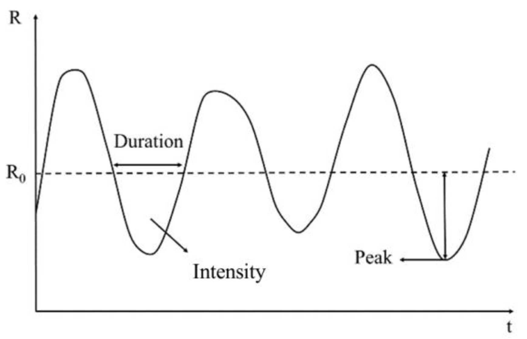
3.4. Standardized Runoff Index and Drought/Flood Characteristic Variables
4. Results and Analysis
4.1. Historical Runoff Simulation and Hydrological Drought and Flood Assessment
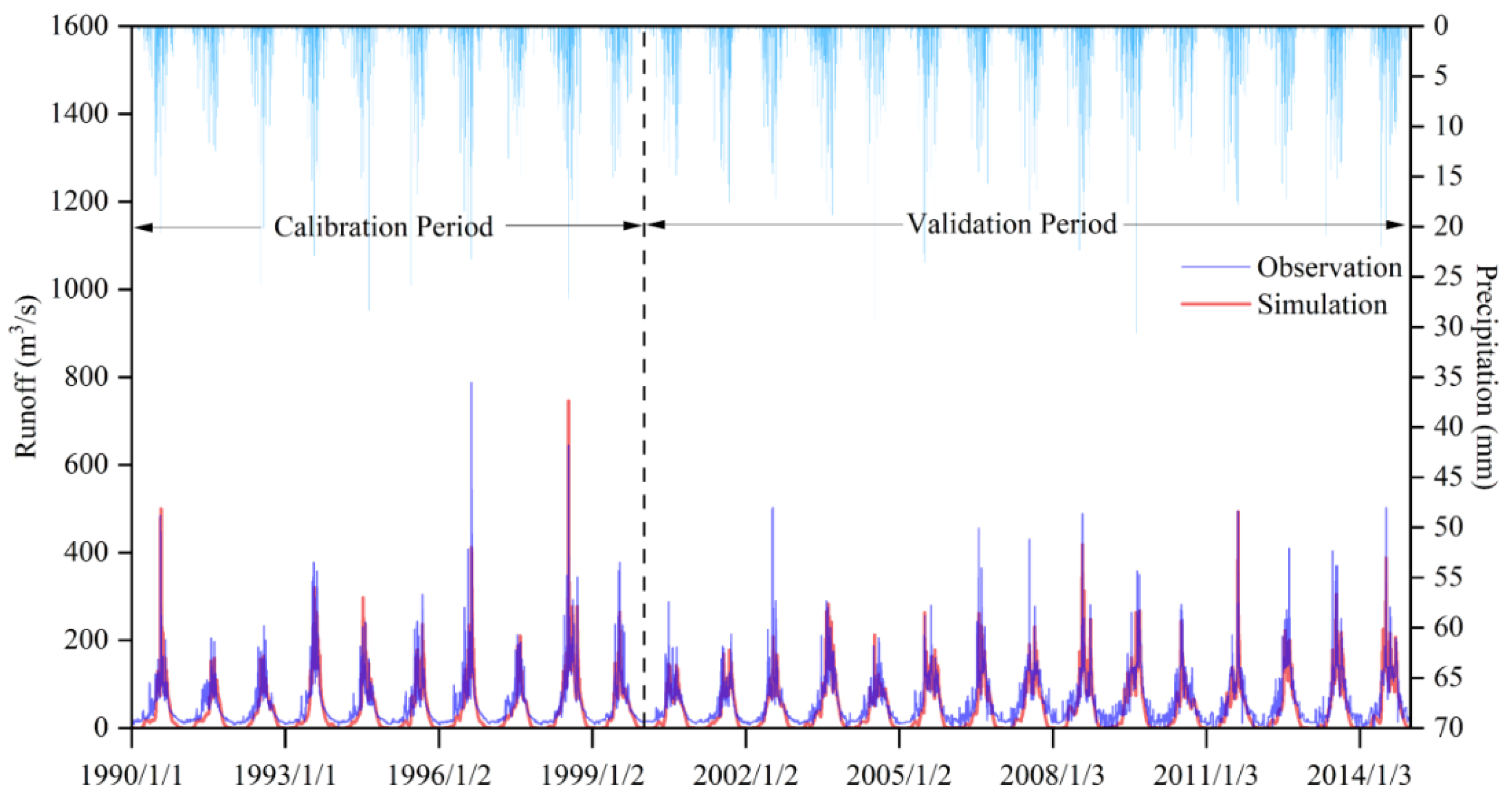
4.1.1. Historical Runoff Simulation
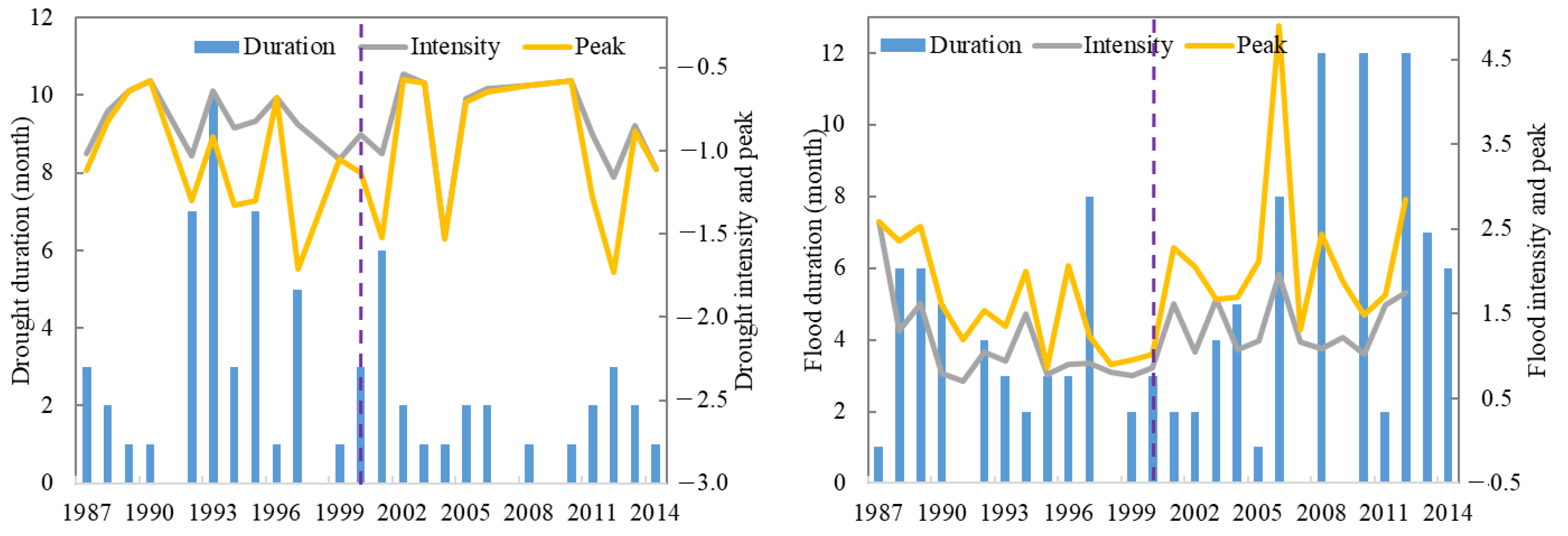
4.1.2. Historical Hydrological Drought and Flood Assessment
4.2. Future Runoff Projection and Analysis
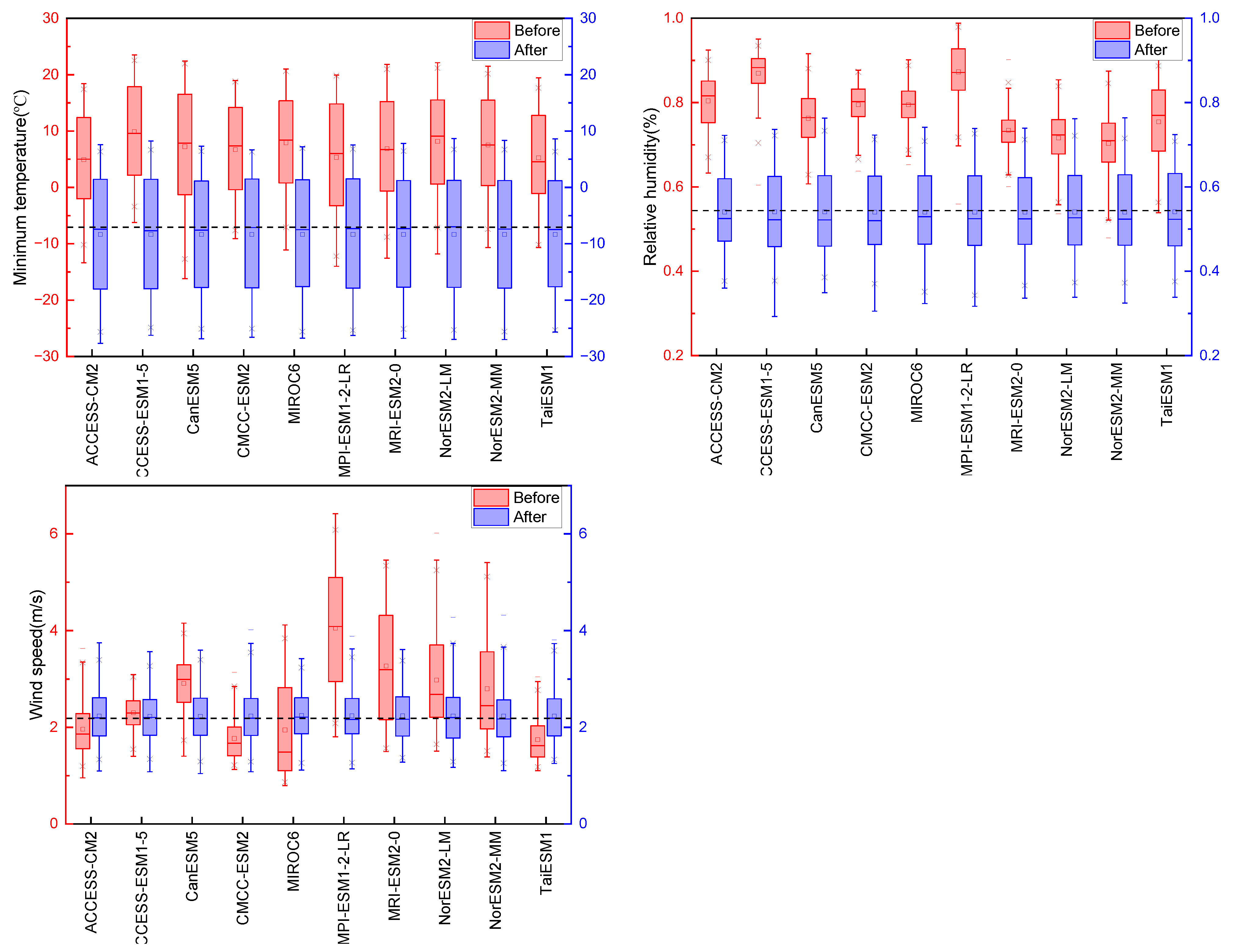
4.2.1. Bias Correction of GCM Output
4.2.2. Optimal GCM Selection
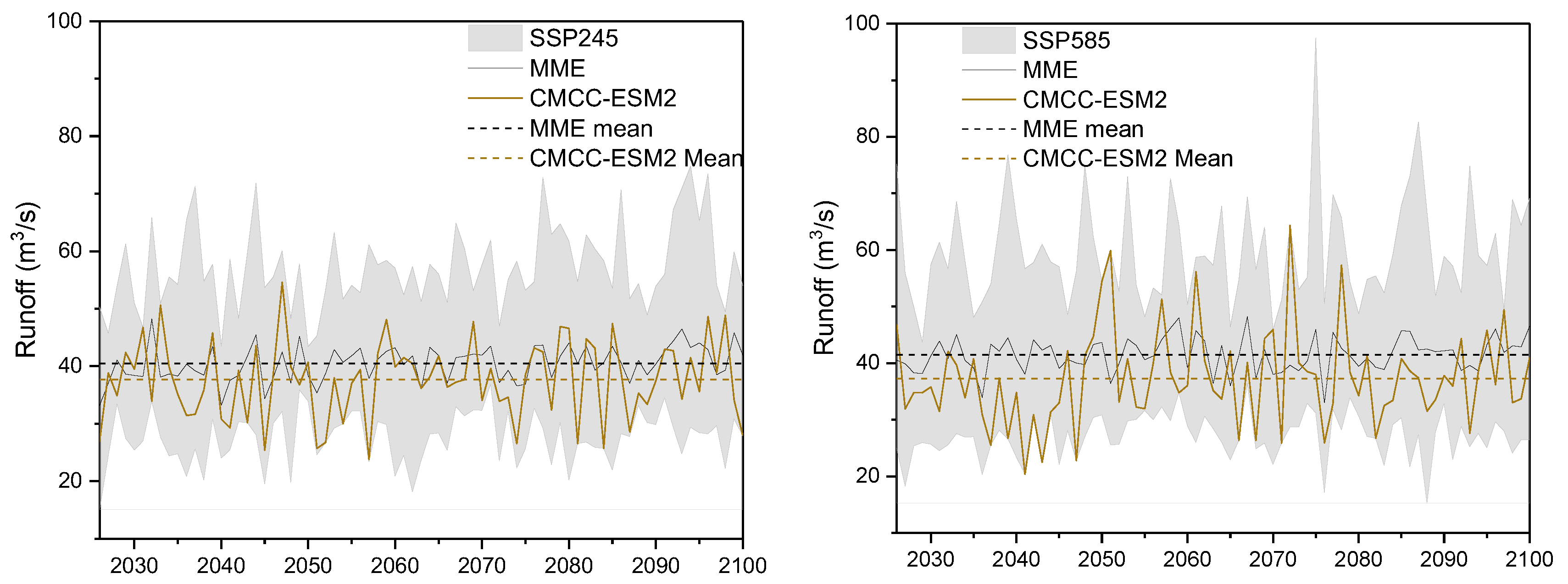
4.2.3. Future Projected Runoff
4.3. Future Hydrological Drought and Flood Projection and Analysis
4.3.1. Hydrological Drought
Drought Duration
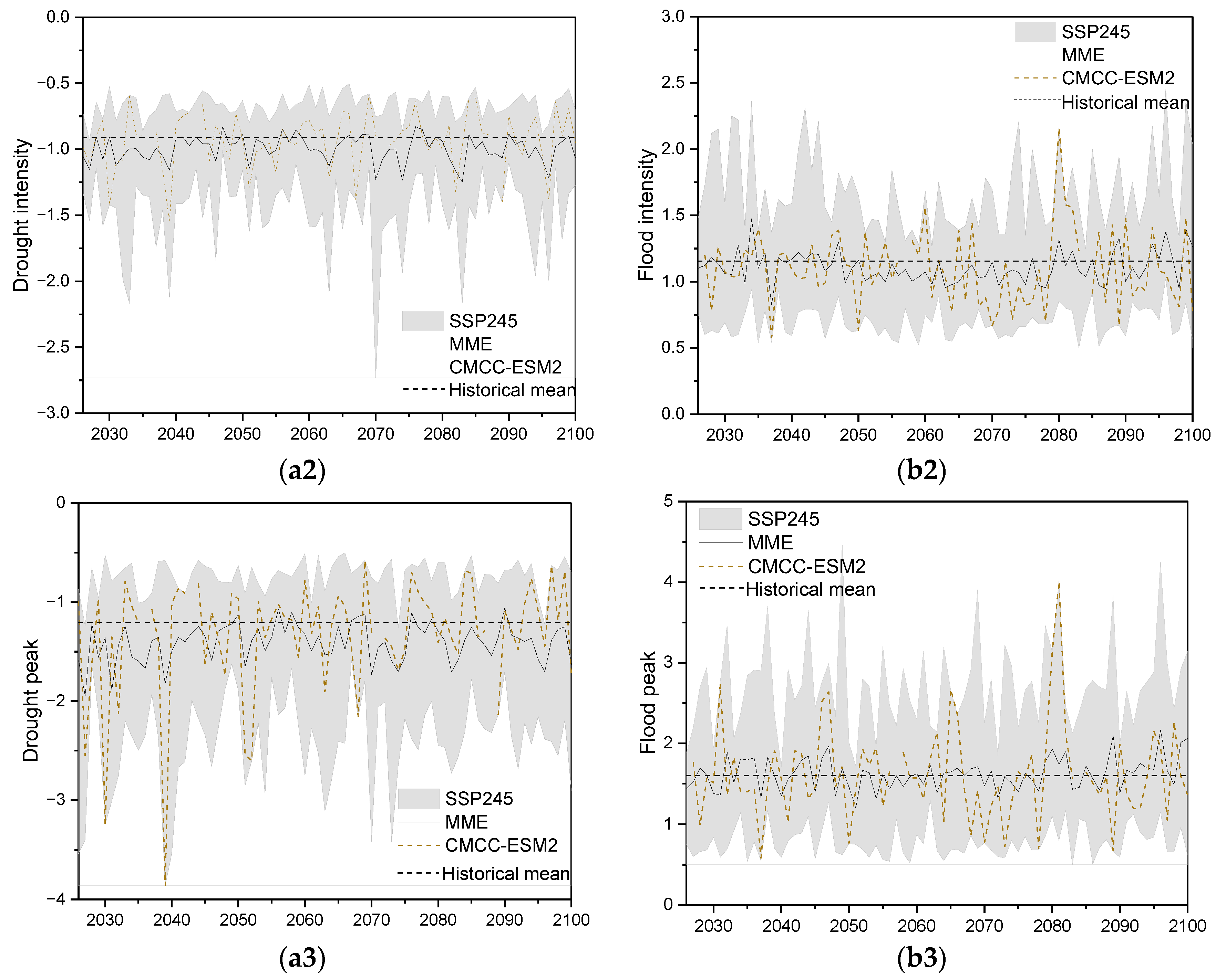
Drought Intensity
Drought Peak
4.3.2. Flood
Flood Duration
Flood Intensity
Flood Peak
4.4. Discussion
4.4.1. Historical Hydrological Drought and Floods
4.4.2. Future Runoff
4.4.3. Future Hydrological Drought and Flood
5. Conclusions
- (1)
- Large differences exist in future runoff projections by different GCMs. The multi-year average runoff projected by the MME was close to the historical period (1987–2014) under the SSP245 scenario, and increased by 2.3% under the SSP585 scenario. The optimal model CMCC-ESM2, which was determined by the entropy-weighted TOPSIS method, projected a decreased runoff in the future, decreasing by 7.1% and 8.1% under the SSP245 and SSP585 scenarios, respectively.
- (2)
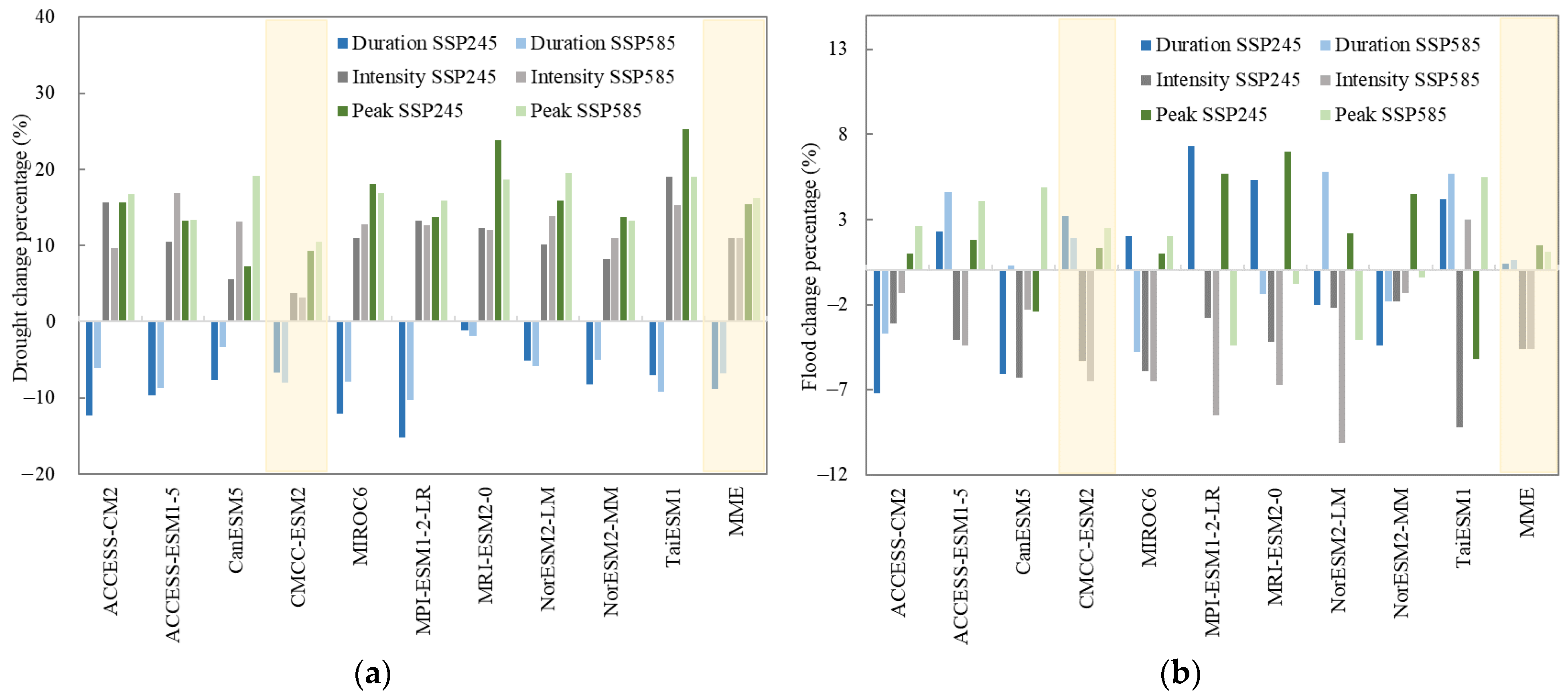
- Both the MME and the optimal model projected that the drought duration in the study area would decrease, especially after 2050, while the drought intensity and drought peak would increase overall under both scenarios, no matter the multi-year average level or the specific time period. It indicates that the duration of drought events in the future will be shortened, but drought will become more severe, and the magnitude of extreme drought will increase.
- (3)
- Both the MME and the optimal model projected the multi-year average flood intensity would decrease, while the flood duration and flood peak would increase on the whole under both scenarios, and that the increase magnitudes would be greater after 2080. It indicates that floods will become more severe after the mid- to late 21st century, with longer durations and a higher peak for flood events.
- (4)
- The MME and the optimal model projected the most similar trends for the duration, intensity, and peak of hydrological drought and floods in either the multi-year average level or in the specific time periods, although the magnitudes of the trends they projected vary.
Author Contributions
Funding
Institutional Review Board Statement
Informed Consent Statement
Data Availability Statement
Acknowledgments
Conflicts of Interest
References
- Alfieri, L.; Bisselink, B.; Dottori, F.; Naumann, G.; de Roo, A.; Salamon, P.; Wyser, K.; Feyen, L. Global projections of river flood risk in a warmer world. Earth’s Future 2017, 5, 171–182. [Google Scholar] [CrossRef]
- Cook, B.I.; Mankin, J.S.; Marvel, K.; Williams, A.P.; Smerdon, J.E.; Anchukaitis, K.J. Twenty-first century drought projections in the CMIP6 forcing scenarios. Earth’s Future 2020, 8, e2019EF001461. [Google Scholar] [CrossRef]
- Zhang, R.; Qu, Y.; Zhang, X.; Wu, X.; Zhou, X.; Ren, B.; Zeng, J.; Wang, Q. Spatiotemporal variability in annual drought severity, duration, and frequency from 1901 to 2020. Clim. Res. 2022, 87, 81–97. [Google Scholar] [CrossRef]
- Xu, Y.; Zhu, X.; Cheng, X.; Gun, Z.; Lin, J.; Zhao, J.; Yao, L.; Zhou, C. Drought assessment of China in 2002–2017 based on a comprehensive drought index. Agric. For. Meteorol. 2022, 319, 108922. [Google Scholar] [CrossRef]
- Bi, W.; Li, M.; Weng, B.; Yan, D.; Dong, Z.; Feng, J.; Wang, H. Drought-flood abrupt alteration events over China. Sci. Total Environ. 2023, 875, 162529. [Google Scholar] [CrossRef] [PubMed]
- Rezvani, R.; RahimiMovaghar, M.; Na, W.; Najafi, M.R. Accelerated lagged compound floods and droughts in northwest North America under 1.5 °C–4 °C global warming levels. J. Hydrol. 2023, 624, 129906. [Google Scholar] [CrossRef]
- Pavur, G.; Lakshmi, V. Observing the recent floods and drought in the Lake Victoria Basin using Earth observations and hydrological anomalies. J. Hydrol. Reg. Stud. 2023, 46, 101347. [Google Scholar] [CrossRef]
- Ye, Y.; Li, Z.; Li, X.; Li, Z. Projection and analysis of floods in the upper Heihe River basin under climate change. Atmosphere 2023, 14, 1083. [Google Scholar] [CrossRef]
- Tian, Q.; Li, Z.; Sun, X. Frequency analysis of precipitation extremes under a changing climate: A case study in Heihe River basin, China. J. Water Clim. Chang. 2021, 12, 772–786. [Google Scholar] [CrossRef]
- Gao, N.N.; Li, F.; Zeng, H.; Zheng, Y.R. The impact of human activities, natural factors, and climate time-lag effects over 33 years in the Heihe River Basin, China. Appl. Ecol. Environ. Res. 2021, 19, 1589–1606. [Google Scholar] [CrossRef]
- Hu, J.; Wu, Y.; Zhao, W.; Wang, F.; Zhang, G.; Qiu, L.; Hui, J.; Yin, X. Assessment and projection of ground freezing–thawing responses to climate change in the Upper Heihe River Basin, Northwest China. J. Hydrol. Reg. Stud. 2022, 42, 101137. [Google Scholar] [CrossRef]
- Li, Z.; Li, W.; Li, Z.; Lv, X. Responses of Runoff and Its Extremes to Climate Change in the Upper Catchment of the Heihe River Basin, China. Atmosphere 2023, 14, 539. [Google Scholar] [CrossRef]
- Yang, H.; Ma, F.; Yuan, X. The role of human activities in the weakening of the propagation relationship between meteorological and hydrological droughts in the Heihe River Basin. Hydrol. Process. 2023, 37, e14946. [Google Scholar] [CrossRef]
- Zhang, A.; Liu, W.; Yin, Z.; Fu, G.; Zheng, C. How will climate change affect the water availability in the Heihe River Basin, Northwest China? J. Hydrometeorol. 2016, 17, 1517–1542. [Google Scholar] [CrossRef]
- Luo, K.; Tao, F.; Moiwo, J.P.; Xiao, D. Attribution of hydrological change in Heihe River Basin to climate and land use change in the past three decades. Sci. Rep. 2016, 6, 33704. [Google Scholar] [CrossRef] [PubMed]
- Shang, X.; Jiang, X.; Jia, R.; Wei, C. Land use and climate change effects on surface runoff variations in the upper Heihe River basin. Water 2019, 11, 344. [Google Scholar] [CrossRef]
- Yin, Z.; Feng, Q.; Zou, S.; Yang, L. Assessing variation in water balance components in mountainous inland river basin experiencing climate change. Water 2016, 8, 472. [Google Scholar] [CrossRef]
- Yang, L.; Feng, Q.; Yin, Z.; Wen, X.; Si, J.; Li, C.; Deo, R.C. Identifying separate impacts of climate and land use/cover change on hydrological processes in upper stream of Heihe River, Northwest China. Hydrol. Process. 2017, 31, 1100–1112. [Google Scholar] [CrossRef]
- Wu, F.; Zhan, J.; Su, H.; Yan, H.; Ma, E. Scenario-based impact assessment of land use/cover and climate changes on watershed hydrology in Heihe River Basin of northwest China. Adv. Meteorol. 2015, 2015, 410198. [Google Scholar] [CrossRef]
- Li, Z.; Li, Q.; Wang, J.; Feng, Y.; Shao, Q. Impacts of projected climate change on runoff in upper reach of Heihe River basin using climate elasticity method and GCMs. Sci. Total Environ. 2020, 716, 137072. [Google Scholar] [CrossRef]
- Wang, Y.; Wang, Y.; Xu, H. Impacts of 1.5 °C and 2.0 °C global warming on runoff of three inland rivers in the Hexi Corridor, Northwest China. J. Meteorol. Res. 2020, 34, 1082–1095. [Google Scholar] [CrossRef]
- Cao, L.; Dou, Y.X.; Zhang, D.Y. Effect of Climate Change on Ecological Environment of Heihe Field. Arid Meteorol. 2003, 21, 45. [Google Scholar]
- Ren, Z.; Lu, Y.; Yang, D. Study on drought and flood changes in recent 2000 years in Heihe River Basin. J. Arid Land Resour. Environ. 2009, 23, 90–93. [Google Scholar]
- Li, M.-J.; Shi, P.-J. Climate Changing Characteristics of Zhangye City in Heihe River Basin During 1968–2005. J. Desert Res. 2007, 2007, 1048–1054. [Google Scholar] [CrossRef]
- Van Huijgevoort, M.H.J.; Van Lanen, H.A.J.; Teuling, A.J.; Uijlenhoet, R. Identification of changes in hydrological drought characteristics from a multi-GCM driven ensemble constrained by observed discharge. J. Hydrol. 2014, 512, 421–434. [Google Scholar] [CrossRef]
- Kamruzzaman, M.; Jang, M.W.; Cho, J.; Hwang, S. Future changes in precipitation and drought characteristics over Bangladesh under CMIP5 climatological projections. Water 2019, 11, 2219. [Google Scholar] [CrossRef]
- Yao, N.; Li, L.; Feng, P.; Feng, H.; Li Liu, D.; Liu, Y.; Jiang, K.; Hu, X.; Li, Y. Projections of drought characteristics in China based on a standardized precipitation and evapotranspiration index and multiple GCMs. Sci. Total Environ. 2020, 704, 135245. [Google Scholar] [CrossRef]
- Raje, D.; Mujumdar, P.P. Hydrologic drought prediction under climate change: Uncertainty modeling with Dempster–Shafer and Bayesian approaches. Adv. Water Resour. 2010, 33, 1176–1186. [Google Scholar] [CrossRef]
- Akhter, J.; Das, L.; Deb, A. CMIP5 ensemble-based spatial rainfall projection over homogeneous zones of India. Clim. Dyn. 2017, 49, 1885–1916. [Google Scholar] [CrossRef]
- Bisht, D.S.; Sridhar, V.; Mishra, A.; Chatterjee, C.; Raghuwanshi, N.S. Drought characterization over India under projected climate scenario. Int. J. Climatol. 2019, 39, 1889–1911. [Google Scholar] [CrossRef]
- Sung, J.H.; Park, J.; Jeon, J.J.; Seo, S.B. Assessment of inter-model variability in meteorological drought characteristics using CMIP5 GCMs over South Korea. KSCE J. Civ. Eng. 2020, 24, 2824–2834. [Google Scholar] [CrossRef]
- Shiru, M.S.; Chung, E.S.; Shahid, S.; Alias, N. GCM selection temperature projection of Nigeria under different RCPs of the CMIP5 GCMS. Theor. Appl. Climatol. 2020, 141, 1611–1627. [Google Scholar] [CrossRef]
- Chhin, R.; Oeurng, C.; Yoden, S. Drought projection in the Indochina Region based on the optimal ensemble subset of CMIP5 models. Clim. Chang. 2020, 162, 687–705. [Google Scholar] [CrossRef]
- Han, R.C.; Li, Z.L.; Han, Y.Y.; Huo, P.Y. A comparative study of TOPSIS-based GCMs selection and multi-model ensemble. Int. J. Climatol. 2023, 43, 5348–5368. [Google Scholar] [CrossRef]
- Wang, J.; Li, Z.L. Application of entropy weighted TOPSIS method for selection of general circulation models. South-North Water Transf. Water Sci. Technol. 2020, 18, 14–21. (In Chinese) [Google Scholar]
- Moriasi, D.N.; Arnold, J.G.; Van Liew, M.W.; Bingner, R.L.; Harmel, R.D.; Veith, T.L. Model evaluation guidelines for systematic quantification of accuracy in watershed simulations. Trans. ASABE 2007, 50, 885–900. [Google Scholar] [CrossRef]
- Piani, C.; Haerter, J.O.; Coppola, E. Statistical bias correction for daily precipitation in regional climate models over Europe. Theor. Appl. Climatol. 2010, 99, 187–192. [Google Scholar] [CrossRef]
- Teutschbein, C.; Seibert, J. Bias correction of regional climate model simulations for hydrological climate-change impact studies: Review and evaluation of different methods. J. Hydrol. 2012, 456, 12–29. [Google Scholar] [CrossRef]
- Ghimire, U.; Srinivasan, G.; Agarwal, A. Assessment of rainfall bias correction techniques for improved hydrological simulation. Int. J. Climatol. 2019, 39, 2386–2399. [Google Scholar] [CrossRef]
- Enayati, M.; Bozorg-Haddad, O.; Bazrafshan, J.; Hejabi, S.; Chu, X. Bias correction capabilities of quantile mapping methods for rainfall and temperature variables. J. Water Clim. Chang. 2021, 12, 401–419. [Google Scholar] [CrossRef]
- Li, X.T.; Li, Z.L.; Han, R.C. Evaluations of Different Bias Correction Methods on the GCM Precipitation Data. J. China Hydrol. 2023, 43, 93–111. (In Chinese) [Google Scholar]
- Wu, J.; Miao, C.; Tang, X.; Duan, Q.; He, X. A nonparametric standardized runoff index for characterizing hydrological drought on the Loess Plateau, China. Glob. Planet. Chang. 2018, 161, 53–65. [Google Scholar] [CrossRef]
- Sun, X.; Li, Z.; Tian, Q. Assessment of hydrological drought based on nonstationary runoff data. Hydrol. Res. 2020, 51, 894–910. [Google Scholar] [CrossRef]
- Porhemmat, J.; Altafi Dadgar, M. Analysis of hydrological drought indices in Alpine Zagros Mountains of Iran. Arab. J. Geosci. 2023, 16, 594. [Google Scholar] [CrossRef]
- Zan, D.W. Spatial-temporal variation characteristics of meteorological drought during 1967–2009 in the Heihe River Basin. J. Water Resour. Water Eng. 2019, 3, 92–99. [Google Scholar]


| Data | Spatial and Temporal Resolution | Data Source |
|---|---|---|
| DEM | 90 m | http://www.gscloud.cn/ (accessed on 26 March 2021) |
| Land use type data | 1 km | https://www.resdc.cn/DOI/DOI.aspx?DOIID=54 (accessed on 26 March 2021) |
| Soil data | 1 km | http://www.fao.org/soils-portal/soil-survey/soil-maps-and-databases/harmonized-world-soil-database-v12/en/ (accessed on 19 April 2021) |
| Meteorological data | 1987–2014, daily | http://data.cma.cn/site/index.html (accessed on 19 April 2021) |
| Runoff data | 1987–2014, daily | Hydrologic manual |
| Station Type | Station Name | Longitude (°) | Latitude (°) |
|---|---|---|---|
| Meteorological station | Tuole | 38.8 | 98.42 |
| Yeniugou | 38.42 | 99.58 | |
| Qilian | 38.18 | 100.25 | |
| Hydrological station | Yingluoxia | 38.82 | 100.18 |
| GCM | Organization | Spatial and Temporal Resolution |
|---|---|---|
| ACCESS-CM2 | Commonwealth Scientific and Industrial Research Organization and Australian Research Council Centre of Excellence for Climate System Science | 1.875° × 1.25°, daily |
| ACCESS-ESM1-5 | 1.875° × 1.25°, daily | |
| CanESM5 | Canadian Centre for Climate Modelling and Analysis | 2.8125° × 2.8125°, daily |
| CMCC-ESM2 | Euro-Mediterranean Centre on Climate Change | 1.25° × 0.9375°, daily |
| MIROC6 | Japan Agency for Marine-Earth Science and Technology | 1.40625° × 1.40625°, daily |
| MPI-ESM1-2-LR | Max Planck Institute for Meteorology | 1.875° × 1.875°, daily |
| MRI-ESM2-0 | Meteorological Research Institute | 1.125° × 1.125°, daily |
| NorESM2-LM | Norwegian Climate Service Centre | 2.5° × 1.875°, daily |
| NorESM2-MM | 1.25° × 0.9375°, daily | |
| TaiESM | Research Center for Environmental Changes, Academia Sinica | 1.25° × 0.9375°, daily |
| Model Performance | ||
|---|---|---|
| Very good | 0.75–1.00 | 0.75–1.00 |
| Good | 0.65–0.75 | 0.65–0.75 |
| Satisfactory | 0.50–0.65 | 0.50–0.65 |
| Not satisfactory | <0.50 | <0.50 |
| GCM | Precipitation (mm) | Maximum Temperature (°C) | Minimum Temperature (°C) | Relative Humidity (%) | Wind Speed (m/s) | |||||
|---|---|---|---|---|---|---|---|---|---|---|
| Before | After | Before | After | Before | After | Before | After | Before | After | |
| ACCESS-CM2 | 2.45 | −0.04 | 0.67 | 0.00 | 1.59 | 0.00 | 0.49 | 0.00 | −0.12 | 0.00 |
| ACCESS-ESM1-5 | 2.63 | −0.02 | 1.08 | 0.00 | 2.18 | 0.00 | 0.61 | 0.00 | 0.03 | 0.00 |
| CanESM5 | 2.39 | 0.05 | 0.91 | 0.00 | 1.87 | 0.00 | 0.41 | 0.00 | 0.31 | 0.00 |
| CMCC-ESM2 | 2.39 | 0.03 | 1.18 | 0.00 | 1.80 | 0.00 | 0.47 | 0.00 | −0.21 | 0.00 |
| MIROC6 | 2.35 | −0.08 | 1.01 | 0.00 | 1.95 | 0.00 | 0.47 | 0.00 | −0.13 | 0.01 |
| MPI-ESM1-2-LR | 2.47 | 0.01 | 0.56 | 0.00 | 1.64 | 0.00 | 0.62 | 0.00 | 0.82 | 0.00 |
| MRI-ESM2-0 | 2.62 | −0.06 | 0.87 | 0.00 | 1.82 | 0.00 | 0.36 | 0.00 | 0.47 | 0.00 |
| NorESM2-LM | 2.11 | 0.02 | 1.18 | 0.00 | 1.98 | 0.00 | 0.33 | 0.00 | 0.34 | 0.00 |
| NorESM2-MM | 2.13 | −0.01 | 1.19 | 0.00 | 1.90 | 0.00 | 0.30 | 0.00 | 0.26 | 0.00 |
| TaiESM1 | 2.24 | 0.01 | 1.18 | 0.00 | 1.63 | 0.00 | 0.40 | 0.00 | −0.22 | 0.00 |
| Meteorological Variables | GCM | Difference in Mean | Difference in Standard Deviation | Difference in Coefficient of Variation | Normalized Root Mean Square Error | Pearson Correlation Coefficient |
|---|---|---|---|---|---|---|
| Precipitation | ACCESS-CM2 | 1.223 | 5.228 | 0.122 | 0.575 | 0.820 |
| ACCESS-ESM1-5 | 0.714 | 0.601 | 0.005 | 0.028 | 0.982 | |
| CanESM5 | 2.181 | 0.251 | 0.059 | 0.006 | 0.997 | |
| CMCC-ESM2 | 0.763 | 0.238 | 0.030 | 0.024 | 0.985 | |
| MIROC6 | 3.368 | 3.885 | 0.016 | 0.019 | 0.986 | |
| MPI-ESM1-2-LR | 2.778 | 3.062 | 0.009 | 0.030 | 0.977 | |
| MRI-ESM2-0 | 2.285 | 1.017 | 0.042 | 0.038 | 0.974 | |
| NorESM2-LM | 2.575 | 1.721 | 0.030 | 0.090 | 0.939 | |
| NorESM2-MM | 0.984 | 1.570 | 0.018 | 0.003 | 0.998 | |
| TaiESM1 | 0.668 | 2.681 | 0.062 | 0.067 | 0.948 | |
| Maximum Temperature | ACCESS-CM2 | 0.013 | 0.073 | 0.011 | 0.260 | 0.967 |
| ACCESS-ESM1-5 | 0.011 | 0.035 | 0.006 | 0.008 | 0.998 | |
| CanESM5 | 0.011 | 0.046 | 0.004 | 0.015 | 0.997 | |
| CMCC-ESM2 | 0.001 | 0.019 | 0.002 | 0.006 | 0.999 | |
| MIROC6 | 0.012 | 0.085 | 0.009 | 0.028 | 0.993 | |
| MPI-ESM1-2-LR | 0.009 | 0.081 | 0.009 | 0.007 | 0.999 | |
| MRI-ESM2-0 | 0.010 | 0.013 | 0.000 | 0.021 | 0.995 | |
| NorESM2-LM | 0.006 | 0.041 | 0.004 | 0.021 | 0.995 | |
| NorESM2-MM | 0.009 | 0.009 | 0.002 | 0.020 | 0.995 | |
| TaiESM1 | 0.016 | 0.047 | 0.004 | 0.013 | 0.997 | |
| Minimum Temperature | ACCESS-CM2 | 0.008 | 0.085 | 0.011 | 0.198 | 0.980 |
| ACCESS-ESM1-5 | 0.023 | 0.022 | 0.001 | 0.016 | 0.997 | |
| CanESM5 | 0.020 | 0.024 | 0.006 | 0.010 | 0.998 | |
| CMCC-ESM2 | 0.007 | 0.002 | 0.001 | 0.007 | 0.999 | |
| MIROC6 | 0.011 | 0.074 | 0.007 | 0.019 | 0.996 | |
| MPI-ESM1-2-LR | 0.006 | 0.074 | 0.008 | 0.010 | 0.998 | |
| MRI-ESM2-0 | 0.006 | 0.001 | 0.001 | 0.008 | 0.999 | |
| NorESM2-LM | 0.001 | 0.023 | 0.003 | 0.007 | 0.999 | |
| NorESM2-MM | 0.005 | 0.030 | 0.003 | 0.005 | 0.999 | |
| TaiESM1 | 0.005 | 0.052 | 0.006 | 0.008 | 0.998 |
| Evaluation Indicators | Precipitation | Maximum Temperature | Minimum Temperature |
|---|---|---|---|
| Mean | 0.087 | 0.093 | 0.072 |
| Standard deviation | 0.068 | 0.109 | 0.103 |
| Coefficient of variation | 0.051 | 0.091 | 0.070 |
| Normalized root mean square error | 0.042 | 0.042 | 0.042 |
| Pearson correlation coefficient | 0.045 | 0.043 | 0.042 |
| GCM | Rank | GCM | Rank | ||
|---|---|---|---|---|---|
| ACCESS-CM2 | 0.27 | 10 | MPI-ESM1-2-LR | 0.43 | 8 |
| ACCESS-ESM1-5 | 0.64 | 5 | MRI-ESM2-0 | 0.74 | 3 |
| CanESM5 | 0.57 | 6 | NorESM2-LM | 0.66 | 4 |
| CMCC-ESM2 | 0.89 | 1 | NorESM2-MM | 0.76 | 2 |
| MIROC6 | 0.37 | 9 | TaiESM1 | 0.56 | 7 |
| GCM | SSP245 | SSP585 | ||
|---|---|---|---|---|
| Runoff (m3/s) | Change Rate (%) | Runoff (m3/s) | Change Rate (%) | |
| ACCESS-CM2 | 45.0 | 10.8 | 46.5 | 14.5 |
| ACCESS-ESM1-5 | 40.2 | −0.9 | 40.2 | −0.9 |
| CanESM5 | 40.2 | −1.0 | 41.0 | 1.0 |
| CMCC-ESM2 | 37.7 | −7.1 | 37.3 | −8.1 |
| MIROC6 | 42.0 | 3.6 | 41.4 | 2.0 |
| MPI-ESM1-2-LR | 35.3 | −13.0 | 37.3 | −8.2 |
| MRI-ESM2-0 | 42.4 | 4.4 | 48.6 | 19.8 |
| NorESM2-LM | 43.7 | 7.7 | 44.3 | 9.1 |
| NorESM2-MM | 37.3 | −8.2 | 36.1 | −11.0 |
| TaiESM1 | 41.2 | 1.6 | 42.3 | 4.4 |
| MME | 40.5 | —— | 41.5 | 2.3% |
| Variables | MME | CMCC-ESM2 | |||
|---|---|---|---|---|---|
| SSP245 | SSP585 | SSP245 | SSP585 | ||
| Runoff | 0.0 | −7.1 | 2.3 | −8.1 | |
| Hydrological drought | Duration | −8.8 | −6.8 | −6.7 | −8.0 |
| Intensity | 11.0 | 11.0 | 3.8 | 3.2 | |
| Peak | 15.4 | 16.2 | 9.3 | 10.5 | |
| Flood | Duration | 0.4 | 0.6 | 3.2 | 1.9 |
| Intensity | −4.6 | −4.6 | −5.3 | −6.5 | |
| Peak | 1.5 | 1.1 | 1.3 | 2.5 | |
| Hydrological Extreme | Scenario | Time Period | Duration | Intensity | Peak | |||
|---|---|---|---|---|---|---|---|---|
| CMCC-ESM2 | MME | CMCC-ESM2 | MME | CMCC-ESM2 | MME | |||
| Drought | SSP245 | 2026–2049 | 24.2 | 5.4 | 5.8 | 11.4 | 21.4 | 20.0 |
| 2050–2079 | −20.0 | −15.0 | 3.3 | 8.8 | 7.5 | 11.3 | ||
| 2080–2100 | −21.4 | −16.1 | 2.6 | 13.3 | −1.3 | 15.8 | ||
| 2050–2100 | −20.6 | −15.4 | 3.0 | 10.7 | 3.9 | 13.2 | ||
| SSP585 | 2026–2049 | 16.7 | 5.9 | 0.3 | 10.8 | 15.3 | 18.5 | |
| 2050–2079 | −9.2 | −8.0 | 12.2 | 9.5 | 22.6 | 14.5 | ||
| 2080–2100 | −33.2 | −19.5 | −6.2 | 17.0 | −11.7 | 15.9 | ||
| 2050–2100 | −19.3 | −12.7 | 4.5 | 12.6 | 8.2 | 15.1 | ||
| Flood | SSP245 | 2026–2049 | 5.4 | −8.6 | −3.7 | −1.7 | 1.9 | 1.7 |
| 2050–2079 | −2.7 | 2.4 | −11.2 | −9.7 | −5.4 | −3.0 | ||
| 2080–2100 | 9.2 | 7.6 | 1.4 | −0.7 | 10.4 | 7.8 | ||
| 2050–2100 | 2.2 | 4.6 | −6.1 | −6.0 | 1.1 | 1.4 | ||
| SSP585 | 2026–2049 | −6.8 | −11.5 | −10.6 | −6.9 | −1.9 | −2.9 | |
| 2050–2079 | 7.5 | 0.5 | −1.6 | −4.8 | 10.6 | 0.4 | ||
| 2080–2100 | 3.7 | 14.8 | −8.9 | −1.7 | −4.4 | 6.8 | ||
| 2050–2100 | 5.9 | 6.3 | −4.6 | −3.5 | 4.5 | 3.1 | ||
| GCM | Precipitation (mm) | Maximum Temperature (°C) | Minimum Temperature (°C) | Relative Humidity (%) | Wind Speed (m/s) | |||||
|---|---|---|---|---|---|---|---|---|---|---|
| SSP245 | SSP585 | SSP245 | SSP585 | SSP245 | SSP585 | SSP245 | SSP585 | SSP245 | SSP585 | |
| ACCESS-CM2 | 414.5 | 430.4 | 10.4 | 11.6 | −6.0 | −5.0 | 0.51 | 0.50 | 2.26 | 2.24 |
| 6.9% ↑ | 11.1% ↑ | 2.4 °C ↑ | 3.5 °C ↑ | 2.3 °C ↑ | 3.3 °C ↑ | 5.6% ↓ | 7.4% ↓ | 1.3% ↑ | —— | |
| ACCESS-ESM1-5 | 397.9 | 393.3 | 10.9 | 11.7 | −5.7 | −4.8 | 0.51 | 0.51 | 2.18 | 2.14 |
| 2.7% ↑ | 1.5% ↑ | 2.9 °C ↑ | 3.7 °C ↑ | 2.6 °C ↑ | 3.5 °C ↑ | 5.6% ↓ | 5.6% ↓ | 2.2% ↓ | 4.0% ↓ | |
| CanESM5 | 429.6 | 439.0 | 10.7 | 12.0 | −5.8 | −4.5 | 0.54 | 0.54 | 1.99 | 1.93 |
| 10.8% ↑ | 13.3% ↑ | 2.7 °C ↑ | 3.9 °C ↑ | 2.6 °C ↑ | 3.9 °C ↑ | —— | —— | 10.8% ↓ | 13.5% ↓ | |
| CMCC-ESM2 | 429.8 | 468.3 | 10.69 | 11.1 | −5.9 | −5.1 | 0.53 | 0.54 | 2.03 | 2.03 |
| 10.9% ↑ | 20.8% ↑ | 2.7 °C ↑ | 3.1 °C ↑ | 2.5 °C ↑ | 3.2 °C ↑ | 1.9% ↓ | —— | 9.0% ↓ | 9.0% ↓ | |
| MIROC6 | 374.2 | 395.3 | 10.29 | 11.1 | −6.0 | −5.1 | 0.53 | 0.52 | 1.85 | 2.16 |
| 3.4% ↓ | 2.0% ↑ | 2.3 °C ↑ | 3.1 °C ↑ | 2.3 °C ↑ | 3.2 °C ↑ | 1.9% ↓ | 3.7% ↓ | 17.0% ↓ | 3.1% ↓ | |
| MPI-ESM1-2-LR | 416.2 | 426.1 | 9.5 | 10.5 | −6.8 | −5.9 | 0.52 | 0.51 | 2.07 | 2.16 |
| 7.4% ↑ | 9.9% ↑ | 1.5 °C ↑ | 2.4 °C ↑ | 1.6 °C ↑ | 2.5 °C ↑ | 3.7% ↓ | 5.6% ↓ | 7.2% ↓ | 3.1% ↓ | |
| MRI-ESM2-0 | 402.4 | 397.8 | 10.2 | 10.9 | −6.4 | −5.5 | 0.55 | 0.54 | 2.04 | 2.18 |
| 3.8% ↑ | 2.6% ↑ | 2.1 °C ↑ | 2.8 °C ↑ | 1.9 °C ↑ | 2.9 °C ↑ | 1.9% ↑ | —— | 8.5% ↓ | 2.2% ↓ | |
| NorESM2-LM | 405.9 | 410.1 | 10.3 | 11.3 | −6.4 | −5.2 | 0.52 | 0.51 | 2.02 | 1.98 |
| 4.7% ↑ | 5.8% ↑ | 2.3 °C ↑ | 3.2 °C ↑ | 2.0 °C ↑ | 3.1 °C ↑ | 3.7% ↓ | 5.6% ↓ | 9.4% ↓ | 11.2% ↓ | |
| NorESM2-MM | 406.5 | 408.9 | 10.1 | 10.9 | −6.5 | −5.5 | 0.53 | 0.53 | 2.02 | 1.99 |
| 4.9% ↑ | 5.5% ↑ | 2.0 °C ↑ | 2.9 °C ↑ | 1.8 °C ↑ | 2.9 °C ↑ | 1.9% ↓ | 1.9% ↓ | 9.4% ↓ | 10.8% ↓ | |
| TaiESM1 | 440.3 | 429.7 | 11.1 | 6.3 | −6.0 | −4.6 | 0.52 | 0.51 | 2.26 | 2.26 |
| 13.6% ↑ | 10.9% ↑ | 3.0 °C ↑ | −1.7 °C ↓ | 2.4 °C ↑ | 3.8 °C ↑ | 3.7% ↓ | 5.6% ↓ | 1.3% ↑ | 1.3% ↑ | |
| MME | 411.7 | 419.9 | 10.4 | 10.7 | −6.1 | −5.1 | 0.53 | 0.52 | 2.07 | 2.11 |
| 6.2% ↑ | 8.3% ↑ | 2.4 °C ↑ | 2.7 °C ↑ | 2.3 °C ↑ | 3.3 °C ↑ | 1.9% ↓ | 3.7% ↓ | 7.2% ↓ | 5.4% ↓ | |
Disclaimer/Publisher’s Note: The statements, opinions and data contained in all publications are solely those of the individual author(s) and contributor(s) and not of MDPI and/or the editor(s). MDPI and/or the editor(s) disclaim responsibility for any injury to people or property resulting from any ideas, methods, instructions or products referred to in the content. |
© 2024 by the authors. Licensee MDPI, Basel, Switzerland. This article is an open access article distributed under the terms and conditions of the Creative Commons Attribution (CC BY) license (https://creativecommons.org/licenses/by/4.0/).
Share and Cite
Li, Z.; Ye, Y.; Lv, X.; Bai, M.; Li, Z. Hydrological Drought and Flood Projection in the Upper Heihe River Basin Based on a Multi-GCM Ensemble and the Optimal GCM. Atmosphere 2024, 15, 439. https://doi.org/10.3390/atmos15040439
Li Z, Ye Y, Lv X, Bai M, Li Z. Hydrological Drought and Flood Projection in the Upper Heihe River Basin Based on a Multi-GCM Ensemble and the Optimal GCM. Atmosphere. 2024; 15(4):439. https://doi.org/10.3390/atmos15040439
Chicago/Turabian StyleLi, Zhanling, Yingtao Ye, Xiaoyu Lv, Miao Bai, and Zhanjie Li. 2024. "Hydrological Drought and Flood Projection in the Upper Heihe River Basin Based on a Multi-GCM Ensemble and the Optimal GCM" Atmosphere 15, no. 4: 439. https://doi.org/10.3390/atmos15040439
APA StyleLi, Z., Ye, Y., Lv, X., Bai, M., & Li, Z. (2024). Hydrological Drought and Flood Projection in the Upper Heihe River Basin Based on a Multi-GCM Ensemble and the Optimal GCM. Atmosphere, 15(4), 439. https://doi.org/10.3390/atmos15040439