
The Effects of Lockdown, Urban Meteorology, Pollutants, and Anomalous Diffusion on the SARS-CoV-2 Pandemic in Santiago de Chile


Abstract
1. Introduction
2. Materials and Methods
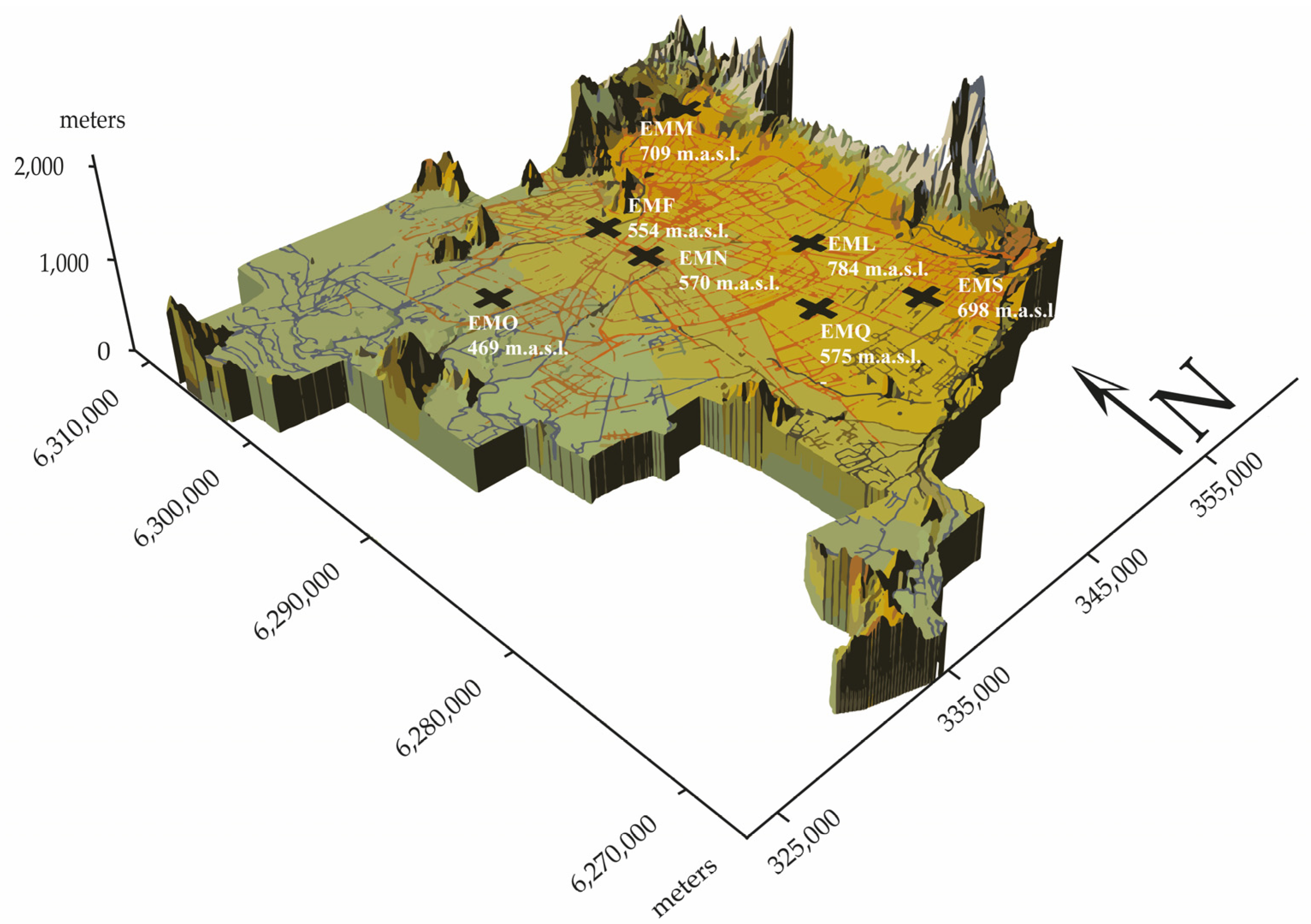
2.1. Area of Study
2.2. The Data
2.2.1. PM2.5 and PM10 Particulate Matter
2.2.2. Tropospheric Ozone (O3)
2.2.3. Meteorological Variables
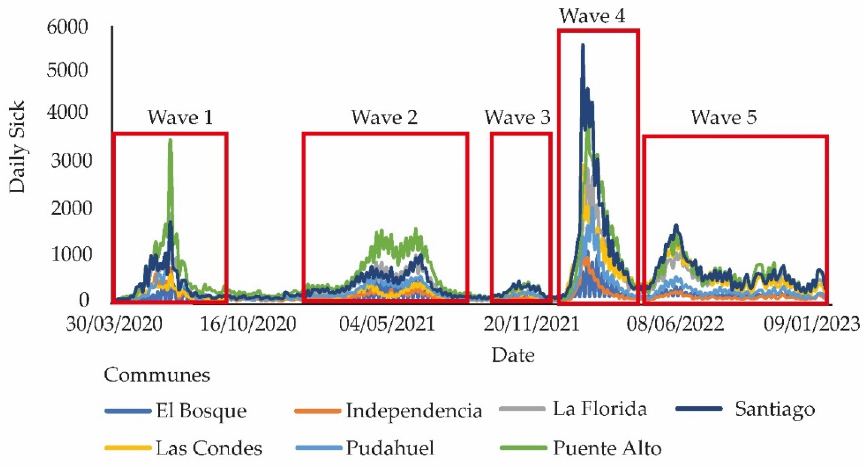
2.2.4. COVID-19 in Santiago de Chile
Waves
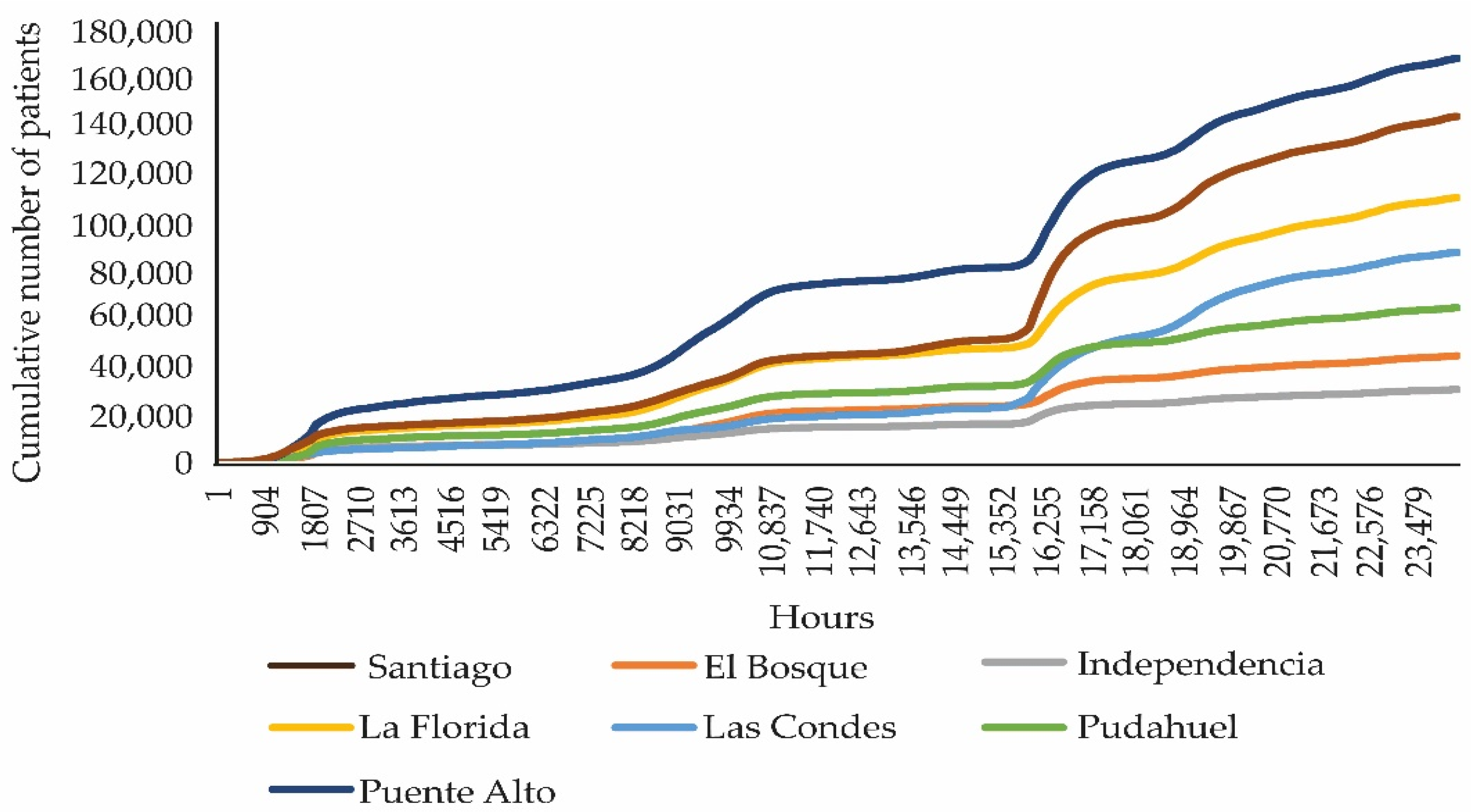
Cumulative Sick Data
2.3. Mathematical Tools
2.3.1. Chaos Theory
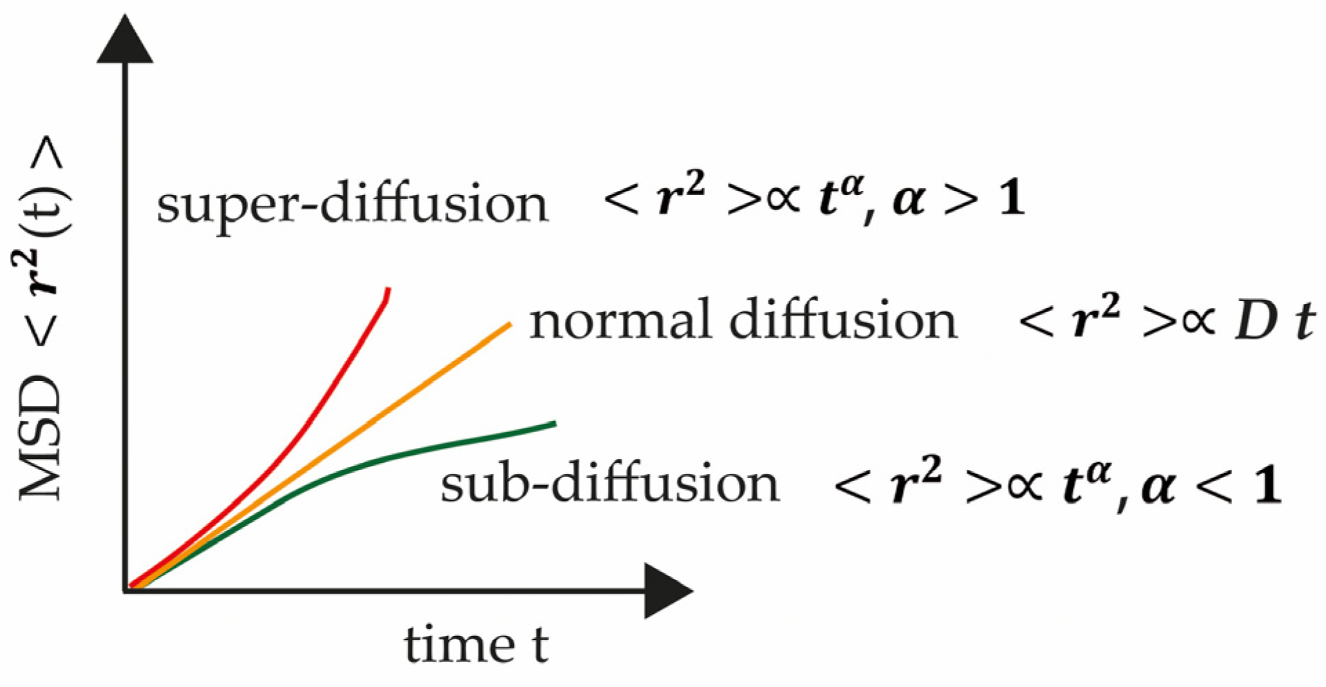
2.3.2. Anomalous Diffusion
3. Results
4. Discussion
5. Conclusions
Author Contributions
Funding
Institutional Review Board Statement
Informed Consent Statement
Data Availability Statement
Acknowledgments
Conflicts of Interest
References
- Pacheco, P.; Mera, E.; Fuentes, V. Intensive Urbanization, Urban Meteorology and Air Pollutants: Effects on the Temperature of a City in a Basin Geography. Int. J. Environ. Res. Public Health 2023, 20, 3941. [Google Scholar] [CrossRef] [PubMed]
- Pacheco, P.; Mera, E. Relations between Urban Entropies, Geographical Configurations, Habitability and Sustainability. Atmosphere 2022, 13, 1639. [Google Scholar] [CrossRef]
- Salini, G.A.; Pacheco, P.R.; Mera, E.; Parodi, M.C. Probable relationship between COVID-19, pollutants and meteorology: A case study at Santiago, Chile. Aerosol Air Qual. Res. 2021, 21, 200434. [Google Scholar] [CrossRef]
- Pacheco, P.; Mera, E. Study of the Effect of Urban Densification and Micrometeorology on the Sustainability of a Coronavirus-Type Pandemic. Atmosphere 2022, 13, 1073. [Google Scholar] [CrossRef]
- Neeltje van Doremalen, N.; Bushmaker, T.; Morris, D.H.; Holbrook, M.G.; Gamble, A.; Williamson, B.N.; Tamin, A.; Harcourt, J.L.; Thornburg, N.J.; Gerber, S.I.; et al. Aerosol and Surface Stability of SARS-CoV-2, as Compared with SARS-CoV-1. N. Engl. J. Med. 2020, 382, 1564–1567. [Google Scholar] [CrossRef]
- Gramsch, E.; Morales, L.; Baeza, M.; Ayala, C.; Soto, C.; Neira, J.; Pérez, P.; Moreno, F. Citizens’ Surveillance Micro-network for the Mapping of PM2.5 in the City of Concón, Chile. Aerosol Air Qual Res. 2020, 20, 358–368. [Google Scholar] [CrossRef]
- Đorđević, D.; Milanković, J.D.; Pantelić, A.; Petrović, S.; Gambaro, A. Coarse, fine and ultrafine particles of suburban-continental aerosols measured using an 11-stage Berner cascade impactor. Atmos. Pollut. Res. 2020, 11, 499–510. [Google Scholar] [CrossRef]
- Iwasaka, Y.; Minoura, H.; Nagaya, K. The transport and spacial scale of Asian dust-storm clouds: A case study of the dust-storm event of April 1979. Tellus B Chem. Phys. Meteorol. 1983, 35, 189–196. [Google Scholar] [CrossRef]
- WHO/Europe. Review of Evidence on Health Aspects of Air Pollution—REVIHAAP Project Technical Report; World Health Organization, Regional Office for Europe: Copenhagen, Denmark, 2013; Available online: https://www.eea.europa.eu/data-and-maps/indicators/exceedance-of-air-quality-limit-3/who-2013 (accessed on 27 November 2022).
- Nuvolone, D.; Petri, D.; Voller, F. The effects of ozone on human health. Environ. Sci. Pollut. Res. 2018, 25, 8074–8088. [Google Scholar] [CrossRef]
- Díaz, J.; Ortiz, C.; Falcón, I.; Salvador, C.; Linares, C. Short-term effect of tropospheric ozone on daily mortality in Spain. Atmos. Environ. 2018, 187, 107–116. [Google Scholar] [CrossRef]
- Byass, P. Eco-epidemiological assessment of the COVID-19 epidemic in China, January–February 2020. Glob. Health Action 2020, 13, 1760490. [Google Scholar] [CrossRef] [PubMed]
- Iqbal, N.; Fareed, Z.; Shahzad, F.; He, X.; Shahzad, U.; Lina, M. The nexus between COVID19, temperature and exchange rate in Wuhan city: New findings from partial and multiple wavelet coherence. Sci. Total Environ. 2020, 729, 138916. [Google Scholar] [CrossRef] [PubMed]
- MINSAL (Chilean Ministry of Health). Available online: https://www.minsal.cl/ (accessed on 15 January 2023).
- SINCA (Chilean Air Quality National Information System). Available online: https://sinca.mma.gob.cl (accessed on 30 January 2023).
- Silverman, B.W.; Jones, M.C.; Fix, E. An Important Contribution to Nonparametric Discriminant Analysis and Density Estimation: Commentary on Fix and Hodges (1951). Int. Stat. Rev. 1989, 57, 233–238. [Google Scholar] [CrossRef]
- Junninen, H.; Niska, H.; Tuppurainen, K.; Ruuskanen, J.; Kolehmainen, M. Methods for imputation of missing values in air quality data sets. Atmos. Environ. 2004, 38, 2895–2907. [Google Scholar] [CrossRef]
- Norazian, M.N.; Shruki, Y.A.; Azam, R.M.; Mustafa Al Bakri, A.M. Estimation of missing values in air pollution data using single imputation techniques. ScienceAsia 2008, 34, 341–345. [Google Scholar] [CrossRef]
- Emery, X. Simple and ordinary multigaussian Kriging for estimating recoverable reserves. Math. Geol. 2005, 37, 295–319. [Google Scholar] [CrossRef]
- Asa, E.; Saafi, M.; Membah, J.; Billa, A. Comparison of linear and nonlinear Kriging methods for characterization and interpolation of soil data. J. Comput. Civil Eng. 2012, 26, 11–18. [Google Scholar] [CrossRef]
- Pacheco, P.; Mera, E.; Salini, G. Medición Localizada de Contaminantes Atmosféricos y Variables Meteorológicas: Segunda Ley de la Termodinámica. Inf. Tecnol. 2019, 30, 105–116. [Google Scholar] [CrossRef][Green Version]
- Census. XIX Censo Nacional de Población y VIII de Vivienda o Censo de Población y Vivienda 2017, Gobierno de Chile e Instituto Nacional de Estadísticas de Chile. 2017. Available online: https://www.ine.cl (accessed on 23 November 2022).
- INE-Plataforma de Datos Estadísticos. Available online: https://www.ine.es/ine/planine/informe_anual_2019.pdf (accessed on 11 December 2022).
- MVU, Ministerio de Vivienda y Urbanismo (Ministry of Housing and Urbanism); Centro de Estudios de Ciudad y Territorio. Available online: https://www.observatoriourbano.cl (accessed on 3 January 2023).
- Government of Chile. Official Data COVID-19. Available online: https://www.gob.cl/coronavirus/cifrasoficiales/ (accessed on 18 January 2023).
- Salini, G.; Pérez, P. A study of the dynamic behavior of fine particulate matter in Santiago, Chile. Aerosol Air Qual. Res. 2015, 15, 154–165. [Google Scholar] [CrossRef]
- Sprott, J.C. Chaos and Time-Series Analysis, 1st ed.; Oxford University Press: Oxford, UK, 2003. [Google Scholar]
- Manríquez, R. Estructuras disipativas. De la termodinámica a la psicoterapia familiar. Rev. Asoc. Española Neuropsiquiatría 1987, VII, 435–454. [Google Scholar]
- Chen, Y.; Wang, J.; Feng, J. Understanding the Fractal Dimensions of Urban Forms through spatial. Entropy 2017, 19, 600. [Google Scholar] [CrossRef]
- Wolf, A.; Swift, J.B.; Swinney, H.L.; Vastano, J.A. Determining Lyapunov exponents from a time series. Phys. D 1985, 16, 285–317. [Google Scholar] [CrossRef]
- Grassberger, P.; Procaccia, L. Characterization of Strange Attractors. Phys. Rev. Lett. 1983, 50, 346–349. [Google Scholar] [CrossRef]
- Horna Mercedes, J.; Dionicio Vereau, J.; Martinez Zocón, R.; Zavaleta Quipuscoa, A.; Brenis Delgado, Y. Dinámica simbólica y algunas aplicaciones. Sel. Matemáticas 2016, 3, 101–106. [Google Scholar] [CrossRef]
- Sprott, J.C. Chaos Data Analyzer Software. 1995. Available online: http://sprott.physics.wisc.edu./cda.htm (accessed on 4 April 2023).
- Green, D.G. Connectivity and the evolution of biological systems. J. Biol. Syst. 1994, 2, 91–103. [Google Scholar] [CrossRef]
- Zellmer, A.J.; Wood, E.M.; Surasinghe, T.; Putman, B.J.; Pauly, G.B.; Magle, S.B.; Lewis, J.S.; Kay, C.A.M.; Fidino, M. What can we learn from wildlife sightings during the COVID-19 global shutdown? Ecosphere 2020, 11, e03215. [Google Scholar] [CrossRef]
- Sahin, O.; Salim, H.; Suprun, E.; Richards, R.; MacAskill, S.; Heilgeist, S.; Rutherford, S.; Stewart, R.A.; Beal, C.D. Developing a Preliminary Causal Loop Diagram for Understanding the Wicked Complexity of the COVID-19 Pandemic. Systems 2020, 8, 20. [Google Scholar] [CrossRef]
- Baker, R.E.; Yang, W.; Vecchi, G.A.; Metcalf, C.J.E.; Grenfell, B.T. Susceptible supply limits the role of climate in the COVID-19 pandemic. Science 2020, 369, 315–319. [Google Scholar] [CrossRef]
- Pacheco Hernández, P.R.; Salini Calderón, G.A.; Mera Garrido, E.M. Entropía y Neguentropía: Una aproximación al proceso de difusión de contaminantes y su sostenibilidad. Rev. Int. Contam. Ambient. 2021, 37, 167–185. [Google Scholar] [CrossRef]
- Lewis, D. What scientists have learnt from COVID lockdowns. Nature 2022, 609, 236–239. [Google Scholar] [CrossRef] [PubMed]
- Chen, S.; Guo, L.; Alghaith, T.; Dong, D.; Alluhidan, M.; Hamza, M.M.; Herbst, C.H.; Zhang, X.; Tagtag, G.C.A.; Zhang, Y.; et al. Effective COVID-19 Control: A Comparative Analysis of the Stringency and Timeliness of Government Responses in Asia. Int. J. Environ. Res. Public Health 2021, 18, 8686. [Google Scholar] [CrossRef]
- Wu, S.; Neill, R.; De Foo, C.; Chua, A.Q.; Jung, A.S.; Haldane, V.; Abdalla, S.M.; Guan, W.J.; Singh, S.; Nordström, A.; et al. Aggressive containment, suppression, and mitigation of COVID-19: Lessons learnt from eight countries. BMJ 2021, 375, e067508. [Google Scholar] [CrossRef]
- Li, Y.; Undurraga, E.A.; Zubizarreta, J.R. Effectiveness of Localized Lockdowns in the COVID-19 Pandemic. Am. J. Epidemiol. 2022, 191, 812–824. [Google Scholar] [CrossRef] [PubMed]
- Khalis, M.; Toure, A.B.; El Badisy, I.; Khomsi, K.; Najmi, H.; Bouaddi, O.; Marfak, A.; Al-Delaimy, W.K.; Berraho, M.; Nejjari, C. Relationship between Meteorological and Air Quality Parameters and COVID-19 in Casablanca Region, Morocco. Int. J. Environ. Res. Public Health 2022, 19, 4989. [Google Scholar] [CrossRef] [PubMed]
- Zhu, J.; Zhou, Y.; Lin, Q.; Wu, K.; Ma, Y.; Liu, C.; Liu, N.; Tu, T.; Liu, Q. Causal relationship between particulate matter and COVID-19 risk: A mendelian randomization study. Heliyon 2024, 24, e27083. [Google Scholar] [CrossRef] [PubMed]
- Fontanelli, O.; Mansilla, R.; Miramontes, P. Probability distributions in the complexity sciences: A contemporary perspective. Inter. Discip. 2020, 8, 11–37. [Google Scholar] [CrossRef]
- Shah, K.; Sinan, M.; Abdeljawad, T.; El-Shorbagy, M.A.; Abdalla, B.; Abualrub, M.S. A Detailed Study of a Fractal-Fractional Transmission Dynamical Model of Viral Infectious Disease with Vaccination. Complexity 2022, 2022, 7236824. [Google Scholar] [CrossRef]
- Sinan, M.; Alharthi, N.H. Mathematical Analysis of Fractal-Fractional Mathematical Model of COVID-19. Fractal Fract. 2023, 7, 358. [Google Scholar] [CrossRef]
- El-Borai, M.; El-Nadi, K. Stochastic Fractional Models of the Diffusion of COVID-19. Adv. Math. Sci. J. 2020, 9, 10281–10293. [Google Scholar] [CrossRef]


| Station Name | Geography | Climate | Pollution | Wind | T (°C)Average Period | RH (%)Average Period |
|---|---|---|---|---|---|---|
| 1. La Florida, EML, masl: 784 (m) | Located in the Andes piedmont | Cold, wet winters with little rainfall; hot and dry summers | Presence in descending order PM10, CO, PM2.5, NO2, O3, SO2 | West–east dayEast–west night | 15.33 | 58.85 |
| 2. Las Condes, EMM, masl: 709 (m) | Located in the Andes piedmont | Cold, dry winters; hot, dry summers | Presence in descending order PM10, CO, PM2.5, NO2, O3, SO2 | West–east dayEast–west night | 13.99 | 59.44 |
| 3. Santiago-Parque O’Higgins, EMN, masl: 570 (m) | Located in the middle of the basin plane | Cold, dry winters; hot, dry summers | Presence in descending order PM10, PM2.5, CO, SO2, NO2, O3 | West–east dayEast–south night | 15.26 | 63.20 |
| 4. Pudahuel, EMO, masl: 469 (m) | Located at the bottom of the basin | Cold, dry winters; hot, dry summers | Presence in descending order PM10, PM2.5, CO, SO2, NO2, O3 | South–east dayEast–south night | 14.51 | 63.89 |
| 5. Puente Alto, EMS, masl: 698 (m) | Located in the Andes piedmont | Cold, wet winters with moderate rainfall; hot, dry summers | Presence in descending order PM10, CO, PM2.5, NO2, O3, SO2 | West–east dayEast–west night | 14.68 | 58.92 |
| 6. Independencia, EMF, masl: 554 (m) | Situated in the intermediate zone of the basin | Cold, dry winters; hot, dry summers | Presence in descending order PM10, PM2.5, CO, SO2, NO2, O3 | North–east day East–south night | 15.17 | 61.18 |
| 7. El Bosque EMQ, masl: 575 (m) | Located at the bottom of the basin | Cold, wet winters; hot, dry summers | Presence in descending order PM10, PM2.5, NO2, CO, SO2, O3 | South–east dayEast–south night | 13.61 | 59.09 |
| Commune | Population | Accumulated Sick | People per Capita | Multidimensional Poverty |
|---|---|---|---|---|
| (2017) | (2017) | (31 March 2020–9 January 2023) | Income in USD | Index [22] |
| Santiago | 404,496 | 141,401 | 471 | 5–10% |
| Independencia | 100,281 | 29,960 | 127 | 20–25% |
| Las Condes | 294,838 | 85,890 | 1317 | <5% |
| Puente Alto | 568,106 | 165,038 | 175 | 20–25% |
| El Bosque | 162,505 | 43,638 | 188 | 20–25% |
| La Florida | 366,916 | 108,264 | 209 | 15–20% |
| Pudahuel | 230,293 | 63,290 | 335 | 20–25% |
| Total | 2,127,435 | 637,481 | 2822 |
| Commune | 2010 m2 | 2020 m2 | Δm2 | AS (31 March 2020–09 January 2023) | Inhabitant Density hab/km2 [22] |
|---|---|---|---|---|---|
| La Florida | 44,054 | 118,300 | 74,246 | 108,264 | 5227 |
| Las Condes | 127,342 | 145,306 | 17,964 | 85,890 | 2977 |
| Santiago | 94,043 | 190,862 | 96,819 | 141,401 | 17,436 |
| Pudahuel | 18,788 | 63,090 | 44,302 | 63,290 | 1000 |
| Puente Alto | 226,665 | 292,000 | 65,335 | 165,038 | 6456 |
| Pudahuel | Independencia | Santiago | Las Condes | La Florida | Pte. Alto | El Bosque | |
|---|---|---|---|---|---|---|---|
| Accum. sick | |||||||
| Deviation | 19,575.06 | 8798.44 | 45,046.67 | 27,671.65 | 33,137.88 | 50,748.94 | 13,660.27 |
| Average | 30,047.79 | 15,354.37 | 57,472.85 | 30,443.55 | 47,098.76 | 76,376.38 | 21,138.38 |
| Median | 28,463.00 | 14,611.00 | 43,992.00 | 19,391.00 | 42,991.00 | 73,636.00 | 21,357.00 |
| Temp (°C) | |||||||
| Deviation | 7.11 | 6.83 | 6.93 | 6.92 | 7.28 | 6.72 | 7.33 |
| Average | 14.51 | 15.17 | 15.26 | 13.99 | 15.33 | 14.68 | 13.61 |
| Median | 13.55 | 14.29 | 14.33 | 12.95 | 14.55 | 13.90 | 12.76 |
| RH (%) | |||||||
| Deviation | 22.45 | 21.48 | 21.91 | 21.10 | 21.27 | 20.83 | 21.55 |
| Average | 63.89 | 61.18 | 63.20 | 59.44 | 58.85 | 58.92 | 59.09 |
| Median | 66.08 | 62.00 | 65.00 | 61.09 | 59.42 | 59.50 | 60.58 |
| WS (m/s) | |||||||
| Deviation | 0.98 | 0.77 | 0.83 | 0.55 | 0.58 | 1.03 | 0.87 |
| Average | 1.13 | 0.94 | 0.91 | 0.82 | 0.78 | 1.27 | 0.98 |
| Median | 0.83 | 0.68 | 0.64 | 0.76 | 0.62 | 0.93 | 0.67 |
| PM10 (µg/m3) | |||||||
| Deviation | 46.53 | 39.86 | 38.15 | 29.50 | 40.52 | 36.30 | 48.00 |
| Average | 64.10 | 64.55 | 65.96 | 52.54 | 61.64 | 66.98 | 72.99 |
| Median | 51 | 55 | 57 | 47 | 53 | 61 | 61 |
| PM2.5 (µg/m3) | |||||||
| Deviation | 26.81 | 21.83 | 18.63 | 13.13 | 18.85 | 15.97 | 25.44 |
| Average | 26.00 | 24.39 | 22.97 | 17.44 | 23.68 | 22.22 | 28.93 |
| Median | 17 | 16 | 17 | 14 | 18 | 18 | 21 |
| O3 (ppb) | |||||||
| Deviation | 15.12 | 16.60 | 17.24 | 19.27 | 18.34 | 16.75 | 14.86 |
| Average | 14.80 | 15.56 | 16.02 | 19.03 | 16.81 | 17.16 | 13.72 |
| Median | 10 | 9 | 10 | 12 | 10 | 12 | 8 |
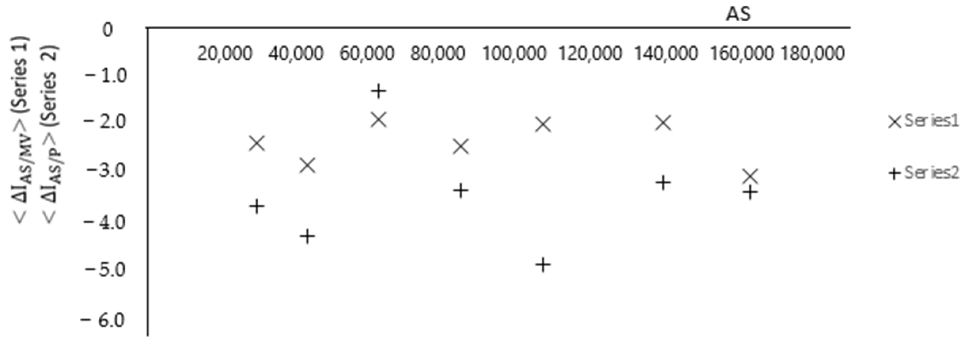
| Commune | λ (bits/h) | Dc | Sk (bits/h) | H | LZ | Τ = 1/SK (h) | |
|---|---|---|---|---|---|---|---|
| Las Condes (LC) | |||||||
| X | 0.238 ± 0.015 | 2.099 ± 0.135 | 0.611 | 0.902570 | 0.10850 | 1.636 | −0.791 |
| Y | 0.325 ± 0.026 | 3.098 ± 0.899 | 0.296 | 0.754360 | 0.09634 | 3.378 | −1.079 |
| Z | 0.168 ± 0.013 | 3.852 ± 0.200 | 0.437 | 0.876525 | 0.47844 | 2.288 | −0.558 |
| SK, MV = 1.344 | 0.844485 | 0.22776 | ₸ = 2.434 | −2.428 | |||
| W | 0.179 ± 0.015 | 3.916 ± 0.238 | 0.477 | 0.871804 | 0.60284 | 2.096 | −0.595 |
| U | 0.327 ± 0.021 | 4.369 ± 0.152 | 0.368 | 0.851004 | 0.61219 | 2.717 | −1.086 |
| V | 0.499 ± 0.024 | 4.314 ± 0.133 | 0.398 | 0.871258 | 0.65148 | 2.513 | −1.657 |
| SK, P = 1.243 | 0.864688 | 0.62217 | ₸ = 2.442 | −3.338 | |||
| Santiago (SANT) | |||||||
| X | 0.170 ± 0.013 | 4.024 ± 0.339 | 0.385 | 0.904362 | 0.36666 | 2.597 | −0.565 |
| Y | 0.231 ± 0.020 | 1.575 ± 0.465 | 0.266 | 0.755542 | 0.08091 | 3.759 | −0.767 |
| Z | 0.177 ± 0.013 | 4.078 ± 0.327 | 0.403 | 0.878623 | 0.51258 | 2.481 | −0.588 |
| SK, MV = 1.054 | 0.846175 | 0.32005 | ₸ = 2.946 | −1.920 | |||
| W | 0.248 ± 0.016 | 4.001 ± 0.277 | 0.447 | 0.876730 | 0.55280 | 2.096 | −0.824 |
| U | 0.375 ± 0.022 | 3.672 ± 0.345 | 0.278 | 0.844136 | 0.48218 | 3.597 | −1.246 |
| V | 0.336 ± 0.024 | 3.278 ± 0.156 | 0.106 | 0.936006 | 0.52988 | 9.434 | −1.116 |
| SK, P = 0.831 | 0.885624 | 0.52162 | ₸ = 5.042 | −3.186 | |||
| Independencia (IND) | |||||||
| X | 0.222 ± 0.015 | 2.093 ± 0.148 | 0.543 | 0.902606 | 0.10710 | 1.842 | −0.737 |
| Y | 0.353 ± 0.022 | 2.581 ± 0.881 | 0.308 | 0.812761 | 0.07249 | 3.246 | −1.173 |
| Z | 0.133 ± 0.012 | 3.927 ± 0.235 | 0.436 | 0.891302 | 0.49808 | 2.294 | −0.442 |
| SK, MV = 1.287 | 0.868889 | 0.22589 | ₸ = 2.461 | −2.352 | |||
| W | 0.209 ± 0.014 | 3.755 ± 0.236 | 0.498 | 0.886482 | 0.60237 | 2.008 | −0.694 |
| U | 0.307 ± 0.018 | 4.252 ± 0.154 | 0.506 | 0.884166 | 0.58367 | 1.976 | −1.019 |
| V | 0.585 ± 0.025 | 3.824 ± 0.211 | 0.365 | 0.898487 | 0.60845 | 2.739 | −1.943 |
| SK, P = 1.369 | 0.889712 | 0.59816 | ₸ = 2.241 | −3.656 | |||
| La Florida (LF) | |||||||
| X | 0.166 ± 0.012 | 4.116 ± 0.286 | 0.364 | 0.910665 | 0.35123 | 2.747 | −0.551 |
| Y | 0.214 ± 0.020 | 1.374 ± 0.789 | 0.293 | 0.771460 | 0.08278 | 3.413 | −0.711 |
| Z | 0.208 ± 0.014 | 4.449 ± 0.344 | 0.473 | 0.883141 | 0.50182 | 2.114 | −0.691 |
| SK, MV = 1.130 | 0.855088 | 0.31194 | ₸ = 2.758 | −1.953 | |||
| W | 0.295 ± 0.016 | 4.055 ± 0.300 | 0.448 | 0.873495 | 0.56215 | 2.232 | −0.980 |
| U | 0.375 ± 0.022 | 4.073 ± 0.275 | 0.341 | 0.850949 | 0.50510 | 2.933 | −1.246 |
| V | 0.792 ± 0.029 | 3.694 ± 0.405 | 0.357 | 0.916451 | 0.57852 | 2.655 | −2.631 |
| SK, P = 1.146 | 0.880298 | 0.54859 | ₸ = 2.760 | −4.857 | |||
| Puente Alto (PA) | |||||||
| X | 0.130 ± 0.012 | 3.120 ± 0.234 | 0.419 | 0.905320 | 0.38537 | 2.386 | −0.432 |
| Y | 0.607 ± 0.025 | 1.403 ± 0.572 | 0.293 | 0.793516 | 0.08605 | 3.413 | −2.016 |
| Z | 0.181 ± 0.013 | 3.852 ± 0.228 | 0.374 | 0.891406 | 0.43354 | 2.674 | −0.601 |
| SK, MV = 1.086 | 0.863414 | 0.30165 | ₸ = 2.824 | −3.049 | |||
| W | 0.276 ± 0.016 | 4.406 ± 0.320 | 0.501 | 0.878464 | 0.50977 | 1.996 | −0.917 |
| U | 0.415 ± 0.024 | 2.446 ± 0.650 | 0.072 | 0.868495 | 0.37882 | 13.888 | −1.378 |
| V | 0.327 ± 0.024 | 2.403 ± 0.347 | 0.306 | 0.852885 | 0.54906 | 3.268 | −1.086 |
| SK, P = 0.879 | 0.866615 | 0.47922 | ₸ = 6.384 | −3.359 | |||
| El Bosque (EB) | |||||||
| X | 0.231 ± 0.015 | 2.713 ± 0.111 | 0.608 | 0.908657 | 0.10616 | 1.645 | −0.767 |
| Y | 0.424 ± 0.024 | 2.764 ± 0.906 | 0.355 | 0.820853 | 0.07717 | 2.817 | −1.408 |
| Z | 0.192 ± 0.014 | 3.941 ± 0.249 | 0.437 | 0.887640 | 0.48171 | 2.288 | −0.638 |
| SK, MV = 1.400 | 0.872383 | 0.22168 | ₸ = 2.250 | −2.813 | |||
| W | 0.251 ± 0.016 | 3.601 ± 0.128 | 0.520 | 0.883469 | 0.61687 | 1.923 | −0.833 |
| U | 0.319 ± 0.018 | 4.338 ± 0.178 | 0.537 | 0.872094 | 0.59068 | 1.862 | −1.060 |
| V | 0.722 ± 0.028 | 4.360 ± 0.166 | 0.432 | 0.921180 | 0.60050 | 2.315 | −2.398 |
| SK, P = 1.489 | 0.892248 | 0.60268 | ₸ = 2.033 | −4.291 | |||
| Pudahuel (P) | |||||||
| X | 0.242 ± 0.015 | 3.021 ± 0.181 | 0.242 | 0.908026 | 0.38256 | 4.132 | −0.804 |
| Y | 0.143 ± 0.017 | 1.876 ± 0.571 | 0.230 | 0.737256 | 0.08325 | 4.347 | −0.475 |
| Z | 0.174 ± 0.013 | 4.204 ± 0.372 | 0.398 | 0.891302 | 0.49808 | 2.513 | −0.578 |
| SK, MV = 0.870 | 0.845528 | 0.32130 | ₸ = 3.664 | −1.857 | |||
| W | 0.280 ± 0.016 | 3.967 ± 0.271 | 0.459 | 0.885674 | 0.56262 | 2.179 | −0.930 |
| U | 0.386 ± 0.021 | 3.746 ± 0.189 | 0.346 | 0.860764 | 0.55841 | 2.890 | −1.282 |
| V | 0.731 ± 0.028 | 3.795 ± 0.138 | 0.367 | 0.912855 | 0.58086 | 2.725 | −2.428 |
| SK, P = 1.172 | 0.886431 | 0.56730 | ₸ = 2.598 | −4.640 | |||
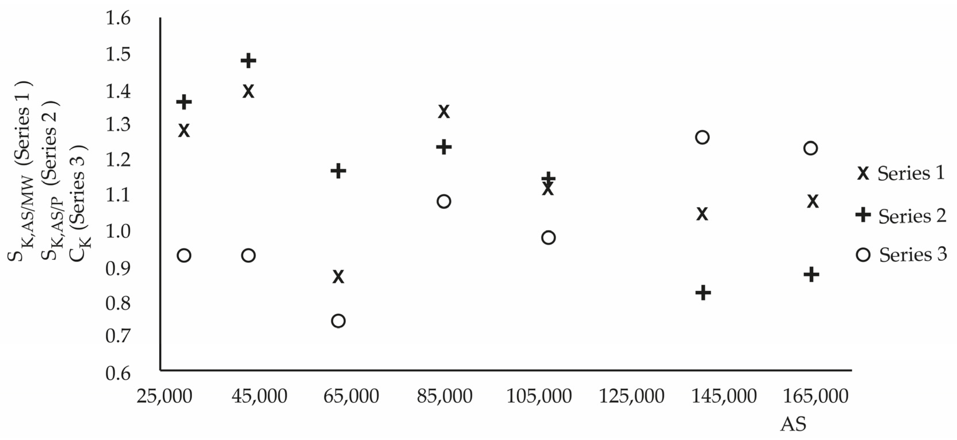
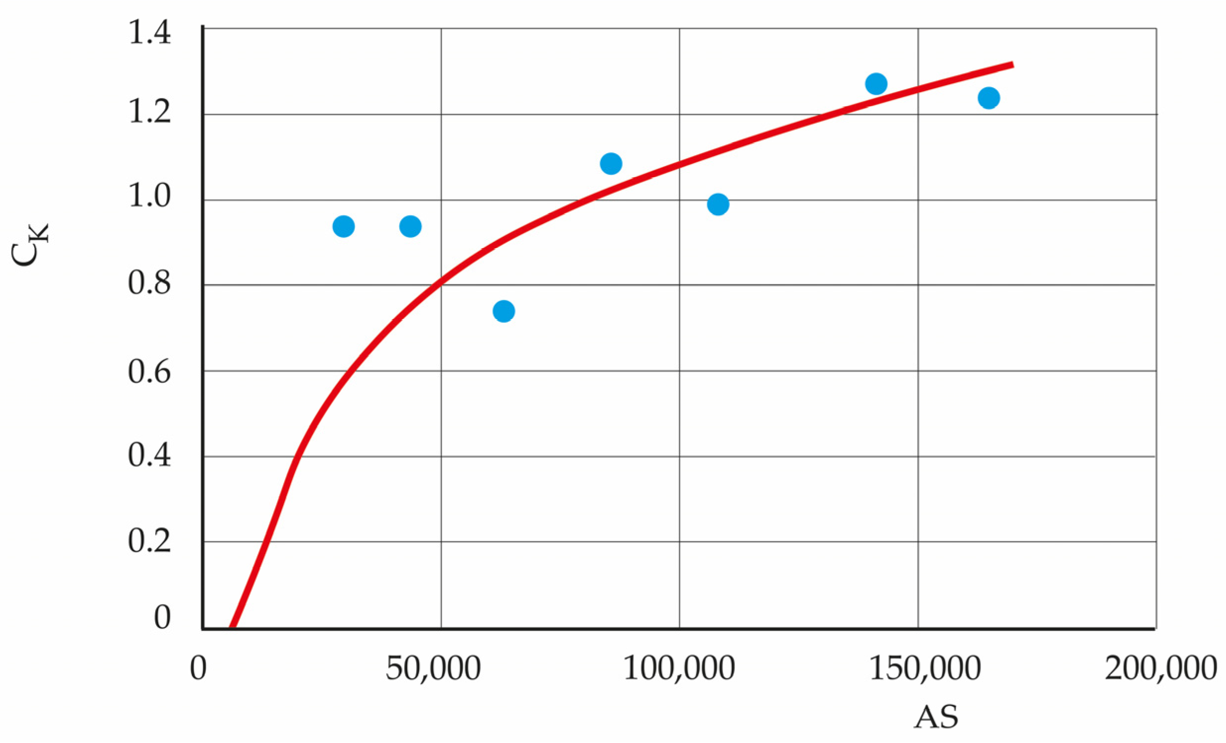
| Commune | AS | SK, AS/MV | SKAS/,P | CK = SK, AS/MV/SK, AS/P |
|---|---|---|---|---|
| La Florida (EML) | 108,264 | 1.130 | 1.146 | 0.986 |
| Las Condes (EMM) | 85,890 | 1.344 | 1.243 | 1.081 |
| Santiago (EMN) | 141,401 | 1.054 | 0.831 | 1.268 |
| Pudahuel (EMO) | 63,290 | 0.870 | 1.172 | 0.742 |
| Puente Alto (EMS) | 165,038 | 1.086 | 0.879 | 1.235 |
| El Bosque (EMQ) | 43,638 | 1.400 | 1.489 | 0.940 |
| Independencia (EMF) | 29,960 | 1.287 | 1.369 | 0.940 |
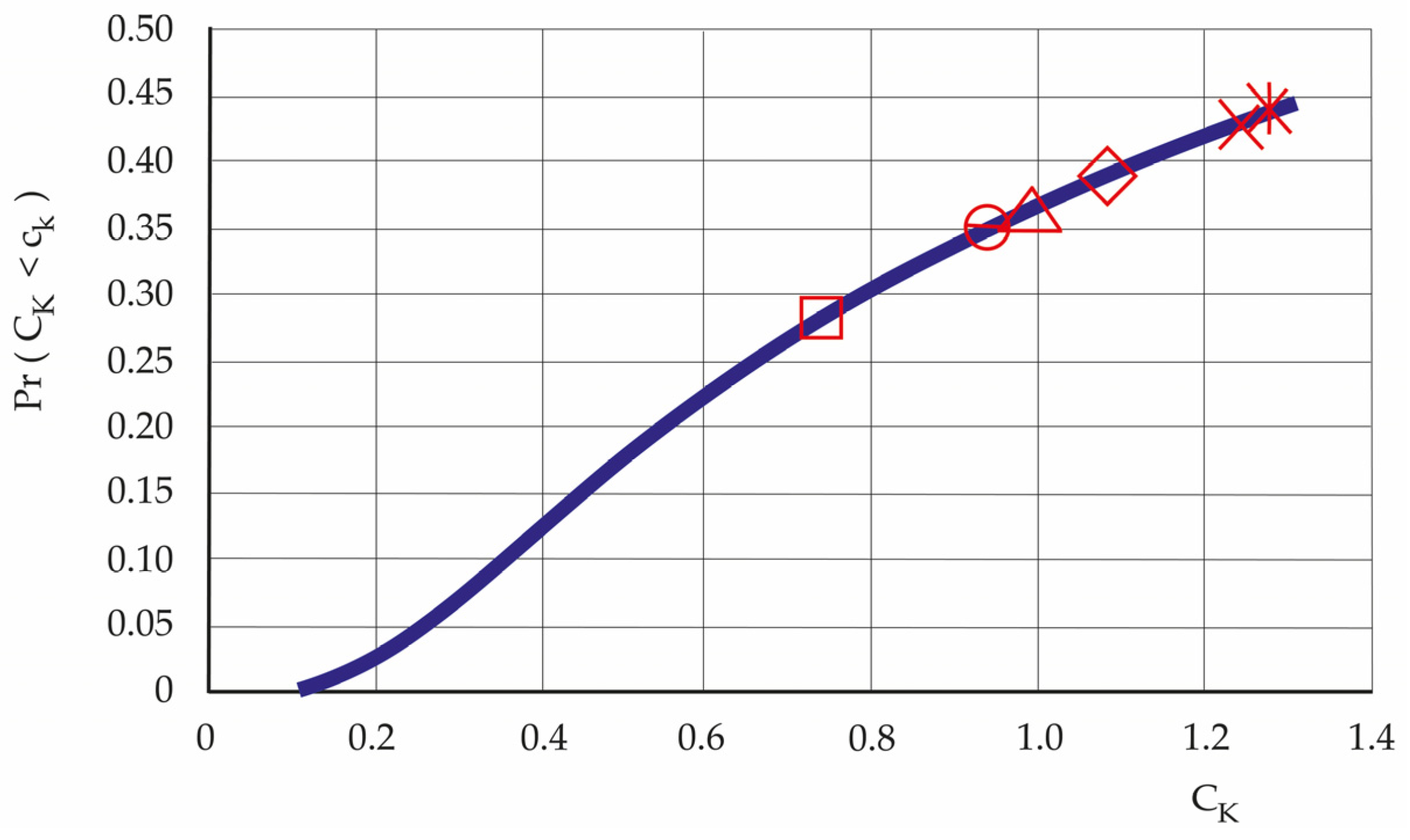
| Localization | AS (31 March 2020–9 January 2023) | CK (2020–2023) | Pr | Diffusion Type |
|---|---|---|---|---|
| EMO | 63,290 | 0.74 | 0.28 | sub diffusion |
| EMQ | 43,638 | 0.94 | 0.35 | sub diffusion |
| EMF | 29,960 | 0.94 | 0.35 | sub diffusion |
| EML | 108,264 | 0.99 | 0.37 | diffusion |
| EMM | 85,890 | 1.08 | 0.39 | super-diffusion |
| EMS | 165,038 | 1.24 | 0.43 | super-diffusion |
| EMN | 141,401 | 1.27 | 0.44 | super-diffusion |
| EML | EMM | EMV | EMN | EMS | EMO | Average by Commune | |
|---|---|---|---|---|---|---|---|
| 2010–2013 | |||||||
| (°C) | 15.4 | 15.86 | 15.80 | 15.34 | 14.70 | 16.80 | 15.65 |
| (%) | 58.20 | 58.13 | 57.34 | 60.22 | 60.07 | 57.52 | 58.58 |
| 2017–2020 | |||||||
| (°C) | 16.12 | 15.57 | 16.85 | 16.17 | 15.53 | 16.78 | 16.17 |
| (%) | 55.31 | 55.00 | 58.95 | 57.31 | 56.07 | 59.22 | 56.98 |
| 2019–2022 | |||||||
| (°C) | 16.10 | 14.70 | 15.50 | 16.05 | 15.42 | 15.31 | 15.51 |
| (%) | 56.20 | 57.83 | 61.20 | 60.84 | 56.96 | 61.32 | 59.10 |
| Actors | Human Activities | Check | Effects |
|---|---|---|---|
| population | mandatory use of a mask, confinement of the population to their homes, vaccination process of the population (two and three doses), increase in hospital beds and equipment, orders for essential goods delivered to homes, attention in commerce (supermarkets, etc.) by small groups of people, street signs to maintain distances among people | Ministry of Health, police from Chilean Companies | deserted streets, irruption of wildlife in the city, crime reduction |
| culture and information | improvement in personal hygiene, development of a culture of hygiene in public and private facilities, permanent information on the pandemic through the media, companies, educational establishments, etc. | Ministry of Health, Ministry of Education, Media | learning |
| travels | mobility passes for people with full doses of vaccines, reduced travel by air, land, and sea except for very justified cases, police and military control of routes, mobility passes requested at police stations | SINCA, measurements, police from Chile | entropy calculation, control of the population |
| teaching and work | teaching via the internet, work via the internet, financial aid vouchers for workers, pension fund withdrawals, boxes with food and toiletries | educational centers closed, companies with no or very little activity, Congress, SINCA | low quality of learning, disorders psychological, overweight |
| wildlife | lockdown of the population in their homes | Media, population, wildlife organizations | irruption of wild fauna in cities |
Disclaimer/Publisher’s Note: The statements, opinions and data contained in all publications are solely those of the individual author(s) and contributor(s) and not of MDPI and/or the editor(s). MDPI and/or the editor(s) disclaim responsibility for any injury to people or property resulting from any ideas, methods, instructions or products referred to in the content. |
© 2024 by the authors. Licensee MDPI, Basel, Switzerland. This article is an open access article distributed under the terms and conditions of the Creative Commons Attribution (CC BY) license (https://creativecommons.org/licenses/by/4.0/).
Share and Cite
Pacheco, P.; Mera, E.; Navarro, G. The Effects of Lockdown, Urban Meteorology, Pollutants, and Anomalous Diffusion on the SARS-CoV-2 Pandemic in Santiago de Chile. Atmosphere 2024, 15, 414. https://doi.org/10.3390/atmos15040414
Pacheco P, Mera E, Navarro G. The Effects of Lockdown, Urban Meteorology, Pollutants, and Anomalous Diffusion on the SARS-CoV-2 Pandemic in Santiago de Chile. Atmosphere. 2024; 15(4):414. https://doi.org/10.3390/atmos15040414
Chicago/Turabian StylePacheco, Patricio, Eduardo Mera, and Gustavo Navarro. 2024. "The Effects of Lockdown, Urban Meteorology, Pollutants, and Anomalous Diffusion on the SARS-CoV-2 Pandemic in Santiago de Chile" Atmosphere 15, no. 4: 414. https://doi.org/10.3390/atmos15040414
APA StylePacheco, P., Mera, E., & Navarro, G. (2024). The Effects of Lockdown, Urban Meteorology, Pollutants, and Anomalous Diffusion on the SARS-CoV-2 Pandemic in Santiago de Chile. Atmosphere, 15(4), 414. https://doi.org/10.3390/atmos15040414