Assessment of Water Resources under Climate Change in Western Hindukush Region: A Case Study of the Upper Kabul River Basin

Abstract

This study aims to estimate the surface runoff and examine the impact of climate change on water resources in the Upper Kabul River Basin (UKRB). A hydrological model was developed using the Soil and Water Assessment Tool (SWAT) from 2009 to 2019. The monthly calibration was conducted on streamflow in six stations for the period from 2010 to 2016, and the results were validated from 2017 to 2018 based on available observed data. The hydrological sensitivity parameters were further prioritized using SWAT-CUP. The uncertainty of the model was analyzed by the 95% Prediction Uncertainty (95PPU). Future projections were analyzed for the 2040s (2030–2049) and 2090s (2080–2099) compared to the baseline period (1986–2005) under two representation concentration pathways (RCP4.5, RCP8.5). Four Regional Climate Models (RCMs) were bias-corrected using the linear scaling bias correction method. The modeling results exhibited a very reasonable fit between the estimated and observed runoff in different stations, with NS values ranging from 0.54 to 0.91 in the calibration period. The future mean annual surface runoff exhibited an increase in the 2040s and 2090s compared to the baseline under both RCPs of 4.5 and 8.5 due to an increase in annual precipitation. The annual precipitation is projected to increase by 5% in the 2040s, 1% in the 2090s under RCP4.5, and by 9% in the 2040s and 2% in the 2090s under RCP8.5. The future temperature is also projected to increase and consequently lead to earlier snowmelt, resulting in a shift in the seasonal runoff peak to earlier months in the UKRB. However, the shifts in the timing of runoff could lead to significant impacts on water availability and exacerbate the water stress in this region, decreasing in summer runoff and increasing in the winter and spring runoffs. The future annual evapotranspiration is projected to increase under both scenarios; however, decreases in annual snowfall, snowmelt, sublimation, and groundwater recharge are predicted in the UKRB.

1. Introduction

During the last two decades of the 21st century, global mean temperature increases of 0.99 °C (2001–2020) and 1.09 °C (2011–2020) were observed compared to 1850–1900, with larger increases over lands (1.59 °C) compared to the oceans (0.88 °C) [1,2]. Climate change is increasingly acknowledged as the greatest global issue, exerting significant impacts on hydrological processes, including precipitation, evapotranspiration, runoff, and total water availability [3]. Consequently, these changes create significant challenges to the sustainability of water resources, the environment, and human and animal lives worldwide [4]. Additionally, the melting of snow and glaciers can be impacted by global climate change, altering the timing and amount of runoff in mountainous areas [5]. In Asia, the Hindu Kush-Himalaya (HKH) region has the highest density of glaciers outside the poles and feeds many larger rivers [6]. The HKH region is expected to see higher rates of mean surface temperature rise towards 2100 than the global average [7,8]. With increasing temperature and changes in precipitation, river flow will be significantly affected and alter the water cycle in this region [7], including the Kabul River, which is one of the major tributaries of the Indus River Basin.

Afghanistan is categorized as a semi-arid to arid climate and is highly vulnerable to climate change, with annual precipitation ranging from 200 to 500 mm. The country has repeatedly experienced prolonged drought [3,9,10]. The annual precipitation hardly satisfies the incremental water demand of the whole country, although precipitation varies geographically [11]. The snow and glaciers in Afghanistan are at high risk due to climate change, especially in the summer; the snow and glacier cover is in retreat [5] due to high melting. Winter precipitation accounts for 80% of the country’s total water resources; however, it is not enough to satisfy the crop’s water demand in the summer [12]. Likewise, 85% of Afghanistan’s total agricultural yield is produced by irrigation, which consumes 98% of the water consumption. However, irrigation performance at the basin level is poor [12,13]. Any change or deficit in the water availability due to climate change can severely impact the people whose livelihoods depend on agriculture in Afghanistan.

The Kabul River Basin (KBR), one of Afghanistan’s five river basins, has transboundary water resources that flow into Pakistan [3,14]. The KRB covers more than 12% of the country’s territory and generates approximately 26% of the country’s total annual streamflow. KRB accounts for 35% of the population and has the fastest population growth rate in the country, which plays a key role in developing the country’s economic growth. Irrigation water availability in the KRB relies on effective rainfall and surface runoff generated by snow and glaciers in the upstream regions [3,15]. It is expected that the precipitation pattern will change due to climate change, with the basin receiving less snow but more rainfall, resulting in the tendency for a quicker response of the basin to rainfall. Consequently, there would be an increased mismatch between water availability and peak demand in KRB. Therefore, to develop a sustainable plan for managing water resources against climate change, preparing for recurring natural hazards (e.g., floods and droughts), and preventing financial losses under climate change, there is a high demand to assess future water availability in this basin. However, there are some studies that have discussed the climate and hydrologic trends in the KRB, including the Afghanistan and Pakistan regions. The studies estimated that river flows will increase in the future due to increased precipitation and enhanced melts [16]. Studies also reported higher rates of warming for the basin than the global average, as warming is projected to increase by 1.8 °C, 3.5 °C, and 4.8 °C for the 2020, 2050, and 2080 periods, respectively, in the KRB [17]. Recently, a study examined the climate change impacts on water resources in the KRB [12] while neglecting the bias correction of the RCM output and uncertainty associated with Global Climate Models (GCMs) by focusing on one RCM. According to Ref. [12], runoff will fall by a maximum of 5% and 8.5% under RCP 4.5 and 8.5 scenarios, respectively, until the end of 2030 in the KRB. Also, Ref. [18] conducted a study to assess the performance of SWAT, evaluate different statistical metrics during calibration and validation, and analyze the impacts of climate change on streamflow from 2020 to 2045 in the Alingar Watershed of the KRB. The results from Ref. [18] showed that the mean annual streamflow will see a decline of 15.2% to 15.6% by 2045 under RCP 4.5 and 8.5 scenarios in the Alingar watershed. However, uncertainty in their results was larger due to lacking bias corrections of RCMs and using only one RCM (RegCM4). Additionally, temperature and precipitation are very significant weather elements with a significant impact on hydrology. Therefore, the bias correction of temperature and precipitation in the RCMs is essential before applying any climate change or hydrology study.

However, previous studies show there is less/a lack of hydrological modeling in future runoff estimation, snow changes, and total water availability under climate change using the bias-corrected data in KRB, especially in the upper three mountainous watersheds selected in this study (e.g., Kabul, Logar, and Ghorband and Panjshir watersheds).

Therefore, the main objective of this study is to (a) build, calibrate, and validate the SWAT hydrological model for the current 2009–2019 period, (b) perform bias correction in RCMs’ output and incorporate them into the SWAT model, and (c) estimate and analyze the future monthly, seasonal and annual runoff and total water availability under climate change in the Upper Kabul River Basin (UKRB). The climate variables were generated using the mean ensemble of four bias-corrected CORDEX-CMIP5-RCMs to estimate runoff for the historical (1986–2005) and two future time periods: the 2040s (2030–2049) and 2090s (2080–2099). The Soil and Water Assessment Tool (SWAT) hydrologic model and two representation concentration pathways (RCP4.5 and RCP8.5) were implemented. The findings of this research are crucial in formulating effective water management strategies for future water availability and conducting demand analyses. In particular, the insights obtained will be beneficial for water-scarce cities like Kabul city, enabling them to tackle challenges associated with water shortages and drought conditions in the future.

Study Area

The UKRB is located within the latitude range of 33.6° to 35.9° north, the longitude range of 67.63° to 70.30° east, and an altitude ranging from 995 m to 5694 m above sea level (Figure 1). The northern and northeastern part of the basin is located in the highlands of the Hindukush Mountains, which are drained by the Ghorband and Panjshir rivers and are the main source of water for the KRB. The Kabul River originates from the Paghman mountain on the west and Koh-e-Safi Mountain on the east. The UKRB includes three main river systems, the Ghorband and Panjshir River, the Logar River and the Kabul River. The climate is characterized by cold winters and hot summers with less or no precipitation and stream flow, except for the rivers and streams fed by melting snow or glaciers [19]. The precipitation and temperature vary significantly in the basin due to elevation variations in different seasons. The period from June to August experiences the highest temperatures in the UKRB, with July being the warmest month, reaching a monthly mean of 25 °C. On the other hand, the coldest months occur from November to February, with January being the chilliest, with a monthly mean of −11 °C. These temperature patterns were observed from 1986 to 2005. Based on rainfall data from the APHRODITE database spanning a 20-year period (1986–2005), the average annual precipitation in the UKRB is approximately 420 mm. In the northern parts of the KRB, there are high mountains and steep slopes, while the southern portions are dominated by low mountain ranges, foothills, and plains. The primary flow contributions from the northern tributaries are due to snowmelt and glacier meltwater. Glaciers serve as a long-term asset in high mountains by stabilizing the water supply within and between years. They play a critical role in ensuring consistent stream flows in the rivers.

2. Materials and Methods

The materials and methods used in this study are explained in the following subsections.

2.1. Spatial Data (Topographic, Land Use, Soil)

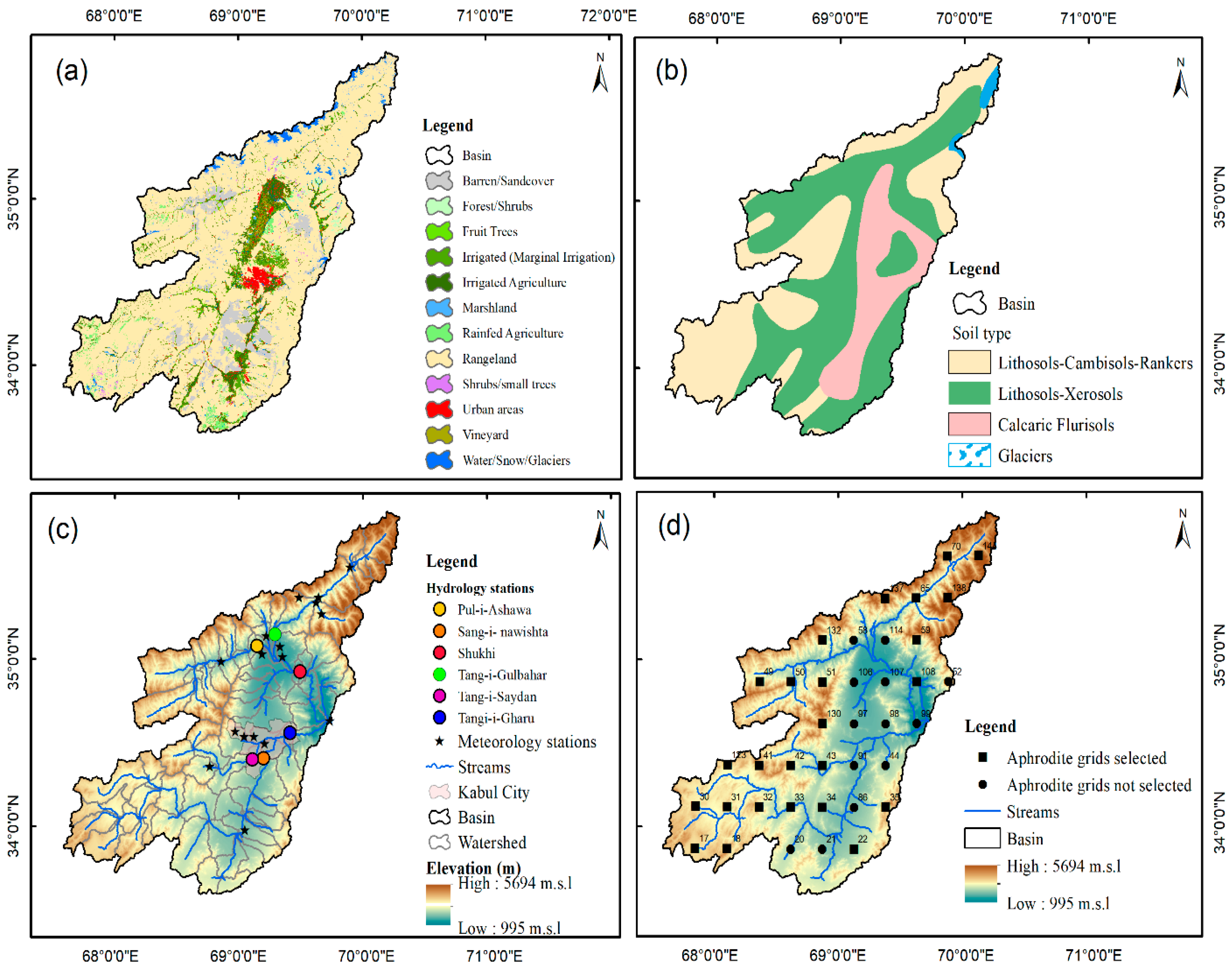
The sub-basin delineation of the UKRB was conducted using the Digital Elevation Model (DEM) from the Shuttle Radar Topographic Mission-(SRTM) with a 30 m × 30 m resolution. The DEM was obtained from the U.S. Geological Survey’s Earth Explorer database “https://earthexplorer.usgs.gov (accessed on 25 January 2020)”. The land use data were obtained from the Landcover Atlas of the Islamic Republic of Afghanistan, which was published by the Ministry of Agriculture, Irrigation and Livestock [20]. The land use map was re-classified into thirteen major classes based on SWAT input requirements (Figure 2). The area of different land use classes is shown in Supplementary Table S1. Soil information was derived from the FAO-soil map of the world “https://www.fao.org/soils-portal/soil-survey/soil-maps-and-databases/faounesco-soil-map-of-the-world/en/ (accessed on 2 May 2020)”. The soil texture in the UKRB is predominantly loam, and it has a hydrologic soil group of C and D. The hydrological soil group refers to the Natural Resource Conservation Service (NRCS) soil classification based on the infiltration characteristics of the soil (Figure 2). The area of soil classification is shown in Supplementary Table S2.

2.2. Weather Data (Current Scenario)

The daily precipitation, maximum temperature (Tmax), and minimum temperature (Tmin) for the period from 1 January 2009 to 31 December 2019 were collected from 21 meteorological stations located within the KRB in Afghanistan (Figure 2c). Among these meteorological stations, the daily precipitation and temperature data of 13 stations were obtained from the National Water Affairs Regulation Authority (NAWARA), while only the daily precipitation of 8 stations was obtained from the Ministry of Agriculture, Irrigation and Livestock (MAIL) in Afghanistan. Moreover, daily observed discharge data from 1 January 2010 to 31 September 2018 were obtained from NAWARA. These data were collected from six hydrological stations installed on different rivers and tributaries in the KRB and were used for the calibration and validation of the SWAT model. The details of meteoritical and hydrological stations are shown in Supplementary Tables S3 and S4. The sources of all data used for building the SWAT model are shown in Supplementary Table S5.

2.3. Regional Climate Models (RCMs)

The daily temperature and precipitation data for the baseline and future projections were obtained from the Coordinated Regional Downscaling Experiment (CORDEX) South Asia Domain, along with their corresponding CMIP5-driving RCMs. These datasets are hosted by the German Climate Computing Centre (DKRZ) and were accessed from “https://esgf-data.dkrz.de/search/cmip5-dkrz/ (accessed on 10 March 2021)”. CORDEX focuses on the high-resolution climate information produced by different dynamical and statistical downscaling techniques, and it aims to provide coordinated sets of high-resolution regional climate projections worldwide. Four climate models, including two RCPs, 4.5 and 8.5, were selected in this study (

Table 1. Description of regional climate models selected for this study. RCPs are RCP4.5 and RCP8.5.

Domain	RCMs	Driving GCMs	Historical Data	RCPs	Institution	Resolution
WAS-44	RCA4	CanESM2-CCCma	1951–2005	2006–2100	SMHI 2	0.44° × 0.44°
WAS-44	RegCM4-4	NOAA-GFDL-ESM2M	1951–2005	2006–2099	IITM 3	0.44° × 0.44°
WAS-44i	REMO2009	MPI-ESM-LR	1961–2005	2006–2100	MPI-CSC 4	0.44° × 0.44°
WAS-44	RCA4	MIROC5	1961–2005	2006–2100	SMHI 2	0.44° × 0.44°

Note: WAS stands for the South Asia domain; 44 is the grid resolution, and the suffix i stands for the mean regular grid; SMHI: Swedish Meteorological and Hydrological Institute, Rossby Centre (Sweden); IITM: Indian Institute of Tropical Meteorology (India); and MPI-CSC: Max Planck Institute for Meteorology—Climate Service Center at Germany. The data of 1986–2005, 2030–2049 (2040s), and 2080–2099 (2090s) were used for the historical and future time periods, respectively.

). The RCMs were selected based on data availability for Afghanistan and the previous studies [19,21,22].

2.4. Bias Correction Procedure

Despite the finer grid resolution of RCMs compared to GCMs, they are still not directly suitable to use for regional hydrologic impact studies. Therefore, in the case of the historical data availability of the ground station, bias corrections of the RCMs based on ground data are necessary. According to Ref. [23], the simulation of temperature and precipitation data often exhibits significant biases due to systematic model errors, discretization, and spatial averaging within the grid cells in the RCMs, which hinder the use of simulated climate data as a direct input for hydrological modeling and climate change studies. To address this issue, the linear scaling bias correction method is employed to minimize the discrepancies between RCM’s precipitation and temperature with the APHRODITE data. Due to the lack of observed historical data in the study area, APHRODITE data were selected as observations and used during the bias correction of the RCMs. The Climatic Model data for the hydrologic modeling (CMhyd) tool [24] were used for the bias correction procedure. The linear scaling method used in this study is based on Ref. [23] and expressed by Equations (1)–(4).

$$P_{Cont}^{\mathrm{\ast }}\left(i\right)=P_{raw}\left(i\right)\times \left[\frac{{\mathrm{\mu }}_m\left(P_{obs}\left(i\right)\right)}{{\mathrm{\mu }}_m\left(P_{raw}\left(i\right)\right)}\right]$$

(1)

$$P_{Scen}^{\ast }\left(i\right)=P_{raw}\left(i\right)\times \left[\frac{{\mu }_m\left(P_{obs}\left(i\right)\right)}{{\mu }_m\left(P_{raw}\left(i\right)\right)}\right]$$

(2)

$$T_{Cont}^{\ast }\left(i\right)=T_{raw}\left(i\right)+{\mathrm{\mu }}_m\left(T_{obs}\left(i\right)\right)-{\mathrm{\mu }}_m\left(T_{raw}\left(i\right)\right)$$

(3)

$$T_{Scen}^{\ast }\left(i\right)=T_{raw}\left(i\right)+{\mathrm{\mu }}_m\left(T_{obs}\left(i\right)\right)-{\mathrm{\mu }}_m\left(T_{raw}\left(i\right)\right)$$

(4)

where P* and T* represents the final bias-corrected precipitation and temperature, _Cont and _Scen represent the control (historical) and future periods, and P_raw and T_raw are the raw precipitation and temperature from RCMs, respectively. (i) is the time interval (daily), P_obs and T_obs represent the observed precipitation and temperature, and µm represents the mean values for the month.

2.5. Hydrological Model

The Soil and Water Assessment Tool (SWAT) [25,26,27] is utilized to estimate the streamflow, analyze hydrologic processes, and predict the impacts of climate change on surface runoff in the UKRB. SWAT is a process-based, spatially distributed, and time-continuous model that operates by spatially dividing a basin into multiple sub-basins using the topography of the area. Each sub-basin is further discretized into Hydrologic Response Units (HRUs). During the model setup, the initial step involved watershed delineation. Subsequently, three preprocessed spatial datasets (slope, land use, and soil data) were employed to determine the HRUs once the watershed delineation was completed. By utilizing the HRUs as a basis, it became possible to determine all the components of the water balance for lands that shared similar topography, land use, and soil. This assumption was based on the notion that lands with similar characteristics would exhibit similar hydrologic behaviors [28,29,30].

Subsequently, the model was fed with climatic data, which included daily precipitation, minimum temperature, and maximum temperature. To address data gaps in some meteorology stations, the Inverse Distance Interpolation method (IDW) was employed to fill the missing values. The runoff generation method was set to be estimated using the Soil Conservation Curve Number (SCS-CN) method, while the potential evapotranspiration was estimated using the Hargreaves Equation (5) [31]. Channel water routing was conducted using the variable storage method, while the simulation of rainfall distribution employed the mixed exponential method in the SWAT.

$$\lambda E_0=0.0023 ·{ H}_{0 }·{\left(T_{mx}-T_{mn}\right)}^{0.5} · \left({\stackrel{-}{T}}_{av}+17.8\right)$$

(5)

where $\lambda$ is the latent heat of vaporization (MJ Kg⁻¹), $E_0$ is potential evapotranspiration (mm/day), $H_{0 }$is the extra-terrestrial radiation (MJ/m. day), T_mx is the maximum air temperature for a given day (°C), T_mn is the minimum air temperature for a given day (°C), and ${\stackrel{-}{T}}_{av}$ is the mean air temperature for a given day (°C).

During winter, the KRB experiences significant snowfall, which accumulates and remains stored in high altitudes of the mountains. In the summer, the rivers experience snowmelt from the mountains. Therefore, the snowmelt process was considered during the calibration and validation of the SWAT model in this study. The SWAT model uses a temperature-index-based method to estimate the snowmelt process. The model considers snowmelt as rainfall to calculate runoff and seepage. The snowmelt is estimated as a linear function of the difference between the average snowpack temperature and maximum air temperature on a given day and the base or threshold temperature [32]. Equation (6) outlines the calculation of snowmelt in the SWAT model.

$${\mathit{SNO}}_{mlt}=b_{mlt}\times {\mathit{sno}}_{cov}\times \frac{T_{snow}+T_{mx}}{2}-T_{mlt}$$

(6)

where SNO_mlt is the amount of snowmelt per day (mm H₂O), b_mlt is the melt factor (mm H₂O/[day·°C]), sno_cov is the fraction of the HRU’s area covered by snow, T_snow is the snowpack temperature on a given day (°C), T_mx is the maximum air temperature on a given day (°C), and T_mlt is the base temperature above which snowmelt is allowed (°C). The model incorporates the leap year in its calculations automatically. The melt factor allows for seasonal variations, with maximum and minimum values occurring in summer and winter, respectively, and is calculated as Equation (7).

$$b_{mlt}=\frac{b_{mlt6}+b_{mlt12}}{2}+\frac{b_{mlt6}-b_{mlt12}}{2}Sin\left[\frac{2\pi }{365}.\left(d_n-81\right)\right]$$

(7)

where b_mlt is the melt factor (mm H₂O/[day·°C]), b_mlt6 is the melt factor for 21st June (mm H₂O/[day·°C]), b_mlt12 is the melt factor for 21st December (mm H₂O/[day·°C]), and d_n is the number of days in the year, 365 [7,27]. Once all the processes were completed, the SWAT simulation was initiated. The model was configured to run continuously from January 2009 to December 2019, with the first year (2009) selected as the warm-up period. Following the calibration and validation of the model, the bias-corrected precipitation and temperature from the RCMs’ output were employed to examine the effects of climate change on runoff in the UKRB. The methodology used in this study is summarized in Figure 3.

2.6. Calibration and Validation

The successful application of hydrologic models is highly dependent on the calibration, validation, and sensitivity analysis [33]. Two procedures, (1) the manual calibration helper in SWAT and (2) the automatic calibration approach of Sequential Uncertainty Fitting Version-2 (Sufi-2) in SWAT-CUP, were applied for model calibration [33,34]. Sufi-2 is one of the stochastic calibration programs in SWAT-CUP and is a semi-automated inverse modeling procedure based on Latin Hypercube Sampling. A detailed description of SUFI-2 can be found in [30,33,34]. In this study, monthly calibration was conducted on streamflow data in six stations for the period from 2010 to 2016, spanning seven years. The calibration results were then validated using the discharge data from January 2017 to September 2018. The sensitivity analysis was conducted on 27 hydrology-related parameters using the one-at-a-time (OAT) sampling method to assess the impact of each parameter on streamflow. Afterward, the sensitivities of all parameters selected through the OAT method were further prioritized using the global sensitivity analysis option in SWAT-CUP. For the prioritization of sensitive parameters, the p-value and t-state of the global sensitivity procedure were used [33]. Parameters that exhibit smaller p-values and larger t-statistics are considered to be the most sensitive [33]. SUFI-2 operates by performing multiple iterations, with each iteration consisting of several simulations ranging from 300 to 1000. However, if a SWAT project takes too long to run, a reduced number of simulations (200–300) per iteration may be deemed acceptable. In each iteration, the parameter value becomes smaller compared to the previous iteration. As the parameter ranges become smaller, the 95% Prediction Uncertainty (95PPU) envelope also shrinks, leading to smaller P-factor and smaller R-factor values [35]. The model performance indicator for the calibration and validation was carried out using the coefficient of Nash–Sutcliffe Efficiency (NS) [36], Equation (4). The other coefficients, like the coefficient of determination (R²), percent bias (PBIAS) [37], and Kling–Gupta efficiency (KGE) [38], were automatically calculated by the SWAT model using Equations (8)–(11).

$$NS=1-\frac{{\sum }_i{\left(Q_{o,i}-Q_{s,i}\right)}^2}{{\sum }_i{\left(Q_{o,i}-{\overline{Q}}_s\right)}^2}$$

(8)

$$R^2=\frac{{\sum }_i{\left[\left(Q_{o,i}-{\overline{Q}}_o\right)\left(Q_{s,i}-{\overline{Q}}_s\right)\right]}^2}{{\sum }_i{\left(Q_{o,i}-{\overline{Q}}_s\right)}^2 {\sum }_i{\left(Q_{s,i}-{\overline{Q}}_s\right)}^2}$$

(9)

$$PBIAS=\frac{{\sum }_{i=1}^n\left(Q_{o,i}-Q_{s,i}\right)\ast 100}{{\sum }_{i=1}^n\left(Q_{o,i}\right) }$$

(10)

$$KGE=1-\sqrt{{\left(r-1\right)}^2+{\left(\frac{\sigma s}{\sigma o}-1\right)}^2+{\left(\frac{\mu s}{\mu o}-1\right)}^2}$$

(11)

where Q is discharge, $\overline{Q}$ is the mean of discharge, o and s are observed and simulated, i is the ith observed or simulated value, r is the linear scaling correlation between the observed and simulated, $\sigma$ is the standard deviation, and $\mu$ is the mean. Generally, model simulations are considered satisfactory if the NS is greater than 0.50, the R² is greater than 0.60, and the PBIAS is approximately within the range of ±25% [39]. A higher efficiency value indicates a more accurate prediction of the model.

3. Results

3.1. Bias-Corrected Temperature and Precipitation Changes

The precipitation and temperature from 25 grid points of the APHRODITE dataset were selected and used for the bias corrections of the RCMs in the UKRB to analyze the baseline and future changes, Figure 2d. Linear scaling was able to correct the bias more accurately for the precipitation and temperature of the RCMs against the APHRODITE dataset.

Table 2. The future changes in temperature and precipitation in UKRB were compared to the baseline period.

RCP Period	Variable	Spring (MAM)	Summer (JJA)	Autumn (SON)	Winter (DJF)	Annual
RCP4.5 (2040s)	Precipitation	−8%	6%	35%	13%	5%
RCP4.5 (2090s)	Precipitation	−2%	9%	17%	21%	1%
RCP8.5 (2040s)	Precipitation	−12%	18%	0%	12%	9%
RCP8.5 (2090s)	Precipitation	−12%	18%	13%	12%	2%
RCP4.5 (2040s)	Temperature	3.2 °C	1.7 °C	0.2 °C	2.5 °C	+1.9 °C
RCP4.5 (2090s)	Temperature	5.5 °C	2.0 °C	0.1 °C	4.6 °C	+3.1 °C
RCP8.5 (2040s)	Temperature	4.5 °C	3.0 °C	1.4 °C	4.3 °C	+2.4 °C
RCP8.5 (2090s)	Temperature	8.5 °C	4.2 °C	2.4 °C	7.0 °C	+6.1 °C

depicts the future seasonal and annual precipitation and temperature changes compared to the baseline period. The precipitation shows a decrease of −8% and −2% in the spring season compared to the baseline in the 2040s and 2090s, respectively, under RCP4.5. It also shows a drop of −12% in the same season under RCP8.5 for both periods. However, the precipitation shows an increase in the other three seasons compared to the baseline period under both RCPs. The precipitation increases from 6% to 35% in the 2040s and 9% to 21% in the 2090s under RCP4.5, while it shows an increase of 0% to 18% in the 2040s and 12% to 18% in the 2090s under the RCP8.5 scenario. In addition, the mean annual precipitation changes show how, under RCP4.5, there is an increase in annual precipitation of about +5% (21 mm) in the 2040s and an increase of about +1% (3.2 mm) in the 2090s. Moreover, under RCP8.5, the annual precipitation is expected to increase by +9% (37 mm) in the 2040s and about +2% (10 mm) in the 2090s compared to the baseline period.

The monthly temperature shows an overestimation from December to July in both periods under RCP4.5, while in other months, the changes are minimal. Additionally, the monthly temperature shows an increase in all months for the 2040s and 2090s under the RCP8.5 scenario, Figure 4. The monthly temperature peak represents a monthly shift and clearly indicates that June rather than July holds the highest temperature records. Consequently, the future temperature will become warmer in all seasons, especially in spring, summer, and winter seasons. This shift is expected to result in earlier snowmelt in the high mountainous areas and accordingly affect the hydrological regime and the water resources in the study area. The mean annual temperature change shows an increase of +1.9 °C in the 2040s and +3.1 °C in the 2090s under RCP4.5. Likewise, under RCP8.5, the mean annual temperature increases by +2.4 °C in the 2040s and 6 °C in the 2090s, respectively (Table 2).

3.2. Hydrology Results of SWAT (2010–2019)

3.2.1. Model Performance and Sensitivity Analysis

During the calibration of the model, out of the 27 tested parameters, 11 parameters were the most sensitive in the UKRB (

Table 3. The most sensitive parameters that contribute to flow during calibration in the UKRB. v__: existing parameter replaced by a given value; r__: existing parameter multiplied by (1+ a given value).

Parameter	Rank	Details of Abbreviations (Unit)	T-Stat	p-Value	Min Value	Max Value	Fitted Value
v__SOL_AWC.sol	1	Available water capacity of soil (mm·mm−1)	40.99	0.000	0.0	0.2	0.1438
v__GWQMN.gw	2	Threshold depth of water in the shallow aquifer required for return flow to occur (mm·H2O)	7.697	0.000	700.0	900.0	888.33
v__PLAPS.sub	3	Precipitation lapse rate (mm H2O/km)	−7.39	0.000	33.0	100.0	75.321
v__SUB_SMFMX.sno	4	Maximum melt rate for snow during the year (mm H2O °C−1day−1)	−6.88	0.000	0.0	5.0	1.5583
v__ESCO.hru	5	Soil evaporation compensation factor	−2.68	0.008	0.9	1.0	0.9424
v__SUB_TIMP.sno	6	Snowpack temperature lag factor	−2.58	0.014	0.0	1.0	0.8550
v__SMFMN.bsn	8	Minimum melt rate for snow during the year (mm H2O °C−1day−1)	2.53	0.012	0.0	5.0	1.8583
r__CN2.mgt	9	SCS runoff curve number	−2.44	0.015	0.0	0.1	0.0454
v__SUB_SMTMP.sno	10	Snowmelt base temperature (°C)	1.69	0.091	−5.0	5.0	−1.116
v__SUB_SFTMP.sno	11	Snowfall temperature (°C)	1.57	0.115	2.0	4.0	3.9567

). The five most sensitive parameters include SOL_AWC, GWQMN, PLAPS, SMFMX, and ESCO. The sensitive parameters are ranked from top to bottom based on their p-value and t-statistics. The remaining parameters had either very small or no impact on runoff and were, therefore, removed from further iterations. The study area had a total drainage area of about 26,000 km², and its topography differed from mountainous to flat areas with dissimilar climatic conditions. Hence, the precipitation lapse rate (mm H₂O/km) and temperature lapse rate (°C/km) were adjusted by elevation bands in the sub-basins to account for the orographic effects. The orographic climatic effects suggested by money studies in SWAT were considered [31,40].

Figure 5 displays the monthly graphical comparison between the simulated and observed streamflow during the calibration and validation periods. The magnitude of streamflow varies from year to year and is highest between May and August. The streamflow is dominated by peak flows in the summer season due to snow melting in April, followed by June and July each year, and lasts until the end of August. Similar flow peaks can also be seen in the validation graphs. There is an underestimation of the flow peak during calibration for certain years. The simulated baseflow exhibited a very reasonable fit in all stations except for the Pul-i-Ashawa station. In the Pul-i-Ashawa station, the baseflow was slightly overestimated in August and September compared to the observed discharge. This could be due to the uncertainty in the model’s input precipitation and uncertainty in the groundwater-related parameters in the SWAT. According to previous studies, underestimation in hydrological modeling occurs due to observation errors, biases in precipitation, and uncertainties in hydrological modeling [39]. However, the timing of the flow peak is accurate in calibration and validation periods, and the percent bias (PBIAS) remains within an acceptable range. The Nash–Sutcliffe (NS) coefficient values during calibration and validation were 0.91 and 0.93 for Tang-i-Gulbarhar, 0.79 and 0.74 for Shukhi, 0.66 and 0.16 for Pul-i-Ashawa, 0.85 and 0.79 for Tang-i-Gharu, 0.75 and 0.68 Tang-i-Saidan, and 0.54 and 0.21 for Sang-i-Nawishta stations, respectively (

Table 4. The monthly statistical analysis of the calibration and validation results conducted at six stations in UKRB.

Stations	Process	p-Factor	r-Factor	NS	R2	KGE	PBIAS	Conditions
Tang-i-Gulbahar	Calibration	0.87	1.02	0.91	0.92	0.9	4.2	Very good
	Validation	0.57	0.03	0.93	0.95	0.89	−4.8
Pul-i-Ashawa	Calibration	0.79	0.44	0.66	0.67	0.8	2.6	Good
	Validation	0.35	0.2	0.16	0.82	0.27	−36.3
Shukhi	Calibration	0.78	0.3	0.79	0.79	0.82	−3.7	Very good
	Validation	0.39	0	0.74	0.8	0.79	−16.2
Tang-i-Gharu	Calibration	0.52	1.17	0.85	0.89	0.85	1.1	Good
	Validation	0.31	0.1	0.79	0.83	0.71	10.5
Tang-i-Saidan	Calibration	0.58	1.2	0.75	0.78	0.69	22.5	Good
	Validation	0.49	0.3	0.68	0.78	0.77	−13.9
Sang-i-Nawishta	Calibration	0.74	0.22	0.54	0.79	0.35	58.1	Satisfactory
	Validation	0.25	0.01	0.21	0.73	0.02	69.6

). All stations demonstrated good to very good agreements between simulated and observed runoff, except for the Sang-i-Nawishta station, which was satisfactory in this study. The lower NS values at Sang-i-Nawishta could also be due to errors in the observed discharge or input precipitation. The overall range of NS values (Table 4) achieved in this study is aligned with similar studies conducted in larger basins [12,33]. Shukhi station at the Panjshir River recorded the highest annual peak flows in June 2015 and 2016 in the UKRB.

3.2.2. Hydrological Water Balance (2010–2019)

The water balance components are depicted in Figure 6. The monthly total water yield (surface flow + lateral flow + groundwater flow) supplies the river flows with peaks starting in March and continuing until August, with a maximum peak in May. Between February and July, the surface flow contributed more than lateral flow and groundwater flow, with the high peaks of 27 mm in May. This is due to contributions from rainfall and snowmelt. The river flow was mainly supplied by groundwater (baseflow) all through the year, with higher peaks between May and July. Between August to February, the figure clearly shows that the contribution of groundwater flow is greater than surface runoff. This is because, in these months, the occurrence of rainfall and snowfall is minimal, and it may be partly attributed to the melting of snow and glaciers in the UKRB. It can be seen that the water losses due to evapotranspiration (ET) are greater between May and July.

As shown in Figure 6, the inter-annual variation in rainfall was from 287 mm to 544 mm, with minimum rainfall occurring in 2018 and maximum rainfall occurring in 2019. The inter-annual variation in total water yield was from 113.8 mm to 199.5 mm for the same period. This shows that there is some degree of fluctuation in the rainfall and runoff pattern. By inserting an input of 406 mm of annual precipitation, the model estimated 97.5 mm of annual surface runoff and 61.46 mm of annual percolation. Surface runoff accounts for 25%, and groundwater recharge accounts for 12% of the annual hydrological cycle in the UKRB. The ET was estimated at 246.6 mm (63%), which is greater than the total water yield. The soil characteristics of the basin allow a percolation of 61.46 mm, while the return flow contributes 48.66 mm to surface runoff. The re-evaporation (revap) from the shallow aquifer to the root zone was estimated at 9.45 mm, while the lateral streamflow was very small at 0.5 mm in the study area. Moreover, the diagram explaining the annual hydrological model is shown in Supplementary Materials Figure S1.

3.3. Future Hydrological Variation under Predicted Climate Change

3.3.1. Monthly Variations in Streamflow

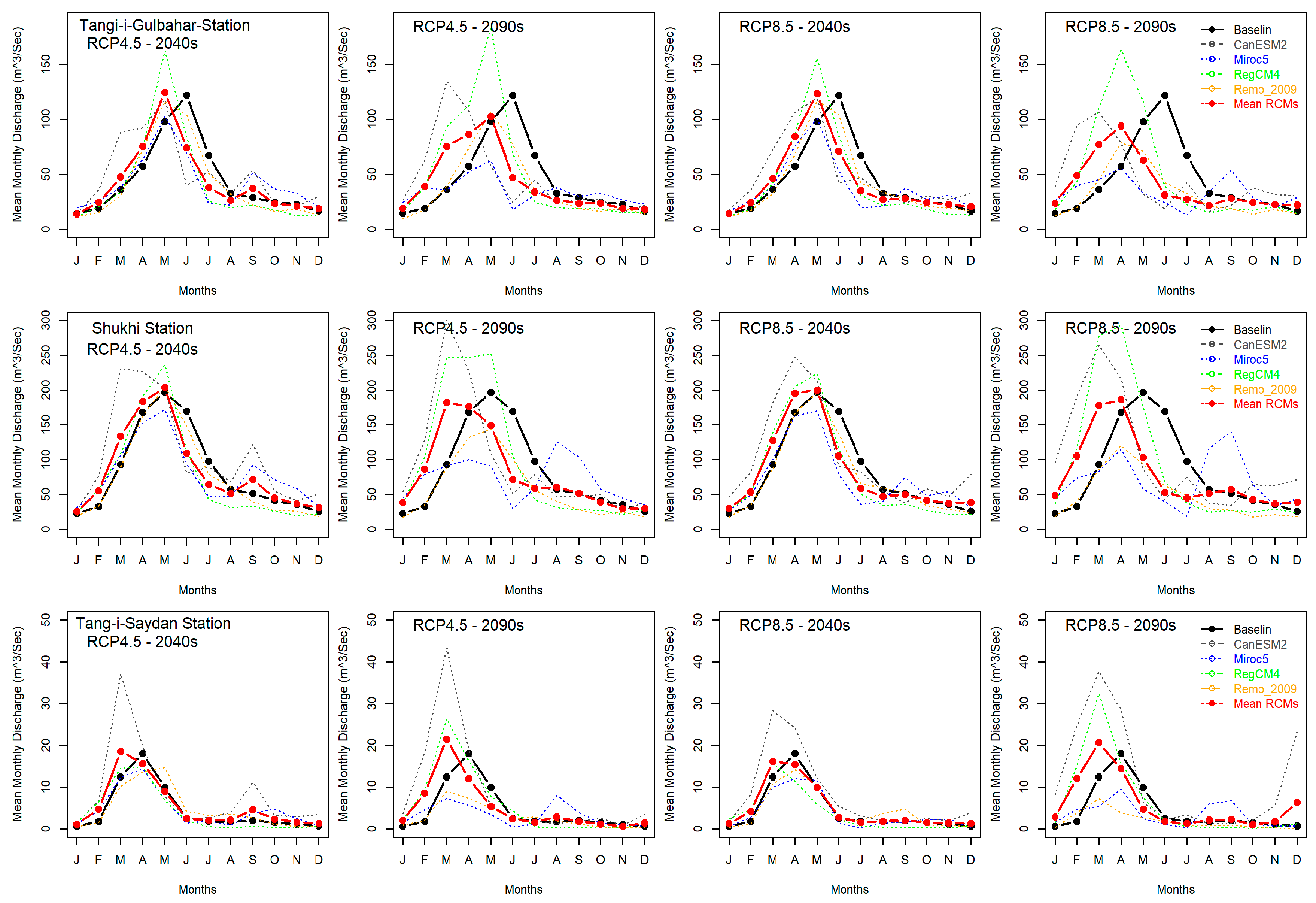
Figure 7 illustrates the response of climate change to the monthly surface runoff for the 2040s and 2090s under RCP4.5 and RCP8.5. The baseline (1968–2005) runoff is shown by the black line, and the model’s mean is shown by the red lines. Figure 7 indicates how the temperature’s increase impacted the runoff in the UKRB, subsequently causing a decrease in summer runoff and an increase in the winter and spring runoff. The future monthly maximum runoff also showed a shift to earlier months due to climate change in the UKRB. The monthly runoff shows a shift in March and April instead of May and June in Tang-I-Gulbahar and Shukhi stations, while in the Tang-i-Saidan station, the peak shifts from April to March can be seen in both periods of the 2040s and 2090s. In the 2090s, the water availability is projected to reduce compared to the 2040s under both scenarios of RCP4.5 and RCP8.5. The results from each RCM show a different pattern of monthly runoff. The CanESM-2 and the RegCM4-4 models are wetter climate models, which show higher discharge peaks compared to the baseline and the other models. In contrast, Miroc-5 and Remo-2009 showed a lower monthly discharge peak compared to the historical period and the other two RCMs. Based on the runoff results, the future seasonal water availability could be expected to vary in the UKRB. The results indicate that the changes in hydrological parameters tend to be more extreme under higher emission scenarios (RCP8.5) and in the end-century (2090s). In this scenario, the runoff values decreased further in the summer months compared to RCP4.5. The monthly future discharge is projected to increase in the first four months of the year (January to April) and decrease in the summer months (May to August). Specifically, the period of the 2090s is projected to be much drier under the RCP8.5 scenario compared to the RCP4.5 scenario, meaning a greater reduction in runoff in that period.

3.3.2. Seasonal Variations in Streamflow

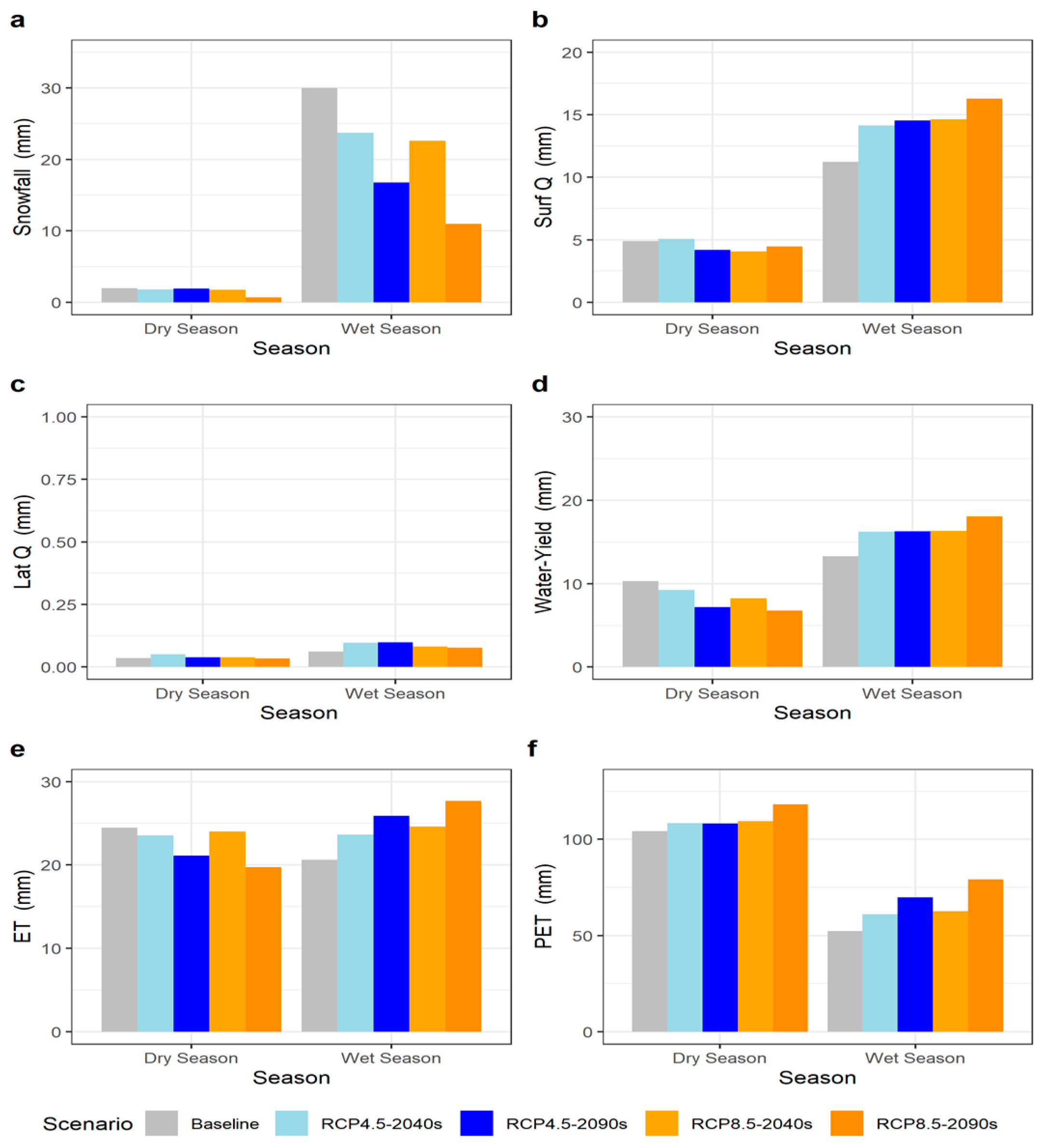
The future change in seasonal surface runoff and other hydrological parameters in the UKRB is presented in Figure 8. The seasonal runoff shows larger variations during the rainy season (December to May) compared to the dry season (June to November). Additionally, compared to the baseline, the amount of water flowing in the rivers during the winter and early spring (wet) seasons is increasing due to heavy precipitation and snowmelt; however, runoff decreases in the summer and autumn (dry) seasons. These streamflow increments were more accentuated in the rainy season and in the long term, with an increase of approximately 45% of streamflow under RCP8.5 for the period of the 2090s. The future seasonal lateral soil flow is expected to increase in both dry and wet seasons in the UKRB. In the wet season, the streamflow is also mainly determined by the increase in the baseflow contribution. The results show a seasonal snowfall reduction in both future periods of the 2040s and 2090s during the wet season. The seasonal actual evapotranspiration (ET) is expected to increase in winter and spring while showing a slight decrease during the summer and autumn seasons. The PET showed a seasonal increase in both the wet and dry seasons in the UKRB.

3.3.3. Annual Variations in Streamflow

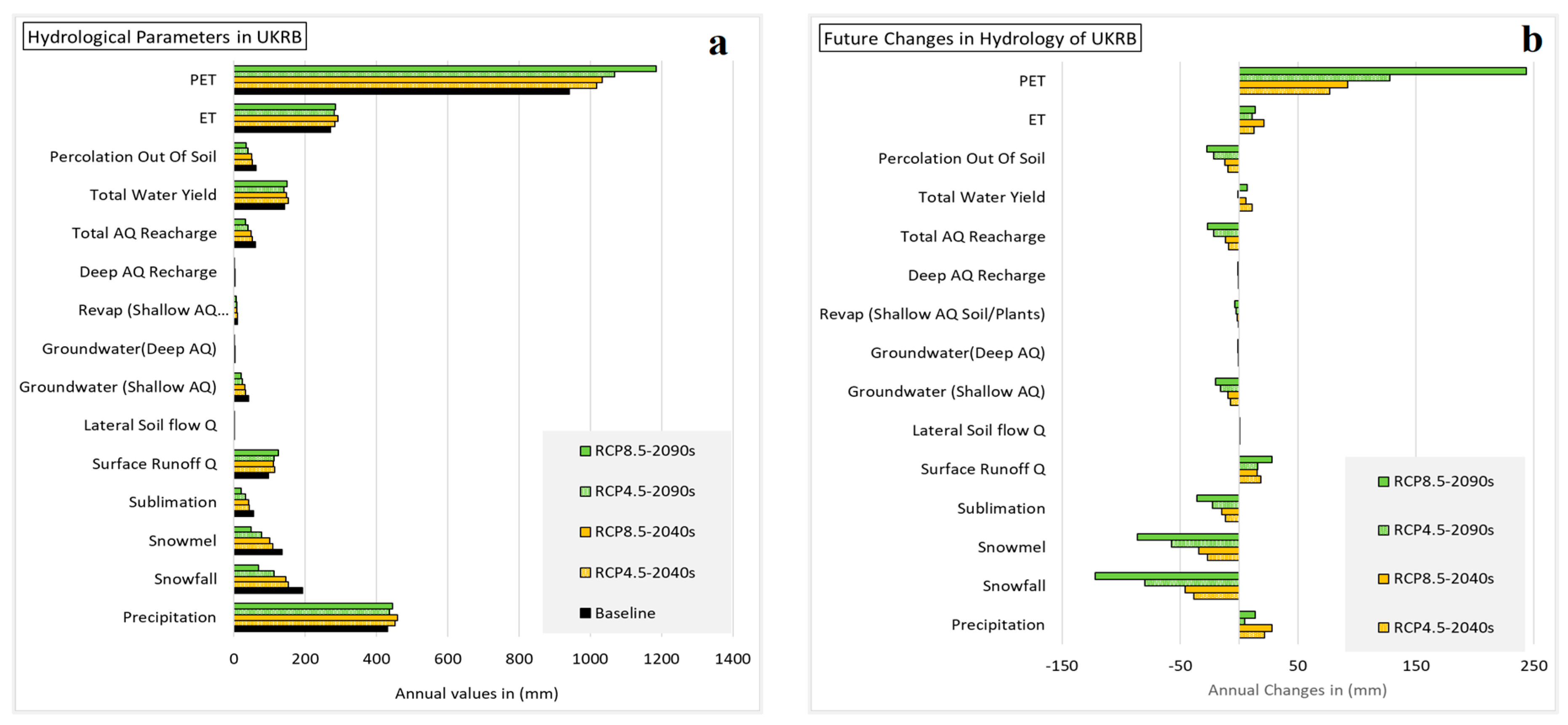
The future-projected annual changes in streamflow, percolation, ET, PET, snowfall, and snowmelt for the 2040s and 2090s under two RCP scenarios are depicted in Figure 9. The results indicate that there will be an increase in the annual streamflow and the total annual water yield in the 2040s and 2090s compared to the baseline due to an increase in total precipitation in the UKRB. The annual surface runoff throughout the UKRB is projected to increase by 18 mm in the 2040s and 15 mm in the 2090s compared to the baseline based on RCP4.5. Likewise, the annual surface runoff is projected to increase by 15 mm in the 2040s and 28 mm in the 2090s compared to the baseline under RCP8.5. In contrast, the annual snowfall, snowmelt, sublimation, percolation, and groundwater recharge showed a decrease compared to the baseline in the UKRB. The annual snowfall decreases included −38.5 mm and −80 mm for the 2040s and 2090s, respectively, under RCP4.5. In addition, snowfall is expected to decrease by −48 mm and −122 mm for the 2040s and 2090s, respectively, under RCP8.5.

The annual snowmelt indicated decreases of −26 mm and −57 mm for the 2040s and 2090s based on RCP4.5. Under RCP8.5, the annual snowmelt indicated a decrease of −34 mm and −86 mm for the 2040s and 2090s. The decrease in snowfall and snowmelt in the future could likely be due to the impact of climate change, specifically the increase in higher temperatures and changing patterns of precipitation from snowfall to rainfall in the UKRB. The snow and glaciers will melt faster and in the earlier months of the year. Also, both the snowfall and snowmelt show a maximum decrease in the 2090s under both RCPs 4.5 and 8.5. The results also show that percolation and the groundwater contribution to streamflow will decrease in the future. Under RCP4.5, the decrease in groundwater contribution is −7.5 mm and −15.8 mm for the 2040s and 2090s, respectively. Meanwhile, under RCP8.5, the decrease will be larger, with −9 mm and −20 mm for the same periods, respectively. These changes in groundwater and soil percolation have significant implications for the water resources in the UKRB, as they can affect the overall water availability and contribute to the changes in surface runoff.

The results also show that an increase in temperature is impacting the actual ET and PET. The annual ET and PET showed an increase in both RCP4.5 and RCP8.5 compared to the baseline in the UKRB. The ET increased under RCP4.5 by 13 mm in the 2040s and by 11 mm in the 2090s, while under RCP8.5, the ET significantly increased by 21 mm and 14 mm for the 2040s and 2090s, respectively. The increase in annual ET is more prominent in the 2090s under RCP8.5 (Figure 9). The annual lateral soil flow contribution is very low in the UKRB and, therefore, for the future, climate change analysis did not show any significant changes under both RCPs. Overall, the annual runoff is projected to increase; consequently, there will be more surface runoff in the basin annually, but there is also likely to be a problem with uneven seasonal and spatial distribution of water resources.

4. Discussion

The hydrological modeling performance refers to how accurately a model predicts the behavior of the system being studied compared to actual observations. The SWAT hydrological model is conducted by comparing the simulated results to the real-world discharge observations in the UKRB. The model was built, calibrated, and validated at monthly time intervals to provide a comprehensive analysis of the model’s accuracy. This type of evaluation is essential in ensuring that models are reliable tools for predicting the behavior of natural systems and can be used to make informed decisions. The statistical Nash–Sutcliffe (NS) efficiency performance of runoff was generally satisfactory, with good agreement between the simulated and observed discharge over the UKRB during calibration and validation according to Ref. [39], which stated that simulations in runoff are satisfactory when NSE is greater than 0.5, R² is great than 0.6 and PBIAS is in range of ±25%. Thus, all values of NSE, R₂, and PBIAS were compared with those recommended by [39]. However, we noticed that there was uncertainty in the model’s ability to simulate flow peaks, with underestimations occurring in some years at the calibrated stations (Figure 5). On the other hand, the simulated baseflow had a reasonable fit compared to observations in all calibrated stations except for the Pul-i-Ashawa station on the Ghorband River, where there was a higher baseflow in August and September compared to the observations. According to previous studies [39], underestimation in hydrological modeling occurs due to observation errors, biases in precipitation, and hydrological parameter uncertainties.

The monthly results showed that the model’s performance was good to very good in most of the stations, with monthly NS values ranging from 66% to 91%. However, the Sang-i-Nawishta station had a lower NS value of 54%, indicating that the model’s performance was only satisfactory in that station. The possible reasons behind the lower values of NS in the Sang-i-Nawishta station between observed and simulated runoff could be due to errors in the input precipitation used in the model. Studies show that the performance of the SWAT model at multi-outlets is poorer than that of a single outlet [41]. Overall, the SWAT model accurately observed river discharge during calibration and validation, although most peak flow months were underestimated, and the low flow months were overpredicted in the stations. This information provides an indication of the variability of the water flow in the KRB and can be used to validate the results of the hydrological model used in this study. The statistical results of SWAT indicated that the model is adequate for runoff estimation and simulating hydrology in the UKRB. The results conclude that SWAT has demonstrated its quality and potential as a numerical tool for water resource management in this study.

By inserting an input of 406 mm of average precipitation, the model simulation showed the output as 148.5 mm of the total water yield, accounting for 37% of the basin water balance. While, due to a larger PET of 1790 mm, the average ET was estimated to 246.6 mm (63%) and was greater than the total water yield (37%). The ET contribution was 63% of the total hydrological parameters that went back to the atmosphere rather than contributing to the water yield. The surface runoff accounts for 25%, and the total groundwater recharge accounts for 12% of the annual water yield in the study area. The study showed that between 2010 and 2019, ET was the major water loss component in the study area. In this study, the ET and groundwater were not validated during the hydrological model processing due to a lack of access to observed data. Thus, it seems reasonable to assume that these two critical components were well simulated but clearly consist of some minor uncertainty. Despite this, “very favorable” runoff results were achieved at multiple locations by the SWAT model.

The study compared the baseline period (1986–2005) with that of the future periods of the 2040s and 2090s under RCP4.5 and RCP8.5 scenarios. The results of our study reveal that an earlier shift in the future monthly runoff peaks is expected in both periods of the 2040s and 2090s. The runoff shifts in the hydrograph have similar patterns in both RCP scenarios. These shifts in the timing of runoff are due to the impact of climate change and can have significant effects on the availability of water resources for various sectors, such as agriculture, industry, and domestic consumption, which may further exacerbate water stresses in the study area. For instance, the shifts show that the snowmelt occurs earlier in the year, resulting in a rapid increase and a larger runoff for a shorter period, which may lead to more floods in the spring and droughts in the summer months. The Kabul River is a very small tributary of the very large Indus River, i.e., it is included in the basin of this river. It is quite clear that the water regime of the Indus River will have a decisive influence on the tributaries, including the Kabul River, in the future. Sohaib et al. [42] found future seasonal shifts in the streamflow and the rainfall shifts at the Nowshera and Chitral watershed of KRB, and Ref. [18] found that the peak hydrograph split into two peaks; one formed in Mar-Apr indicated earlier snowmelt, and the second one in August, which was due to Monsoon rains increased in the Alingar watershed of the KRB. Our study suggests that the total runoff in the UKRB is expected to increase under RCP4.5 and RCP8.5, except for the 2090s in the RCP8.5 scenario. According to the results, there will be an increase in annual streamflow in the 2040s and 2090s compared to the baseline in UKRB. Yao Chen et al. [43] studied the impact of climate change on hydrological regimes in the Yarlung Tsangp basin using SWAT and predicted the increasing trends of surface runoff and total surface runoff. The increment of annual surface runoff in the UKRB is due to an increase in the annual precipitation [43], and there are other factors that might offset this increase, for instance, a decrease in percolation and groundwater. Other factors, such as changes in temperature, could also potentially impact the hydrological cycle and contribute to changes in streamflow patterns [42]. Additionally, there will be a decrease in annual percolation and groundwater recharge, which could further reduce the water availability in the summer season.

The results show that both RCP4.5 and RCP8.5 scenarios project a decrease in annual snowfall, snow melting, and sublimation, with a larger decrease occurring in the 2090s. A decrease in snowfall and snow cover will particularly affect the recharges in alluvial fan aquifers from snowmelt in the KRB [44,45]. This decrease in snowmelt also leads to changes in the timing and volumes of river flow, which can impact the water availability for agriculture, urban consumption, and hydropower generation [9]. Therefore, while there is an increase in annual surface runoff, it might not necessarily translate to an overall increase in water availability as we see the 2090s under RCP8.5, which on the contrary, shows a very small decrease in the total water yield.

There has been a significant increase in the future ET and PET in the UKRB under both RCP4.5 and RCP8.5 scenarios. The increase in the ET is more prominent in the 2090s under RCP8.5, which implies that the projected future climate change will have more a significant impact on the ET. Studies in Pakistan, Nigeria, and Asian drylands [46,47,48] indicate that increases in evapotranspiration will accelerate the drought in these regions, particularly in the dry land of Asia. The evaporation variation was influenced by temperature and precipitation in UKRB. As temperature rose in the future scenarios, an increase in the ET was revealed. Increasing the rate of ET means that more water is lost from the land’s surface, resulting in a decrease in the amount of water available for surface runoff, groundwater recharge, and other hydrological processes, especially in the summer season. This is an important finding as ET plays a crucial role in the water balance of UKRB. This information is important in understanding the impacts of climate change on the hydrological cycle in the KRB and can aid in developing effective water management strategies. Our research findings are aligned with previous studies [49,50] conducted in this region.

The main result is that the annual discharge is projected to increase in the future, meaning there will be more surface runoff in the basin; however, the runoff increase may not be distributed evenly across seasons and spatially in the study area. This suggests that, while there may be an overall increase in the total water yield, except in the 2090s under RCP4.5, the groundwater recharge may decrease in the future, and there could still be challenges in managing and distributing water effectively. Additionally, compared to the baseline period, there will be an increase in the seasonal streamflow during the rainy season and decreases in the dry season. The studies [42,51,52] also suggest that summer flows will continue to drop in the future, whereas spring and winter flows will increase in the Indus River Basin. The seasonal variation in streamflow can lead to more frequent floods during the wet season and droughts during the dry season due to less runoff and a higher ET in the UKRB. In addition, there will be a larger gap between water availability and demand, particularly during the dry season (summer). This research indicates that water resources may not be sufficient to meet the demand during the summer season, which could lead to water scarcity issues. This is because water resources are not being adequately replenished during the dry season, leading to a water deficit.

5. Conclusions

This research investigated the impacts of climate change on water resources in the UKRB. The capability of the SWAT model was analyzed statistically and graphically. The performance of NSE, as an objective function during calibration, was good and acceptable in multiple stations, with NS values ranging from 66% to 91%. SWAT showed good agreement between the simulated and observed runoff in a scarce data region of the UKRB.

The modeling of future hydrological projections revealed the annual surface runoff and total runoff attributed to an increase in the 2040s and 2090s compared to the baseline period under both RCPs 4.5 and 8.5. The future annual temperature and precipitation also showed an increase in both periods and both RCPs. The increase in annual runoff is due to an increase in annual precipitation. The surface runoff is projected to increase by 16% (2040s) and 14% (2090s) compared to the baseline based on RCP4.5. Likewise, the surface runoff is projected to increase by 14% (2040s) and 22% (2090s) under RCP8.5. The total annual runoff (total water availability) showed an increase of 7% in the 2040s but a decrease of −4% for the 2090s under RCP4.5 and showed an increase of 4% and 5% in the 2040s and 2090s under RCP8.5. The future hydrographs indicated an earlier shift in monthly runoff peaks due to a temperature increase and changes in the precipitation pattern and amount. However, the study predicted decreases in annual snowfall, snowmelt, sublimation, percolation, and groundwater recharge. The decrease in groundwater’s contribution to streamflow was projected to −22% and −63% under RCP4.5 and −29% and 93% under RCP8.5 for the 2040s and 2090s, respectively. Snowfall is projected to decrease by −25% and −71% under RCP4.5 and 31% and 174% under RCP8.5 for the periods of the 2040s and 2090s, respectively. A decrease in snowfall will result in snowmelt in the UKRB. The decrease in snowmelt and melting of glaciers could also lead to changes in the timing and volumes of runoff, which will impact the water availability for agriculture, urban water consumption, and hydropower generation seasonally. The shifts in the timing of runoff will exacerbate water scarcity and water stress, especially as decreases shown in the summer runoff will increase floods due to the increased runoff in winter and spring seasons and the impact of climate change. Also, the seasonal runoff variation will increase the gaps between demand and water availability in the summer. Rising temperatures contribute to higher evaporation rates. The future evapotranspiration is anticipated to increase by 4%, 4% under RCP4.5 and 7%, and 5% under RCP8.5 for the 2040s and 2090s, respectively, in the UKRB. Increases in future temperature may also increase the salt concentration in remaining water bodies; however, we did not consider this in this study.

As a conclusion drawn from the findings of this study, climate change is expected to have significant impacts on water availability in the UKRB. The continued increase in temperature in the future will disrupt precipitation patterns from snowfall to rainfall, leading to accelerations in erratic precipitation and the melting of permanent snow and glaciers in the study area. This trend has implications for sustainable water resource management and hydrological disaster warnings in the study area and in the regions farther downstream. Moreover, the projected decrease in water availability, especially in summer, could lead to negative consequences on agriculture, livestock, and food security in the future if this is not managed. This imbalance in the seasonal availability of water resources can have significant implications for the management of water resources, including the need for appropriate infrastructures (e.g., check dams, ponds, and reservoirs), careful management and planning strategies, and effective water conservation practices to ensure sustainable water use, and to address the climate change risks. These findings highlight the need for and importance of implementing effective climate adaptation and mitigation strategies to help mitigate the impact of climate change on water resources in the study area. However, uncertainty remains regarding the groundwater and ET validation due to a lack of observed data. Also, future landcover change was not considered in this study for climate change modeling. It is hoped that subsequent studies will consider the groundwater and ET validation in modeling and changes in future landcover as well, if possible. Overall, these findings can aid policymakers and researchers who are working on climate change implication studies and water resources in the KRB and Afghanistan. Additionally, this study contributes to the growing body of knowledge on climate change’s impacts on water resources and emphasizes the need for continued research in this field.

References

1. IPCC. Summary for Policymakers. In Climate Change 2023: Synthesis Report. Contribution of Working Groups I, II and III to the Sixth Assessment Report of the Intergovernmental Panel on Climate Change; IPCC: Geneva, Switzerland, 2023. [Google Scholar]
2. IPCC. Summary for Policymakers. In Climate Change 2021: The Physical Science Basis. Contribution of Woring Group I to the Sixth Assessment Report of the Intergovernmental Panel on Climate Change; Masson-Delmotte, V., Zhai, P., Pirani, A., Connor, S.L., Eds.; Cambridge University Press: Cambridge, UK, 2021; Volume 9781107025, pp. 3–32. ISBN 9781139177245. [Google Scholar]
3. Sediqi, M.N.; Komori, D. Assessing Water Resource Sustainability in the Kabul River Basin: A Standardized Runoff Index and Reliability, Resilience, and Vulnerability Framework Approach. Sustainability 2023, 16, 246. [Google Scholar] [CrossRef]
4. Shiru, M.S.; Shahid, S.; Shiru, S.; Chung, E.S.; Alias, N.; Ahmed, K.; Dioha, E.C.; Sa’adi, Z.; Salman, S.; Noor, M.; et al. Challenges in water resources of lagos mega city of nigeria in the context of climate change. J. Water Clim. Chang. 2020, 11, 1067–1083. [Google Scholar] [CrossRef]
5. Arian, H.; Kayastha, R.B.; Bhattarai, B.C.; Shresta, A.; Rasouli, H.; Armstrong, R. Application of the Snowmelt Runoff Model in the Salang River Basin, Afghanistan Using MODIS Satellite Data. J. Hydrol. Meteorol. 2016, 9, 109–118. [Google Scholar] [CrossRef]
6. Bokhari, S.A.A.; Ahmad, B.; Ali, J.; Ahmad, S.; Mushtaq, H.; Rasul, G. Future Climate Change Projections of the Kabul River Basin Using a Multi-model Ensemble of High-Resolution Statistically Downscaled Data. Earth Syst. Environ. 2018, 2, 477–497. [Google Scholar] [CrossRef]
7. Iqbal, M.S.; Dahri, Z.H.; Querner, E.P.; Khan, A.; Hofstra, N. Impact of climate change on flood frequency and intensity in the kabul river basin. Geosciences 2018, 8, 114. [Google Scholar] [CrossRef]
8. Ahmad, I.; Tang, D.; Wang, T.; Wang, M.; Wagan, B. Precipitation trends over time using Mann-Kendall and spearman’s Rho tests in swat river basin, Pakistan. Adv. Meteorol. 2015, 2015, 431860. [Google Scholar] [CrossRef]
9. Sediqi, M.N.; Shiru, M.S.; Nashwan, M.S.; Ali, R.; Abubaker, S.; Wang, X.; Ahmed, K.; Shahid, S.; Asaduzzaman, M.; Manawi, S.M.A. Spatio-temporal pattern in the changes in availability and sustainability ofwater resources in Afghanistan. Sustainability 2019, 11, 5836. [Google Scholar] [CrossRef]
10. Goes, B.J.M.; Howarth, S.E.; Wardlaw, R.B.; Hancock, I.R.; Parajuli, U.N. Integrated water resources management in an insecure river basin: A case study of Helmand River Basin, Afghanistan. Int. J. Water Resour. Dev. 2016, 32, 3–25. [Google Scholar] [CrossRef]
11. Mew, J. Project for Capacity Enhancement on Hydro-Meteorological Information Management in the Ministry of Energy and Water in the Islamic Republic of Afghanistan; Japan International Cooperation Agency: Tokyo, Japan, 2019. [Google Scholar]
12. Akhtar, F.; Awan, U.K.; Borgemeister, C.; Tischbein, B. Coupling remote sensing and hydrological model for evaluating the impacts of climate change on streamflow in data-scarce environment. Sustainability 2021, 13, 14025. [Google Scholar] [CrossRef]
13. Akhtar, F.; Awan, U.K.; Tischbein, B.; Liaqat, U.W. Assessment of irrigation performance in large river basins under data scarce environment-A case of Kabul River basin, Afghanistan. Remote Sens. 2018, 10, 972. [Google Scholar] [CrossRef]
14. Ahmadzai, S.; McKinna, A. Afghanistan electrical energy and trans-boundary water systems analyses: Challenges and opportunities. Energy Rep. 2018, 4, 435–469. [Google Scholar] [CrossRef]
15. Qureshi, A. Water Resources Management in Afghanistan: The Issues and Options; International Water Management Institute: Colombo, Sri Lanka, 2002. [Google Scholar]
16. Hashmi, M.Z.U.R.; Masood, A.; Mushtaq, H.; Bukhari, S.A.A.; Ahmad, B.; Tahir, A.A. Exploring climate change impacts during first half of the 21st century on flow regime of the transboundary kabul river in the hindukush region. J. Water Clim. Chang. 2020, 11, 1521–1538. [Google Scholar] [CrossRef]
17. Sidiqi, M.; Kasiviswanathan, K.S.; Scheytt, T.; Devaraj, S. Assessment of Meteorological Drought under the Climate Change in the Kabul River Basin, Afghanistan. Atmosphere 2023, 14, 570. [Google Scholar] [CrossRef]
18. Akhtar, F.; Borgemeister, C.; Tischbein, B.; Awan, U.K. Metrics Assessment and Streamflow Modeling under Changing Climate in a Data-Scarce Heterogeneous Region: A Case Study of the Kabul River Basin. Water 2022, 14, 1697. [Google Scholar] [CrossRef]
19. Sidiqi, M.; Shrestha, S.; Ninsawat, S. Projection of climate change scenarios in the Kabul River Basin, Afghanistan. Curr. Sci. 2018, 114, 1304–1310. [Google Scholar] [CrossRef]
20. FAO-MAIL. Food and Agriculture Organization of the United Nations, Ministry of Agriculture, Irrigation and Livestock Landcover Atlas of the Islamic Rebulic of Afghanistan; FAO: Rome, Italy, 2010. [Google Scholar]
21. Aich, V.; Akhundzadah, N.A.; Knuerr, A.; Khoshbeen, A.J.; Hattermann, F.; Paeth, H.; Scanlon, A.; Paton, E.N. Climate change in Afghanistan deduced from reanalysis and coordinated regional climate downscaling experiment (CORDEX)-South Asia simulations. Climate 2017, 5, 38. [Google Scholar] [CrossRef]
22. Ghulami, M.; Babel, M.S.; Shrestha, M.S. Evaluation of gridded precipitation datasets for the Kabul Basin, Afghanistan. Int. J. Remote Sens. 2017, 38, 3317–3332. [Google Scholar] [CrossRef]
23. Teutschbein, C.; Seibert, J. Bias correction of regional climate model simulations for hydrological climate-change impact studies: Review and evaluation of different methods. J. Hydrol. 2012, 456–457, 12–29. [Google Scholar] [CrossRef]
24. Rathjens, H.; Bieger, K.; Srinivasan, R.; Chaubey, I.; Arnold, J.G. CMhyd User Manual Documentation for Preparing Simulated Climate Change Data for Hydrologic Impact Studies; SWAT: Garland, TX, USA, 2016. [Google Scholar]
25. Arnold, J.G.; Srinivasan, R.; Muttiah, R.S.; Williams, J.R. Large area hydrologic modeling and assessment part I: Model development. J. Am. Water Resour. Assoc. 1998, 34, 73–89. [Google Scholar] [CrossRef]
26. Srinivasan, R.; Ramanarayanan, T.S.; Arnold, J.G.; Bednarz, S.T. Large area hydrologic modeling and assessment part II: Model application. J. Am. Water Resour. Assoc. 1998, 34, 91–101. [Google Scholar] [CrossRef]
27. Winchell, M.; Srinivasan, R.; Di Luzio, M.; Arnold, J.G. ArcSWAT User’s Guide; Blackland Research and Extension Center: Temple, TX, USA, 2013; p. 464. [Google Scholar]
28. Ayoubi, T.; Dongshik, K. Panjshir watershed hydrologic model using integrated gis and panjshir watershed hydrologic model using. J. Earth Environ. Sci. 2016, 6, 145–161. [Google Scholar]
29. Mengistu, A.G.; van Rensburg, L.D.; Woyessa, Y.E. Techniques for calibration and validation of SWAT model in data scarce arid and semi-arid catchments in South Africa. J. Hydrol. Reg. Stud. 2019, 25, 100621. [Google Scholar] [CrossRef]
30. Kouchi, D.H.; Esmaili, K.; Faridhosseini, A.; Sanaeinejad, S.H.; Khalili, D.; Abbaspour, K.C. Sensitivity of calibrated parameters and water resource estimates on different objective functions and optimization algorithms. Water 2017, 9, 384. [Google Scholar] [CrossRef]
31. Zhou, P.; Huang, J.; Pontius, R.; Hong, H. Soil and Water Assessment Tool Theoretical Documentation Version 2009. Sci. Total Environ. 2016, 543, 591–600. [Google Scholar] [CrossRef]
32. Wu, J.; Zheng, H.; Xi, Y. SWAT-based runoff simulation and runoff responses to climate change in the headwaters of the Yellow River, China. Atmosphere 2019, 10, 509. [Google Scholar] [CrossRef]
33. Abbaspour, K.C.; Rouholahnejad, E.; Vaghefi, S.; Srinivasan, R.; Yang, H.; Kløve, B. A continental-scale hydrology and water quality model for Europe: Calibration and uncertainty of a high-resolution large-scale SWAT model. J. Hydrol. 2015, 524, 733–752. [Google Scholar] [CrossRef]
34. Abbaspour, K.C.; Johnson, C.A.; van Genuchten, M.T. Estimating Uncertain Flow and Transport Parameters Using a Sequential Uncertainty Fitting Procedure. Vadose Zone J. 2004, 3, 1340–1352. [Google Scholar] [CrossRef]
35. Abbaspour, K.C. SWAT-CUP SWATCalibration and Uncertainty Programs; Eawag: Dübendorf, Switzerland, 2015; pp. 2–100. [Google Scholar]
36. Nash, J.E.; Sutcliffe, J.V. River flow forecasting through conceptual models part I—A discussion of principles. J. Hydrol. 1970, 10, 282–290. [Google Scholar] [CrossRef]
37. Yapo, P.O.; Gupta, H.V.; Sorooshian, S. Automatic calibration of conceptual rainfall-runoff models: Sensitivity to calibration data. J. Hydrol. 1996, 181, 23–48. [Google Scholar] [CrossRef]
38. Gupta, H.V.; Kling, H.; Yilmaz, K.K.; Martinez, G.F. Decomposition of the mean squared error and NSE performance criteria: Implications for improving hydrological modelling. J. Hydrol. 2009, 377, 80–91. [Google Scholar] [CrossRef]
39. Moriasi, D.N.; Arnold, J.G.; Van Liew, M.W.; Bingner, R.L.; Harmel, R.D.; Veith, T.L. Model Evaluation Guidelines for Systematic Quantification of Accuracy in Watershed Simulations. Trans. ASABE 2007, 50, 885–900. [Google Scholar] [CrossRef]
40. Arnold, J.G.; Kiniry, J.R.; Srinivasan, R.; Williams, J.R.; Haney, E.B.; Neitsch, S.L. Input/Output Documentation Soil & Water Assessment Tool; Texas Water Resources Institute: Thrall, TX, USA, 2012; pp. 1–650. [Google Scholar]
41. Li, K.; Wang, Y.; Li, X.; Yuan, Z.; Xu, J. Simulation effect evaluation of single-outlet and multi-outlet calibration of Soil and Water Assessment Tool model driven by Climate Forecast System Reanalysis data and ground-based meteorological station data—A case study in a Yellow River source. Water Sci. Technol. Water Supply 2021, 21, 1061–1071. [Google Scholar] [CrossRef]
42. Baig, S.; ul Hasson, S. Flood Inundation and Streamflow Changes in the Kabul River Basin under Climate Change. Sustainability 2023, 16, 116. [Google Scholar] [CrossRef]
43. Chen, Y.; Wang, L.; Shi, X.; Zeng, C.; Wang, Y.; Wang, G.; Qiangba, C.; Yue, C.; Sun, Z.; Renzeng, O.; et al. Impact of Climate Change on the Hydrological Regimes of the Midstream Section of the Yarlung Tsangpo River Basin Based on SWAT Model. Water 2023, 15, 685. [Google Scholar] [CrossRef]
44. Macpherson, G.L.; Johnson, W.C.; Liu, H. Viability of karezes (ancient water supply systems in Afghanistan) in a changing world. Appl. Water Sci. 2017, 7, 1689–1710. [Google Scholar] [CrossRef]
45. Casale, F.; Bombelli, G.M.; Monti, R.; Bocchiola, D. Hydropower potential in the Kabul River under climate change scenarios in the XXI century. Theor. Appl. Climatol. 2020, 139, 1415–1434. [Google Scholar] [CrossRef]
46. Waseem, M.; Ajmal, M.; Ahmad, I.; Khan, N.M.; Azam, M.; Sarwar, M.K. Projected drought pattern under climate change scenario using multivariate analysis. Arab. J. Geosci. 2021, 14, 1–13. [Google Scholar] [CrossRef]
47. Shiru, M.S.; Shahid, S.; Dewan, A.; Chung, E.S.; Alias, N.; Ahmed, K.; Hassan, Q.K. Projection of meteorological droughts in Nigeria during growing seasons under climate change scenarios. Sci. Rep. 2020, 10, 10107. [Google Scholar] [CrossRef]
48. Bonacci, O.; Bonacci, D.; Roje-Bonacci, T.; Vrsalović, A. Proposal of a new method for drought analysis. J. Hydrol. Hydromech. 2023, 71, 100–110. [Google Scholar] [CrossRef]
49. Giang, P.Q.; Toshiki, K.; Sakata, M.; Kunikane, S.; Vinh, T.Q. Modelling climate change impacts on the seasonality of water resources in the upper Ca river watershed in Southeast Asia. Sci. World J. 2014, 2014, 279135. [Google Scholar] [CrossRef] [PubMed]
50. Lutz, A.F.; Immerzeel, W.W.; Shrestha, A.B.; Bierkens, M.F.P. Consistent increase in High Asia’s runoff due to increasing glacier melt and precipitation. Nat. Clim. Chang. 2014, 4, 587–592. [Google Scholar] [CrossRef]
51. Lutz, A.F.; Immerzeel, W.W.; Kraaijenbrink, P.D.A.; Shrestha, A.B.; Bierkens, M.F.P. Climate change impacts on the upper indus hydrology: Sources, shifts and extremes. PLoS ONE 2016, 11, e0165630. [Google Scholar] [CrossRef] [PubMed]
52. Wijngaard, R.R.; Lutz, A.F.; Nepal, S.; Khanal, S.; Pradhananga, S.; Shrestha, A.B.; Immerzeel, W.W. Immerzeel Future changes in hydro-climatic extremes in the Upper Indus, Ganges, and Brahmaputra River basins. PLoS ONE 2017, 12, e0190224. [Google Scholar] [CrossRef] [PubMed]
Figure 1. Location of study area (Upper Kabul River Basin) in Afghanistan.
Atmosphere 15 00361 g001
Figure 2. (a) The land use, (b) soil classifications, (c) hydro-meteorological station’s location, and (d) APHRODITE-selected station’s map in the UKRB.
Atmosphere 15 00361 g002
Figure 3. Flowchart for the processing of data, model setup, calibration, and validation in UKRB.
Atmosphere 15 00361 g003
Figure 4. The monthly maximum and minimum temperatures after bias correction were obtained from RCMs under two RCP4.5 and RCP8.5 scenarios. The baseline period is represented by the black line, while the mean from the RCMs is shown by the red line.
Atmosphere 15 00361 g004
Figure 5. The monthly simulated and observed streamflow correlations for (a) Tangi-Gulbahar, (b) Pul-i-Ashawa, (c) Shukhi, (d) Tang-i-Gharu, (e) Tang-i-Saidan, and (f) Sang-i-Nawishta stations during the calibration (2010–2016) and validation (2017–2018) period. The calibration and validation periods are separated by horizontal dashed lines within the graphs.
Atmosphere 15 00361 g005
Figure 6. The simulated water balance components for monthly (a) and annual (b) periods in the UKRB.
Atmosphere 15 00361 g006
Figure 7. Future response of water flow compared to the baseline plots under RCP4.5 and RCP8.5 for Tang-i-Gulbahar station, Shukhi station, and Tangi-Saidan station. The black line shows the discharge for the baseline (1986–2005), and the red line shows the discharge for mean RCMs in two future periods of the 2040s and 2090s.
Atmosphere 15 00361 g007
Figure 8. The seasonal changes in (a) snowfall, (b) surface runoff, (c) lateral flow, (d) total water yield, (e) ET, and (f) PET for dry and wet seasons in the UKRB. The results are shown for the baseline, 2040s, and 2090s periods under RCP4.5 and RCP8.5.
Atmosphere 15 00361 g008
Figure 9. (a) The annual hydrological components and (b) changes in annual hydrological components for the 2040s and 2090s compared to the baseline under RCP4.5 and RCP8.5.
Atmosphere 15 00361 g009