Effects of Dust Storm and Wildfire Events on Phytoplankton Growth and Carbon Sequestration in the Tasman Sea, Southeast Australia

Abstract

Dust storms and wildfires occur frequently in south-eastern Australia. Their effects on the ecology, environment and population exposure have been the focus of many studies recently. Dust storms do not emit ground-sequestered carbon, but wildfires emit significant quantities of carbon into the atmosphere. However, both natural events promote phytoplankton growth in water bodies because carbon, and other trace elements such as iron, deposit on the surface water of oceans. Carbon dioxide is reabsorbed by phytoplankton via photosynthesis. The carbon balance cycle due to dust storms and wildfires is not well known. Recent studies on the carbon emission of the 2019–2020 summer wildfires in eastern Australia indicated that this megafire event emitted approximately 715 million tonnes of CO₂ (195 Tg C) into the atmosphere from burned forest areas. This study focusses on the association of dust storms and wildfires in southeastern Australia with phytoplankton growth in the Tasman Sea due to the February 2019 dust storm event and the 2019–2020 Black Summer wildfires. Central Australia and western New South Wales were the sources of the dust storm emission (11 to 16 February 2019), and the Black Summer wildfires occurred along the coast of New South Wales and Victoria (from early November 2019 to early January 2020). The WRF-Chem model is used for dust storm simulation with the AFWA (Air Force Weather Agency of the US) dust emission version of the GOCART model, and the WRF-Chem model is used for wildfire simulation with FINN (Fire Emission Inventory from NCAR) emission data. The results show the similarities and differences in the deposition of particulate matter, phytoplankton growth and carbon reabsorption patterns in the Tasman Sea from these events. A higher rate of deposition of PM_2.5 on the ocean surface corresponds to a higher rate of phytoplankton growth. Using the WRF-Chem model, during the 5-day dust storm event in February 2019, approximately ~1230 tons of total dust was predicted to have been deposited in the Tasman Sea, while ~132,000 tons of PM₁₀ was deposited in the early stage of the wildfires from 1 to 8 November 2019.

1. Introduction

Emissions of dust from dust storms and smoke aerosols from biomass burnings contain organic compounds and elemental metals including iron (Fe). The deposition of dust and aerosol particles of various sizes, such as PM_2.5 (particulate matter ≤ 2.5 μm in diameter) and PM₁₀ (particulate matter ≤ 10 μm in diameter), on the ocean increases the concentration of soluble Fe in marine water as these particles are transported from land sources over the ocean. One-third of the world’s oceans, particularly the high-nutrient low-chlorophyll (HNLC) Southern Ocean, is mostly iron-limited in stimulating phytoplankton growth [1]. The increase in the concentration of Fe stimulates the growth of phytoplankton (especially diatoms), which absorb CO₂ during photosynthesis [2]. This results in an increase in the CO₂ transferred from the atmosphere into the ocean. Phytoplankton as microalgae plants contain the chlorophyll pigment. Like other land-based plants, phytoplankton grows by absorbing carbon dioxide in sea water and producing glucose and oxygen through photosynthesis. Therefore, the chlorophyll concentration can be used as an index of the phytoplankton biomass. It is estimated that marine phytoplankton captures an amount of carbon that is almost equal to that captured by land vegetation via photosynthesis [3].

The global climate change models take Into account the ocean’s important role of carbon sequestration in the Global Carbon Cycle. The absorption of CO₂ via the phytoplankton life cycle is part of this process. Of the two main types of phytoplankton, dinoflagellates and diatoms, diatoms can grow quickly in an Fe-rich environment [4]. Recently, Gregg and Rousseaux, 2019 [5], have shown that satellite records indicated, from 1998 to 2015, the global net ocean primary production (PP), representing the uptake of inorganic carbon through photosynthesis, experienced a small but significant decline. This is mainly due to the changes in the compositions of types of phytoplankton. Using the sediment core record in the Southern Hemisphere, Calvo et al. 2004 [6] showed that increasing the supply of dust in the Tasman Sea during the last four glacial times, with different proportions of iron and silica, induced changes in the relative contribution of the types of phytoplankton to their total productivity. Besides its role in carbon sequestration, phytoplankton growth produces dimethylsulfide, which is emitted and, when entered into the atmosphere, can promote cloud formation and hence cool the atmosphere.

In early 2004, the European Iron Fertilization Experiment (EIFEX) stimulated a large-scale diatom bloom in the Southern Ocean near Antarctica, with peaks shown in the fourth week after fertilisation. This was followed by the mass mortality of several diatom species and resulted in rapidly sinking aggregates of entangled cells and chains. At least half the bloom biomass sank far below a depth of 1000 m with a substantial portion likely to have reached the sea floor [7]. This pioneering experiment showed the important role of the ocean and particularly of phytoplankton in the CO₂ absorption as part of the carbon cycle and the ideas of geo-engineering using Fe fertilisation for CO₂ sequestration [4,8]. The sequestration of CO₂ from the surface to deep water in the Southern Ocean via the biological pump gradually increases the dissolved inorganic carbon (DIC) concentration, such as the [CO₃]²⁻ in the oceanic carbon reservoirs.

In a study of the sediment core from the Subantarctic Atlantic, Martínez-García et al. (2014) [9] found that peak glacial times and millennial cold events are characterised by increases in the dust flux, consistent with subantarctic iron fertilisation. This resulted in the lowering of CO₂ at the transition from mid-climate states to full ice age conditions. Over time, circulation and ventilation via the upwelling of deep-water masses can alter between a carbon sink or source. The upwelling of Circumpolar Deep Waters (CDWs) in the Antarctic and Subantarctic Zones of the Southern Ocean can bring the carbon-rich waters in these reservoirs to the surface and release CO₂ into the atmosphere [10].

A recent modelling study by [11] on ocean dynamics showed that, depending on the depth at which carbon was stored, the median sequestration time driven by biological pump enhancement ranges from a few decades to ∼150 years with a global mean value of 109 years. The Atlantic and Southern Oceans have sequestration times shorter than the Pacific and Indian Oceans as deep upwelling occurs more frequently in the Southern Ocean. At a depth of 2100 m, more than 95% of the material remains sequestered after 50 years, and at a 3000 m depth, essentially 100% of the CO₂ is retained after 50 years.

The near-surface concentration of chlorophyll-a (milligrams of chlorophyll pigment/m³) in the ocean is detected via a colour change from blue to green and measured daily by sensors on polar-orbited MODIS Terra/Aqua satellites with a high resolution at 1 km × 1 km and a geostationary Himawari satellite over Australia to Japan at a time resolution of minutes. Phytoplankton grows when nutrients, including Fe, in the water are sufficient and temperature and light are favourable. If too many nutrients are present, this will result in high growth and a higher concentration of phytoplankton. Some species of phytoplankton can produce toxin build up, causing the algal bloom to deplete oxygen concentrations, which can be deadly to marine life and even people on land-based water bodies.

The composition of pollutants in the dust can also influence the solubility of Fe. Rodriguez et al. 2021 [12] studied the changing concentration of soluble Fe across the Atlantic Ocean from a dust storm outbreak in North Africa and found that dust mixing with acid pollutants increases the solubility of Fe. Dust storms from different sources therefore have different effects on the receiving water bodies, which themselves have different characteristics including nutrient levels. Lauderdale et al. 2020 [13] have recently shown that Fe fertilisation in the Southern Ocean, where rich nutrients such as nitrate and phosphate are readily available, overall cannot reduce atmospheric CO₂ and therefore cannot mitigate climate change as the world oceans are interconnected. For example, an increase in phytoplankton growth in the Southern Ocean due to iron fertilisation can reduce the availability of macronutrients in the North Atlantic and therefore reduce the phytoplankton growth there. Perron et al. 2020 [14] have shown that dust-sourced high Fe loadings and low-Fe-solubility (5%) aerosols dominate the atmospheric burden of the western coasts of Australia. However, there were much lower Fe concentrations but greater Fe solubilities (10.5% and 13%) in aerosols along the east coast, which was attributed to solubility-enhancing atmospheric reactions with anthropogenic pollutants. In northern Australia, high aerosol Fe solubilities (>20%) were associated with direct emissions or atmospheric reactions with bushfire emissions at tropical latitudes.

For some of the most significant dust storms on the east coast of Australia, such as the September 2009 “Red Dawn” dust storm event, Gabric et al. 2015 [15] found that surface chlorophyll concentrations in the southern Tasman Sea during the austral spring of 2009 were well above the climatological mean, with positive anomalies as high as 0.5 mg m⁻³. Earlier dust storms in late 2002 and early 2003 were also studied by Gabric et al. 2010 [16] using satellite data and the integrated wind erosion and dust transport model (CEMSYS) to simulate the daily deposition during November 2002 to February 2003. They found that during February 2003 there was strong evidence for a large-scale natural dust fertilization event in the Australian sector of the Southern Ocean.

The most recent major dust storm occurred in February 2019. In the austral summer of 2019, from 11 and 15 February 2019, under persistent westerly and south-westerly winds, a dust storm started in the deserts of central Australia and carried a large volume of dust in an extensive front of approximately 1500 km moving to the western region of the state of New South Wales (NSW) then to the coast, including the metropolitan area of Sydney, causing extremely high particle pollution. The dust continued to be transported across the Tasman Sea to New Zealand and to Antarctica [17]. This study will examine the effect of the February 2019 dust storm on the phytoplankton growth in the Tasman Sea.

Dust deposition is the largest source of Fe in the ocean basins by far, larger than the pyrogenic sources (fires and anthropogenic combustion). In a study on the trend of soluble Fe deposition from these sources based on satellite data from 1980 to 2005, Hamilton et al. 2020 [18] showed that dust iron decreases while fire iron slightly increases and anthropogenic iron has a significant increasing trend.

While dust iron dominates the absolute deposition magnitude, wildfire iron is an important contributor to temporal variability. The recent large wildfires on the east coast of Australia in the late spring and summer period of 2019/2020 (Black Summer wildfires) has been shown by Tang et al. 2021 [19] to contribute to significant growth of phytoplankton in the Pacific and South Australia parts of the Southern Ocean.

The Black Summer 2019/2020 wildfire event in southeast Australia was unprecedented in terms of scale or intensity, the duration of the fires and their spatial extent. With a prolonged drought in 2019, a low soil moisture and an increasing fuel load, the wildfires started in the northern coastal areas of NSW and the Blue Mountains areas of the state of NSW from late October and November to December 2019. Then, the wildfires occurred in the south coast of NSW, moving south to the coastal border areas between NSW and the state of Victoria and finally to East Gippsland area of Victoria in early January 2020 [20]. The 2019/2020 wildfires totally burned 5.68 million ha in NSW and 1.58 million hectares (ha) in Victoria [21] (Davey et al., 2020), and thirty-three people who lived in the vicinity of the fires lost their lives [22] (AIHW, 2020). People living in the wildland–urban interface (WUI) have a higher risk to their life and greater impact to their health and properties from wildfires. WUI areas are increasing in many parts of the world, including Australia and the US [23]. Fire policy targeting fire prevention, evacuation planning, fuel management and home hardening in the WUI areas has been implemented in the US to reduce the fire occurrence, risks to life loss and infrastructure damages [24].

The megafire of 2019/2020 emitted approximately 400 megatons (trillion or 10¹² g) of CO₂ into the atmosphere as estimated by the ECMWF (European Centre for Medium-Range Weather Forecasts) [https://atmosphere.copernicus.eu/wildfires-continue-rage-australia, accessed on 28 January 2024 ] [25]. Smoke aerosols rose to the upper troposphere more than 5 km above the ground and even to the stratosphere, travelling at a high speed to the South Pacific to South America to South Africa and back to the Australian continent. The effect of the megafire was compared to those of volcanic eruptions, which influenced the ENSO development cycles and hence had a far-reaching effect on the climate in many regions around the world [26]. Using coupled climate model ensembles based on the Community Climate System Model version 2 (CESM2), Fasullo et al. 2023 [26] have shown that the aerosol effect in the South Pacific from cloud formation and reflection cooled the atmosphere and the ocean surface temperature and prolonged the La Nina phase of the ENSO cycle.

To estimate the dispersion, transport and deposition of pollutants from the air to the surface level from dust or wildfire events, air quality models are often used. The two most common models are the WRF-Chem (Weather Research Forecast—Chemistry) and WRF-CMAQ (Weather Research Forecast—Community Multiscale Air Quality Modelling System) models. The WRF-CMAQ air quality model was used by many authors to study the deposition of pollutants. Qiao et al. 2015 [27] have used the WRF-CMAQ model to study the dry and wet deposition of sulfate, nitrate and ammonium ions in the Jiuzhaigou National Nature Reserve (China). Van der Velde et al. 2021 [28] have used the WRF-Chem v.4 model to estimate the emission and concentration of CO and CO₂ over eastern Australia during the 2019–2020 wildfires based on five different fire emission inventories where the emission estimate was constrained by CO satellite measurements. The WRF-Chem v.4 model was also used to study the effect of the 2019/2020 wildfires on the air quality and health in the east coast of Australia [16] and the transport of dust from the February 2019 dust storm to the Tasman Sea and Antarctica [17]. Kumar et al. 2023 [29] have recently used the WRF model to simulate the wind and surface meteorology to study the 2007 Witch Creek wildfire in California. They found that the planetary boundary layer (PBL) scheme Mellor-Yamada-Nakanishi-Niino (MYNN) yielded a better accurate prediction of surface meteorology than that of the PBL Yonsei University (YSU) scheme.

The WRF-Chem model has been used with different dust emission schemes to account for the dust emission and deposition in air quality dispersion models over a simulation domain [30,31]. The emission of dust created from wind erosion of the land surface is described as a function of the wind speed threshold, the soil characteristics, such as its type or texture and moisture content, and the dust source function (DSF), which describes the spatial erodibility of the land surface. This erodibility factor of the land depends on the land cover and, more specifically, the sediment supply. There are a number of methods to determine the erodibility at each location based on various hypotheses. The most common one is the topographic hypothesis, which calculates the erodibility (or sediment supply) based on the elevation at which topographic depressions are the largest sources of dust. This DSF based on the topographic hypothesis is called the Ginoux dust source function [32]. There are other hypotheses, such as the geomorphic one, which describes erodibility as a function of the upstream catchment area; the hydrologic hypothesis in which erodibility is described as a function of upstream flow; and, finally, the levelness hypothesis, which assumes that low-slope areas are the most conducive to dust formation [33]. The DSF used by the dust emission scheme options in the WRF-Chem air quality model is based on the topographic hypothesis.

Our study will focus on the effect of the early stage of the Black Summer wildfires in early November 2019 on the dispersion and deposition of smoke aerosols associating with the phytoplankton growth and subsequent carbon sequestration in the Tasman Sea. The objective of this study is to determine the association between dust and wildfire smoke particles’ deposition and phytoplankton growth in the Tasman Sea. For this purpose, the dust storms of February 2019 and the early stage of the Black Summer 2019–2020 wildfire events in early November 2019 and their effects on the atmospheric and marine environments are studied by using the WRF-Chem 4.2 air quality model. The model is used to simulate the dust fluxes generated from wind erosion and the dust transport and dispersion in the atmosphere, as well as the dust deposition on the land surface or ocean. Similarly, the wildfire event of summer 2019–2010 on the east coast of Australia was simulated using the WRF-Chem model and FINN (Fire Emission Inventory from NCAR) emission datasets [20].

The effects of these events on the biological processes in the Tasman Sea and beyond have not been examined before. Temporal and spatial quantities of PM_2.5 and PM₁₀ and the total dust from wildfires and dust emitted from these natural events and their deposition on the Tasman Sea off the southeast coast of Australia will be estimated from the simulation. The simulated results from both models will be compared with the observed patterns of phytoplankton growth as measured by polar-orbited MODIS Aqua/Terra and geostationary Himawari satellites and the phytoplankton data product from the Climate Change Initiative (CCI)—Ocean Colour of the European Space Agency (ESA). From these comparisons, the link and relationship between particle deposition and phytoplankton growth over time will be determined. And, hence, the WRF-Chem model can allow one to quantify the relationship between the emission and deposition of dust or smoke aerosols and the growth of phytoplankton in the ocean.

2. Materials and Methods

The data used for input into the WRF-Chem model consist of meteorological reanalysis data final analysis (FNL) from the National Center for Environmental Prediction (NCEP) of the US. Fire emission data are from the FINN (http://www.acom.ucar.edu/acresp/MODELING/finn_emis_txt/, accessed on 27 March 2021). Meteorological and air quality data are from the NSW Air Quality Monitoring Network, and satellite data (MODIS, CALIPSO) were used in our previous studies [17,20] to validate the WRF-Chem prediction.

Spatial data on chlorophyll-a were obtained from the NASA MODIS Aqua/Terra satellite chlorophyll-a product (https://worldview.earthdata.nasa.gov/, accessed on 2 January 2024) and from the Himawari geostationary satellite of the Japan Aerospace Exploration Agency (JAXA) (https://www.eorc.jaxa.jp/ptree/index.html, accessed on 2 January 2024). The Ocean Colour—Climate Change Initiative (OC-CCI) Project by the European Space Agency (ESA) in 2019 provided a merged multi-sensor record spanning 22 years, with time series of chlorophyll-a data from various satellite products of reflectance sensors. The OC-CCI data can be downloaded from https://rsg.pml.ac.uk/thredds/ncss/grid/CCI_ALL-v5.0-8DAY/dataset.html (accessed on 2 January 2024).

To determine the causal relationship between the dust storm and the phytoplankton growth in the Tasman Sea, the simulated dust deposition over the Tasman Sea between Australia and New Zealand for the period from 12 February 2019 to 15 February 2019 will be compared with observed chlorophyll-a data. The spatial and temporal high-resolution data product of the Climate Change Initiative (CCI)—Ocean Colour from the European Space Agency (ESA) combines various data sources, including those of NASA products, such as NASA OBPG SeaWiFS, NASA OBPG VIIRS L1 R2018.0 and NASA OBPG MODIS Aqua L1 R2018.0. These observed climate variables including chlorophyll-a are provided on an accessible and flexible open data portal platform for climate change research. This high-quality and high-resolution global dataset was subsetted for the Australian domain and was downloaded to be used as observed chlorophyll-a data in comparison with the predicted deposition of dust on the ocean surface.

In this study, we use the WRF-Chem V4.2 model to simulate the dust events of February 2019. The WRF-Chem dust emission scheme used is the AFWA (Air Force Weather Agency of the US) version of the GOCART (Goddard Chemistry Aerosol Radiation and Transport) model that we used in our previous study of dust transport from Australia to New Zealand and Antarctica [17]. This dust emission scheme is one of several dust emission options available in the WRF-Chem model.

In the AFWA-GOCART emission scheme (dust_opt = 3), the emission fluxes for the 5 particle size bins are stored in 4-dim DUST1, DUST2, DUST3, DUST4 and DUST5 variables with units in µg/kg of dry air. The dust emission generated over the domain is calculated as follows [34].

The accumulated dust emission (kilograms per cell) from each surface grid cell is given by the following:

$${EmisDUST1}_{i,j}={\sum }_{t=1}^n{DUST1}_{i,j}\times S_{i,j}\times \rho$$

(1)

where Emis DUST1_i,j is the dust flux at the surface for bin 1 at grid cell (i,j), t is the time step from 1 to n, S_i,j is the cell surface area (m²) and ρ is the air density.

Similarly, the gravitational settling (grav. settled DUST1, kg) and dry deposition (dry deposited DUST1, kg) are calculated for dust bin 1 using the following formulas:

$${Grav.Settled DUST1}_{i,j}={\sum }_{t=1}^n{GRASET\_1}_{i,j}\times S_{i,j}\times \rho$$

(2)

$${Dry Deposited DUST1}_{i,j}={\sum }_{t=1}^n{DRYDEP\_1}_{i,j}\times S_{i,j}\times \rho$$

(3)

Similar formulas of accumulated dust emission, gravitational settling and dry deposition for DUST2, DUST3, DUST4 and DUST5 bin variables are as above.

In the WRF-Chem model, the default registry does not have gravitationally settled dust and dry deposited dust in the output stream. To include these variables in the WRF-Chem model output, in the time control section of the namelist.input file, the field <iofields_filename> referencing the file containing these variables is added. The options for the deposition are set (gas_drydep_opt and aer_drydep_opt are set to 1).

For gaseous and other particles, multiplying the deposition velocity with the concentration at a particular time and space will give the downward fluxes of these pollutants. The deposition velocity, v_d, is proportional to the sum of the aerodynamic resistance, sublayer resistance and surface resistance. The parameterisation of the surface resistance most often used is the Wesely model [35], which is implemented in the WRF-Chem model. The Wesely model specified the surface resistance as the sum of the resistances of the soil surfaces and the vegetation, which can be determined from land use data. In our previous study of dust transport during the February 2019 dust storm using the WRF-Chem model [17], we have shown that the model performed well in terms of meteorological prediction (temperature, wind speed, wind direction), particulate matter (PM_2.5, PM₁₀) concentration, vertical transport profiles, which were validated with surface time series, and satellite spatial pattern measurements.

The wildfire event simulation was also performed using the WRF-Chem model with fire emission data from FINN. In the previous study [20], the simulation of the Black Summer wildfires 2019–2020 event was shown to be performing well in term of air quality prediction. This study uses the same domain configuration and chemistry option (MOZCART) as in the previous simulation study but includes extra deposition variables as described above to estimate the deposition of PM_2.5 and PM₁₀, which contain trace particles such as Fe. 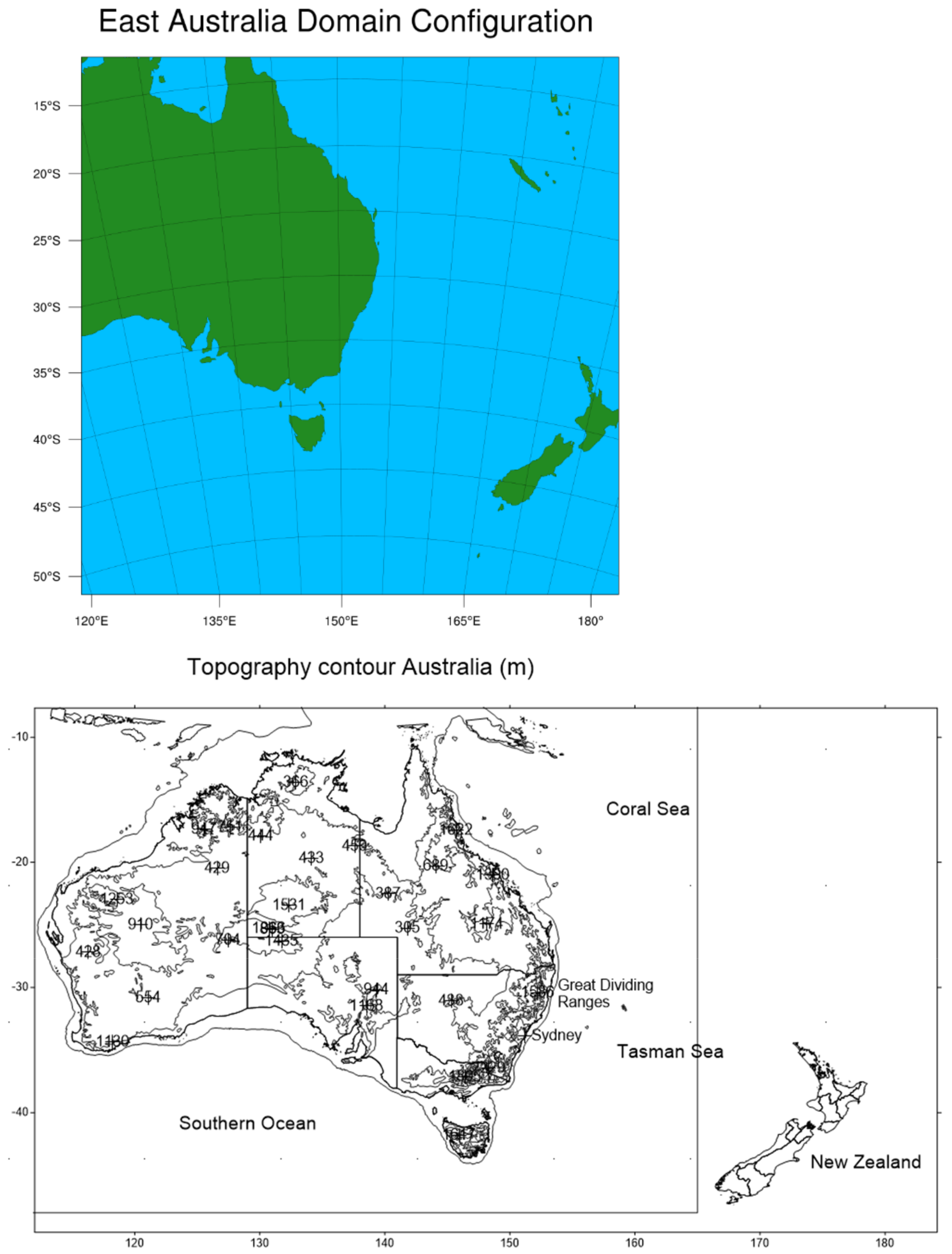As the Fe content in the soil or vegetation at the sources is dependent on the type of soil or vegetation, we assume that the amount of Fe traces when transported to the receptors is proportional to the amount of PM_2.5 and PM₁₀ emitted at the sources. The deposition velocity is used to estimate the particle flux to the ground. The domain configuration and the physics/chemistry options in the WRF-Chem model for this study are given in Figure 1 and

Table 1. WRF-Chem model physics and chemistry parametrisation.

WRF-Chem Physical Parametrisation	Namelist Variable	Option	Model/Scheme
Microphysics	mp_physics	3	WRF Single Moment
Land surface	sf_surface_physics	2	Unified Noah Land-Surface Model
Surface layer physics	sf_sfclay_physics	1	Monin–Obukhov similarity
Planetary Boundary Layer	bl_pbl_physics	1	Yonsei University Scheme (YSU)
Shortwave radiation	ra_sw_physics	4	Rapid Radiative Transfer Model for GCM (RRTMG)
Long wave radiation	ra_lw_physics	4	Rapid Radiative Transfer Model for GCM (RRTMG)
Cloud cumulus	cu_physics	1	Kain–Fritsch Scheme
Chemistry mechanism	chem_op	112	MOZART/GOCART chemistry/aerosol scheme
Dust emission	dust_opt	3	GOCART/AFWA dust emission
Photolysis	phot_opt	3	Madronich F-TUV photolysis
Gas dry deposition	gas_drydep_opt	1	Include dry deposition of gas species
Aerosol dry deposition	aer_drydep_opt	1	Include dry deposition of aerosols
Sea salt emission	seas_opt	1	GOCART sea salt emission
Biomass burning emission	biomass_burn_opt	2	Include biomass burning emissions and plume rise calculation for MOCART
Aerosol radiation feedback	aer_ra_feedback	1	Include feedback from the aerosols to the radiation schemes
Aerosol optical property	aer_op_opt	2	Aerosol optical properties calculated based upon Maxwell approximation

.

The domain grid size is 386 × 386 with a grid resolution of 12 km × 12 km in Lambert projection. The centre reference coordinates are ref_lat = −33.921 and ref_lon = 150.944. The domain contains the eastern part of Australia with the Great Dividing Range along the coast from the state of Victoria in the south to New South Wales and Queensland in the north. This mountain range divides the climate into 2 distinct regions. The coastal areas have more rain and are wetter, while the western sides of the mountain range are drier further inland into the desert areas of central Australia. The climate is varying from north to south with a tropical climate in northern Queensland; subtropical climate in southern Queensland and northern New South Wales (NSW); and temperate and oceanic climate in NSW and Victoria. The main climate drivers are the El Niño Southern Oscillation (ENSO) in the Pacific Ocean, the Indian Ocean Dipole (IOD) in the Indian Ocean and the Southern Annular Mode (SAM) in the Southern Ocean.

To associate the increase in the PM_2.5 deposition rate from dust and fire events with the increase in phytoplankton growth, spatial patterns of PM_2.5 deposition rate over the ocean are compared with observed phytoplankton patterns. Time series of the predicted PM_2.5 deposition rate at some selected points in the ocean will also be compared with the phytoplankton concentration. In this way, both spatial and temporal PM_2.5 prediction from the model will be compared or correlated with observed phytoplankton data.

3. Results

3.1. Dust Storm of 12–16 February 2019

Remote sensing data from polar-orbited MODIS Aqua/Terra satellites and the geostationary Himawari satellite before and after the dust storm event provide observation on the chlorophyll-a concentration in the Tasman Sea between Australia and New Zealand, which is used to correlate it with the dust deposition patterns. The dust storm of 12 to 16 February 2019 originated in desert areas of Lake Eyre in central Australia on 11 February 2019. The dust cloud reached the eastern coast of Australia in the state of NSW on the 12th of February and lasted until the 14th of February in the Tasman Sea. Afterward, it subsided as the dust was transported to New Zealand. Air quality monitoring stations on NZ South Island detected a high PM_2.5 concentration when the dust intruded to the ground level as it travelled further south to Antarctica and the South Pacific [17].

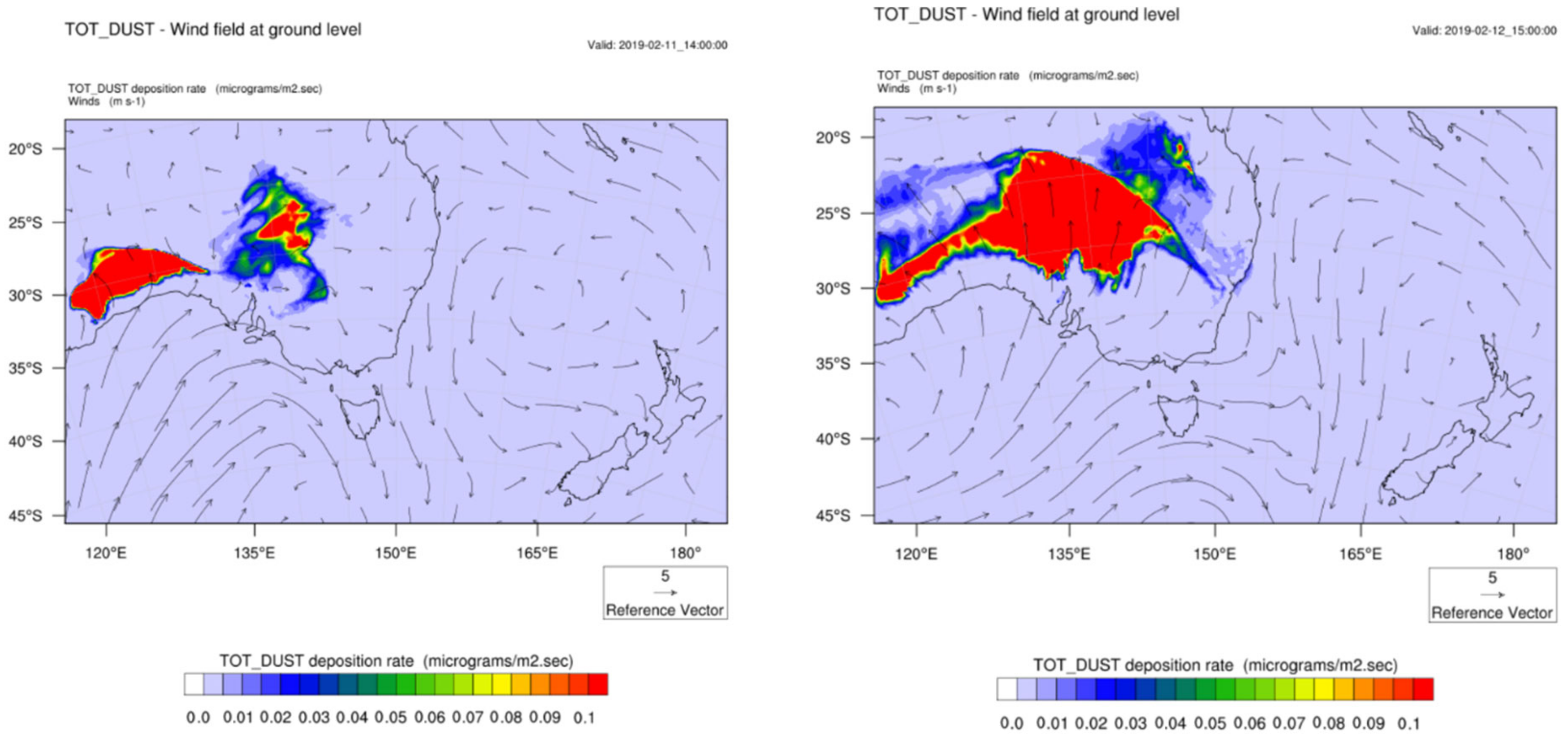
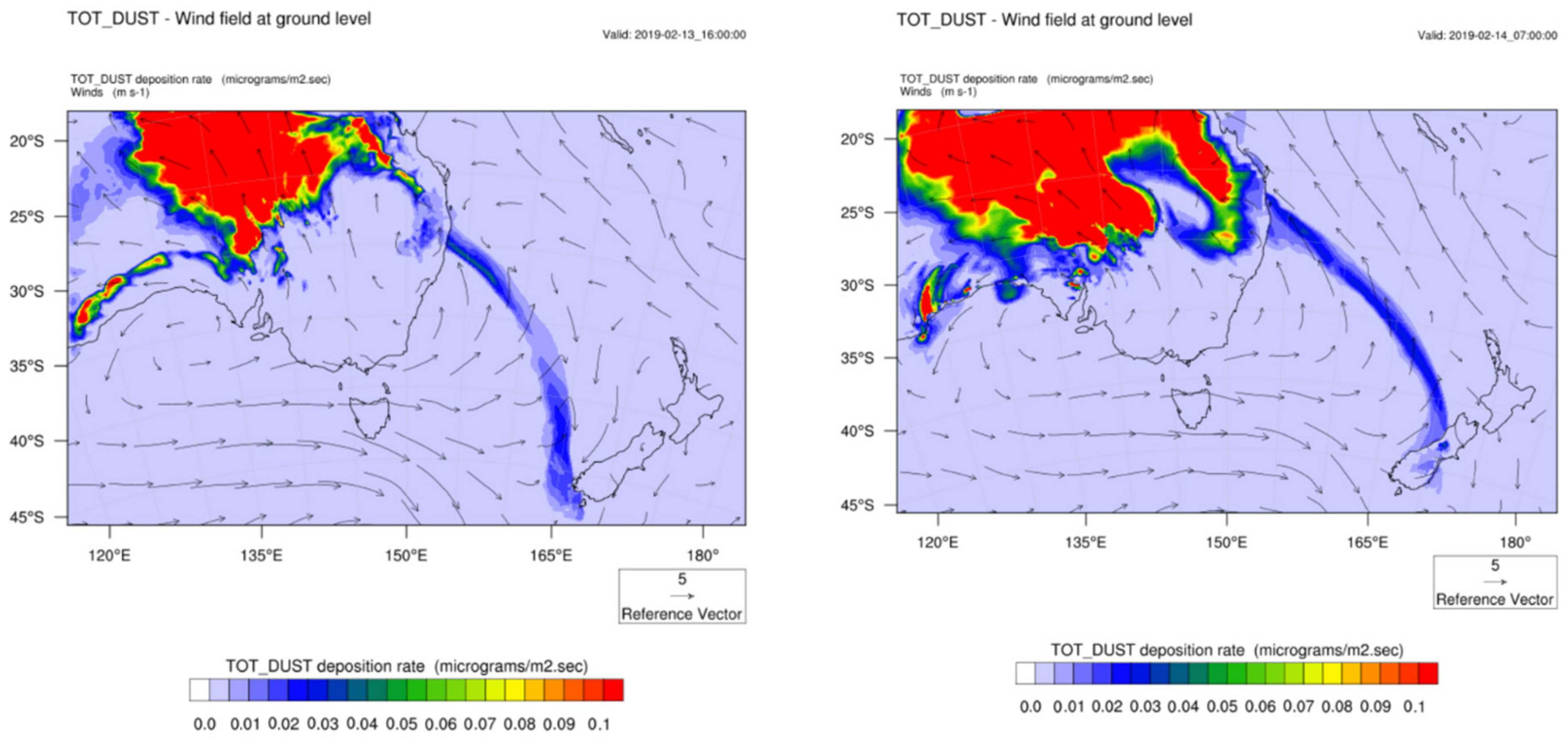
The progress of the dust storm from the sources in central Australia, western New South Wales and the east coast of Australia across the Tasman Sea to New Zealand and Antarctica was analysed in detail by [17]. Appendix A shows the simulation results of the dust storm progress from central Australia to the Tasman Sea with an overlaying wind field. The majority of the dust was transported to the north of Australia and Western Australia, while some dust was also transported to the east coast of Australia and the Tasman Sea. In the Southern Ocean, most of the observed AOD (Aerosol Optical Depth) was due to sea salt aerosols.

It has been shown by [17] that the dust, in this February 2019 dust storm, was able to be transported far from the sources to the Tasman Sea, New Zealand and Antarctica because of the presence of the Great Dividing Range along the south-eastern coast of Australia. The westerly wind carrying dust from the sources, west of the mountain range, crossed the mountain range and hence brought the airborne dust high above the troposphere. This high-altitude dust was then transported beyond the Australian mainland to New Zealand and beyond. The role of the Great Dividing Range as a launch pad for wind-born dust on its western side is important in the long-range transport of Australian dust during the dust storms.

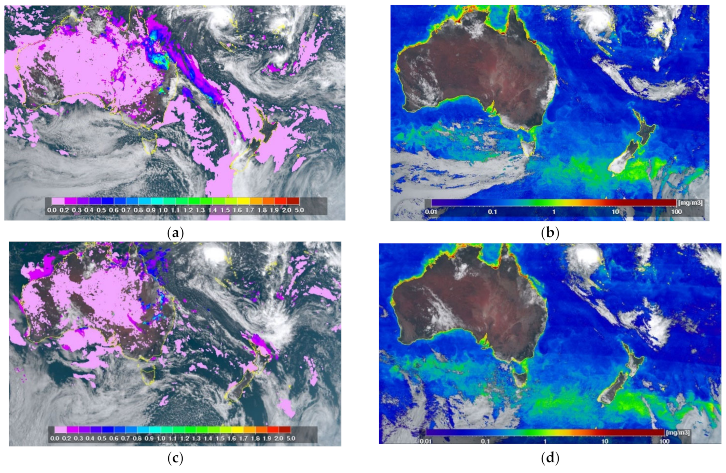
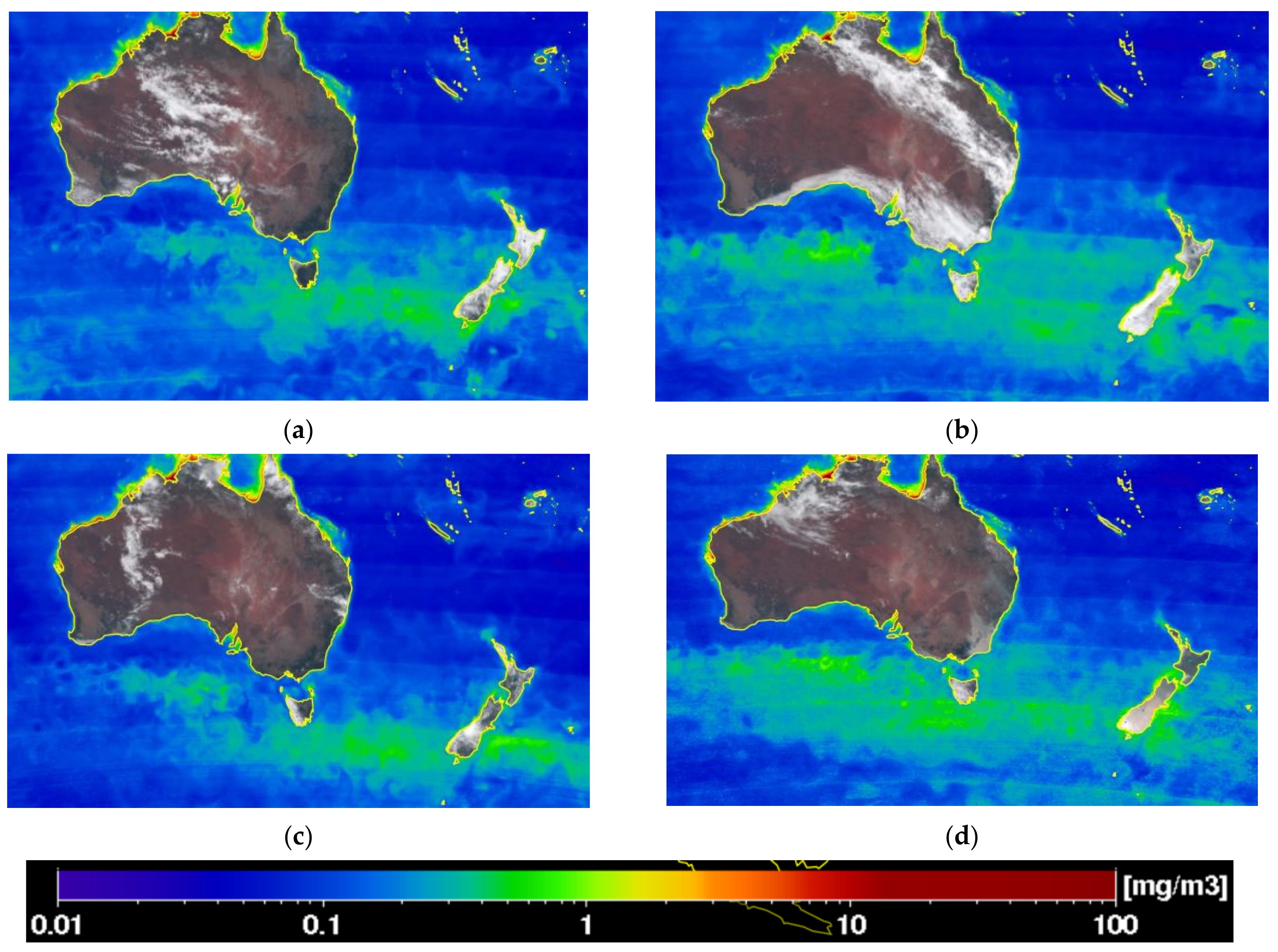
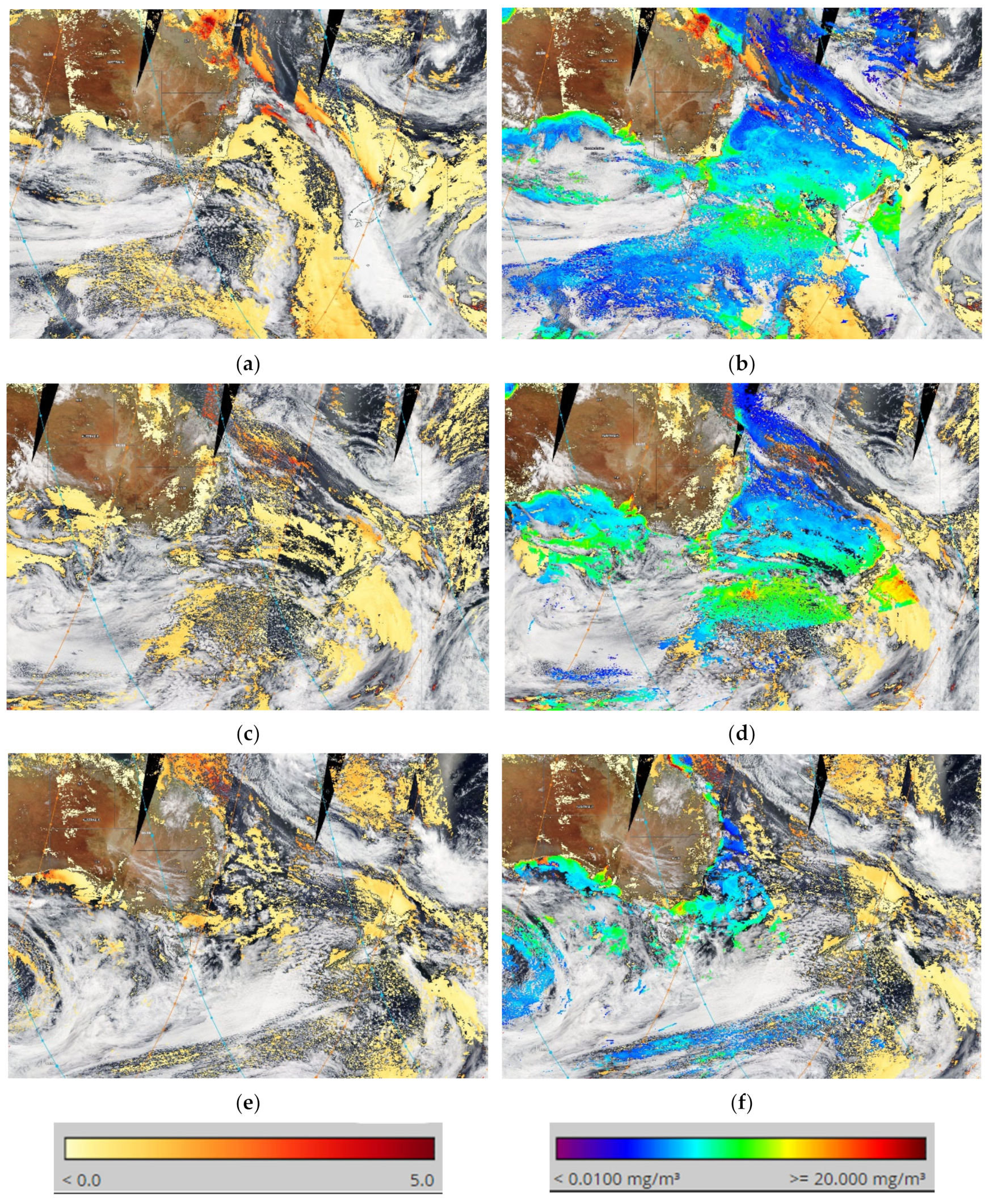
Figure 2 shows the AOD and chlorophyll-a over Australia during the dust storm from 12 to 16 February 2019 as detected by MODIS Terra/Aqua satellites. The sensors onboard the Himawari geostationary satellite also provided the real-time chlorophyll-a concentration over the Pacific Ocean from Japan to Australia. The Himawari processed data from JAXA (Japan Aerospace Exploration Agency) are at temporal resolutions of 10 min, 1 h, daily and monthly and are more detailed than those from the polar orbital MODIS Aqua/Terra satellites. 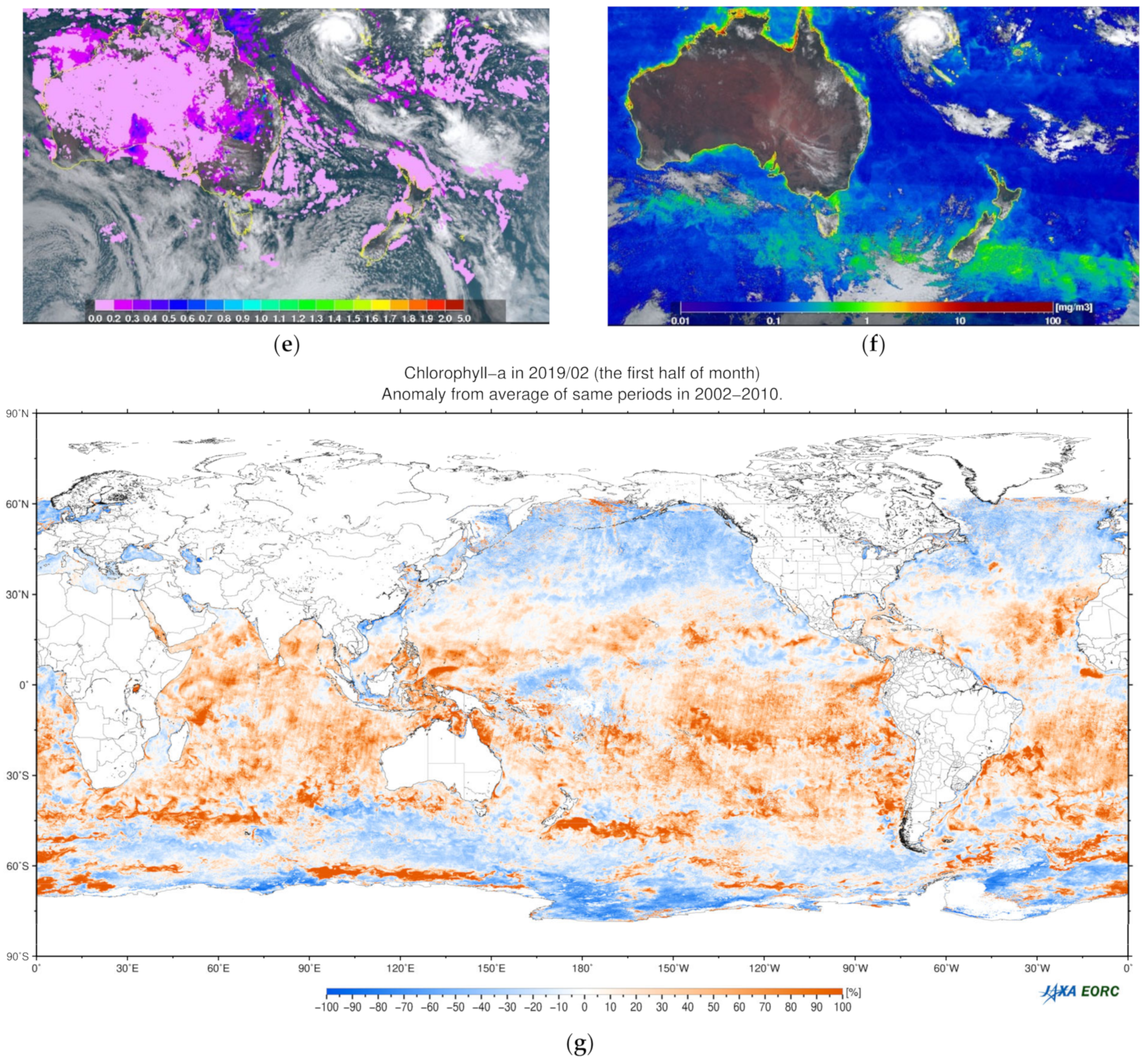Figure A2 in Appendix B shows the AOD and chlorophyll-a concentration as detected by the Himawari geostationary satellite on 14, 15 and 16 February 2019. Also shown in Figure A2g is the anomaly of the chlorophyll-a concentration in the first half of February 2019 after the dust storm compared to the average period of 2002–2010. The AOD and chlorophyll-a data products from both NASA and JAXA correspond well with each other.

As the phytoplankton growth only occurred after the dust deposition on the ocean under favourable conditions, the change in chlorophyll-a concentration in February 2019 as compared to the previous years (2002–2010) at a similar time was obtained as an anomaly map, which is shown in Figure A2g. Note that the biomass burnings and forest fires in Indonesia, the South East Asia mainland and South America during this period also contributed to the growth of phytoplankton in the Indian Ocean and Pacific Ocean.

The daily chlorophyll-a data at a 1 km resolution from the ESA Ocean Colour database for the period of 11 to 15 February 2019 were obtained and analysed for the spatial domain between lat [−24,−50] and lon [142, 179.9] encompassing the whole Tasman Sea, as shown in Figure 3. This domain covers the whole Tasman Sea. The mean chlor-a concentration varies from 0 to 0.5 μg/m³ in the Tasman Sea between the southeast coast of Australia and New Zealand. Below the latitude of −45° S, the high concentration of chlorophyll-a was due to phytoplankton growth in the Southern Ocean and was not connected to the partial dust-related phytoplankton growth in the Tasman Sea above. This can be seen in the spatial plot of the difference in the daily chlorophyll-a concentration and the previous daily concentration for each day on 12, 13 and 14 February 2019. This daily difference plot represents the new growth of phytoplankton for this day or an increase in chlorophyll-a concentrations as compared to the previous day. As the days progressed, the pattern of the new phytoplankton growth moved from the south-west to the north-east direction.

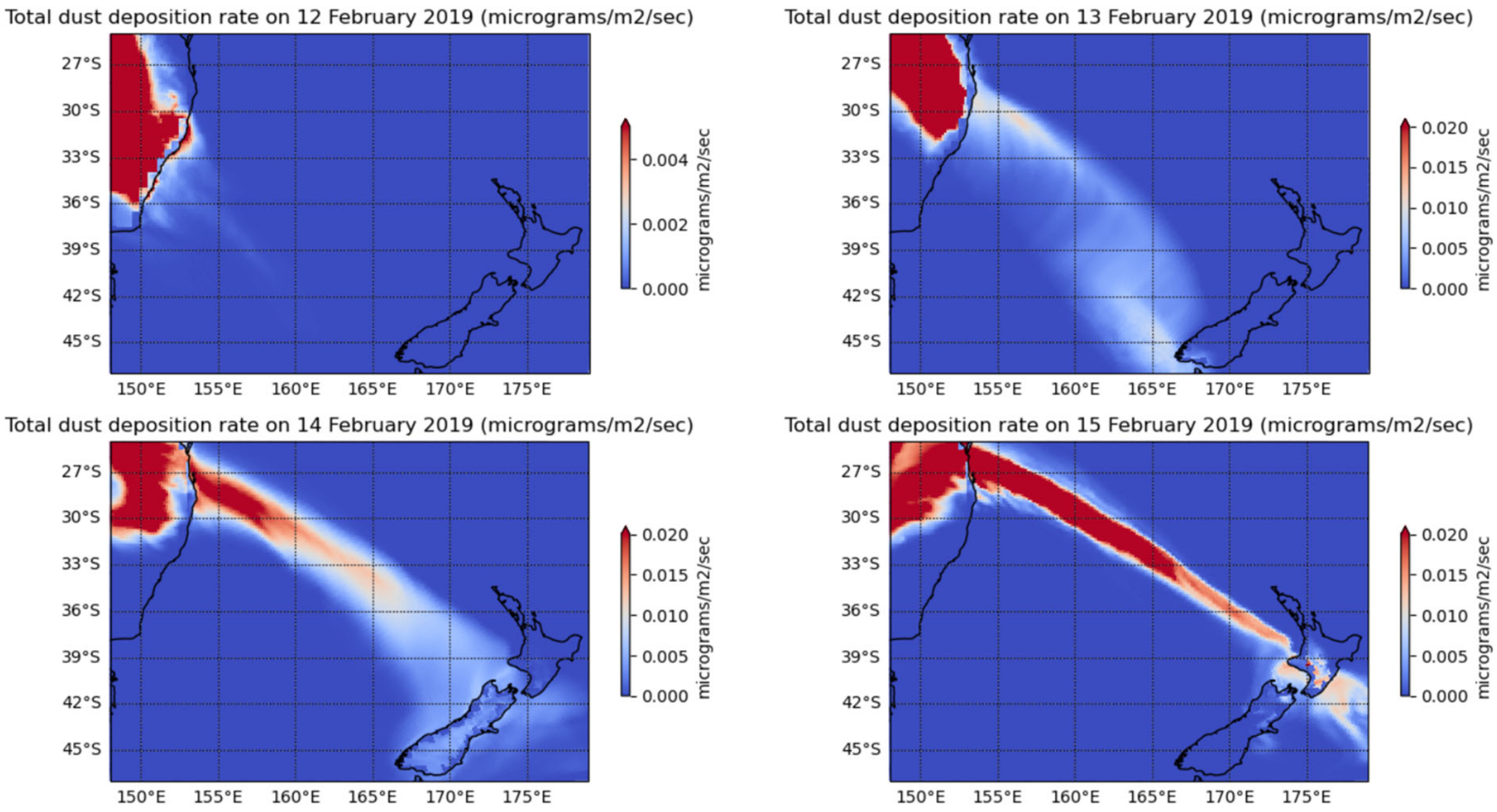
The WRF-Chem model simulation results of the deposition rate of total dust of different sizes (0.2–20 μm) each day from 12 to 15 February are shown in Figure 4. The dust deposition pattern gradually moved from south-west to north-east, which corresponds to the patterns of the chlorophyll-a growth or phytoplankton growth.

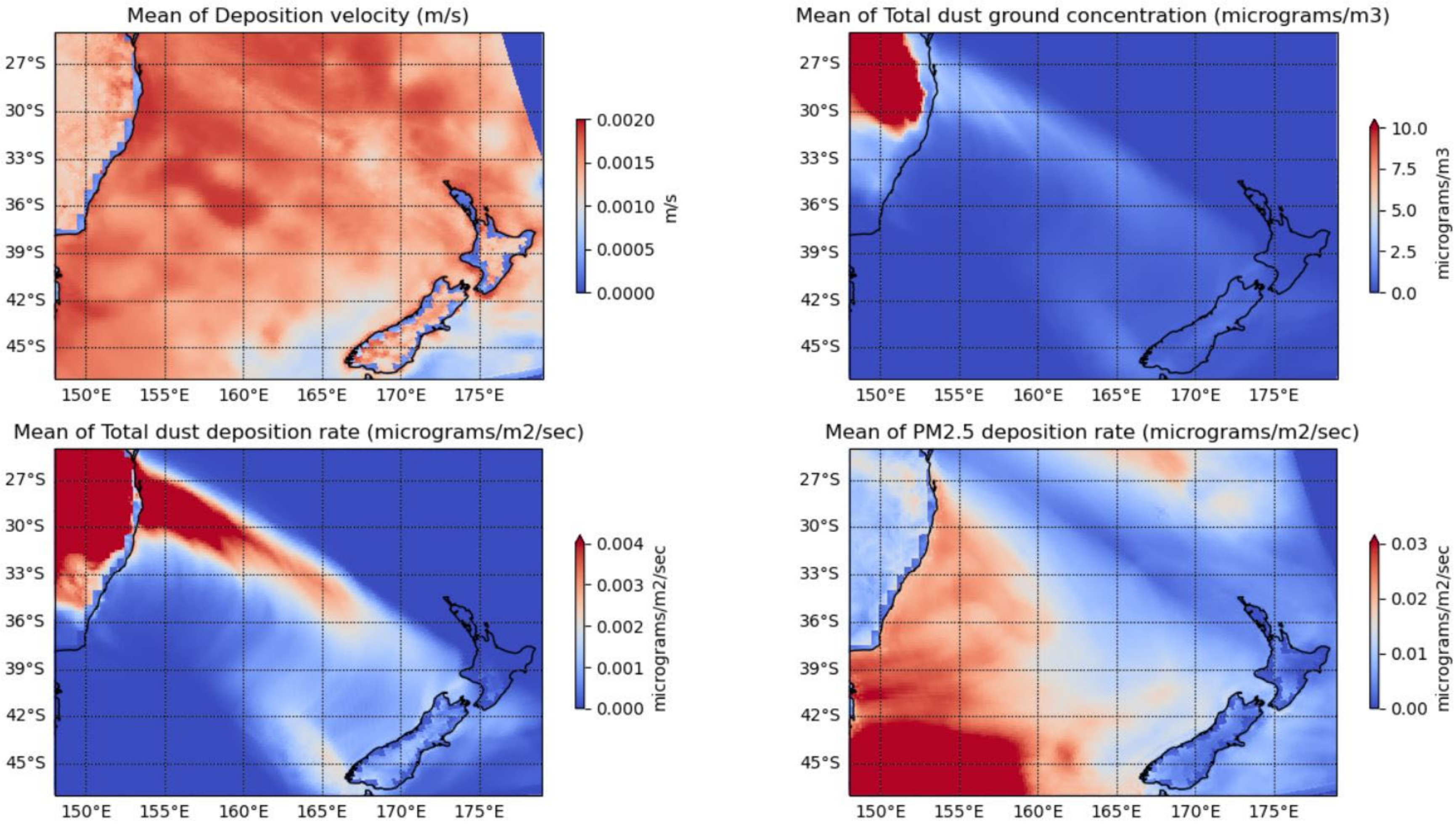
The results of the simulation of the WRF-Chem 4.1 model for the period of 11 to 15 February 2019 provide the spatial extent and the amount of dust particle deposition over the domain. Figure 5 summarises the results of the deposition of the total dust and PM_2.5 over the domain during the period of simulation. The mean deposition rate is obtained by averaging over the simulation period of the result of the multiplication of the deposition velocity and ground concentration of total dust or PM_2.5.

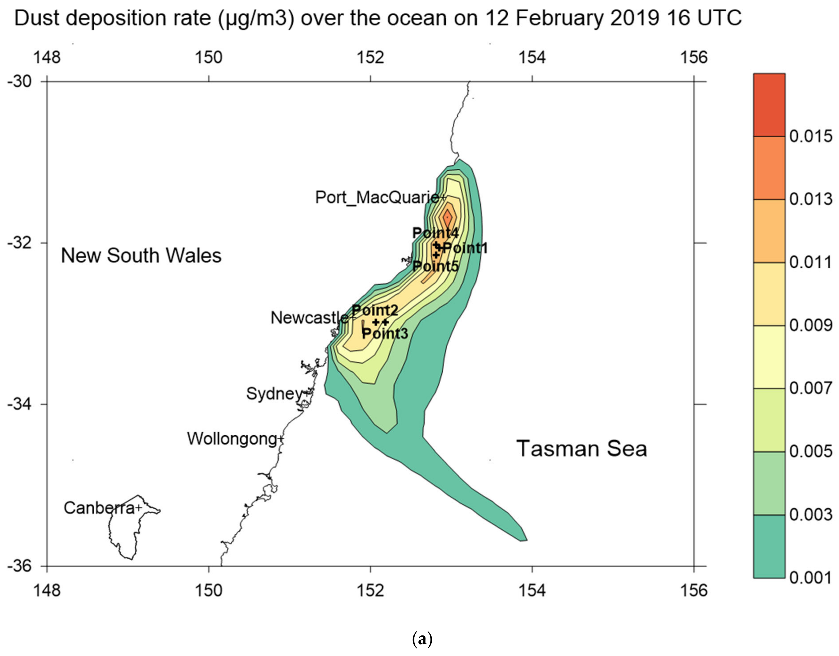
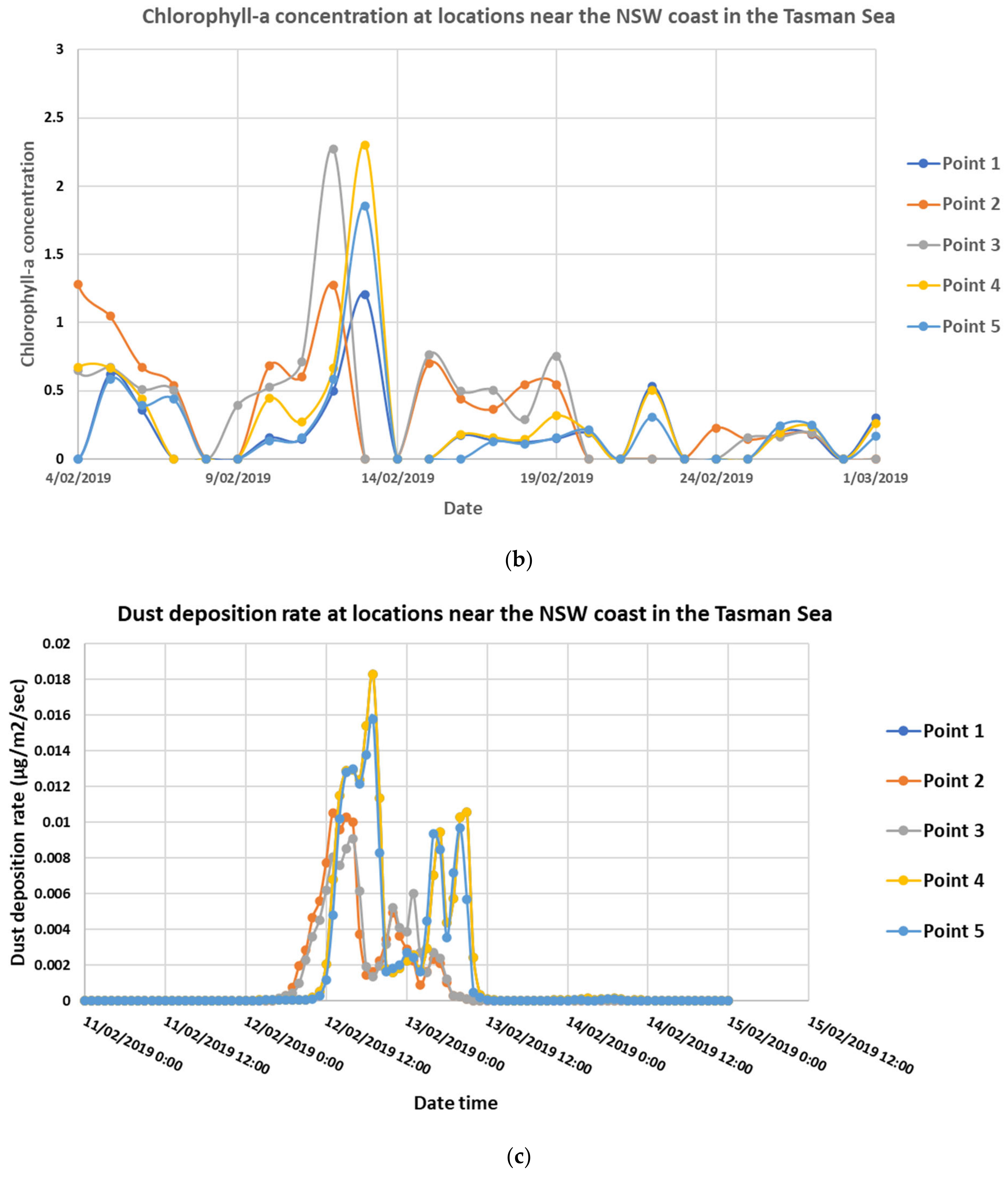
Time series of the chlorophyll-a concentration at some points near the coast where a high deposition of dust occurred are available. Shaw et al. 2008 [36] in their study of the effect of dust deposition from the 23 October 2002 dust storm on phytoplankton growth in Queensland coastal waters found that the high deposition of dust corresponds to days when the chlorophyll-a concentration is high. We also found that at a point location near the NSW coast where a high deposition rate occurred on the 12 and 13 February 2019, the chlorophyll-a concentration was also high, as shown in Figure 6.

Masking out the land mass feature, the estimated dust deposition in the Tasman Sea from WRF-Chem model simulation was calculated to be approximately 1230 tons of dust for 3 days from 12 to 15 February 2019 when the dust reached the Tasman Sea. The figure for dust deposition on land in the Australian simulation domain was about 135,000 tons, which is about 10 times higher than that on the Tasman Sea. The estimated accumulated total dust emission from central Australia from 11 to 15 February 2019 was approximately 2.4 million tons of soil dust.

3.2. Wildfire Event, Black Summer 2019–2020 Wildfires

The simulation of the early stage of the Black Summer 2019–2020 wildfire event from 1 to 8 November 2019 was also performed using the WRF-Chem air quality model to determine the emission and transport of pollutants and their effects on the environment, including the air quality in the atmosphere and in the marine system. In terms of the effect on greenhouse emissions, wildfires have more impact than dust storms as they emit a large amount of CO₂ into the atmosphere.

Van der Velde et al. 2021 [28] have estimated the amount of CO₂ emission in the Australian Black Summer wildfires to be 715 teragrams (range 517–867 trillion g) from November 2019 to January 2020 based on five different fire emission inventories: Global Fire Emission Database version 4s (GFED4s), the Fire Inventory from NCAR version 1.5 (FINN), Global Fire Assimilation System version 1.2 (GFAS), Quick Fire Emissions Dataset version 2.4 (QFED) and Fire Energetics and Emission Research version 1.0 (FEER). The estimations were then constrained by CO measurement from the TROPOspheric Monitoring Instrument (TROPOMI5) satellite. The CO₂ emission of the 2019–2020 wildfires surpassed Australia’s normal annual fire and fossil-fuel emissions by 80%. In their study of the effect of the 2019–2020 wildfires on phytoplankton growth, Tang et al. 2021 [19] identified a strong association of the AOD from this wildfire event above the Southern Ocean, south of Australia, and above the Pacific Southern Ocean (between New Zealand and South America) with the chlorophyll-a concentration in those ocean areas.

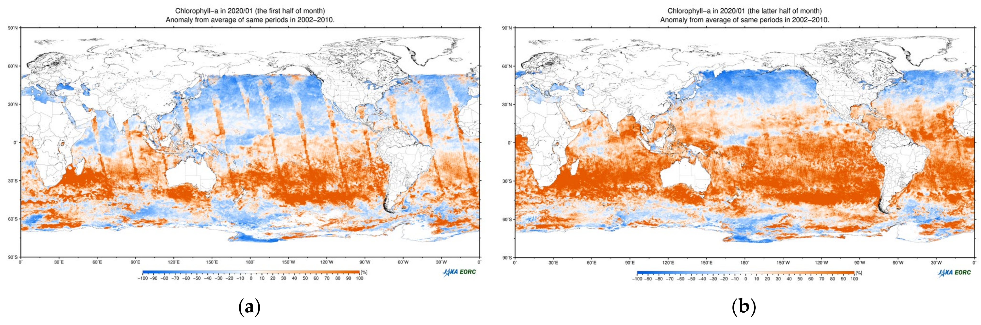
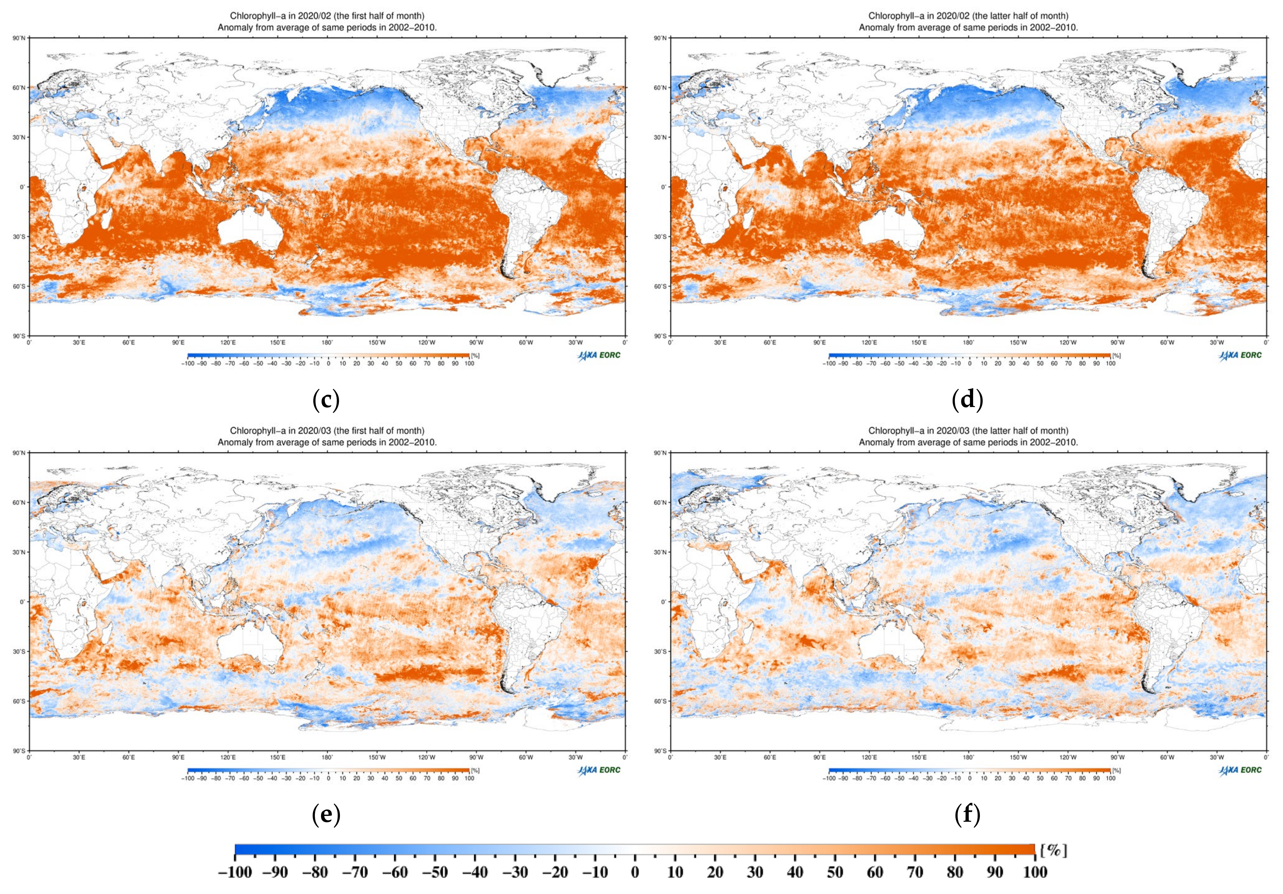
Figure A3 in Appendix C shows the monthly average chlorophyll-a concentrations as detected by a Himawari sensor in December 2019 and January 2020 as compared with those of the previous year. Note that the Himawari geostationary satellite does not cover the region beyond east of New Zealand near the International Date Line. A relative increase in the chlorophyll-a concentration can be seen in the Tasman Sea and Southern Ocean south of Australia. However, a clearer indication of phytoplankton blooms is shown by plotting the anomaly chlorophyll-a concentration across the southern hemisphere, including the Pacific part of the Southern Ocean, as shown in Figure 7. The images show massive phytoplankton growth from a high chlorophyll-a concentration over most of the water bodies in the southern hemisphere from Australia to South America and South Africa and back to Australia. This massive growth of phytoplankton lasted from January to early March 2010.

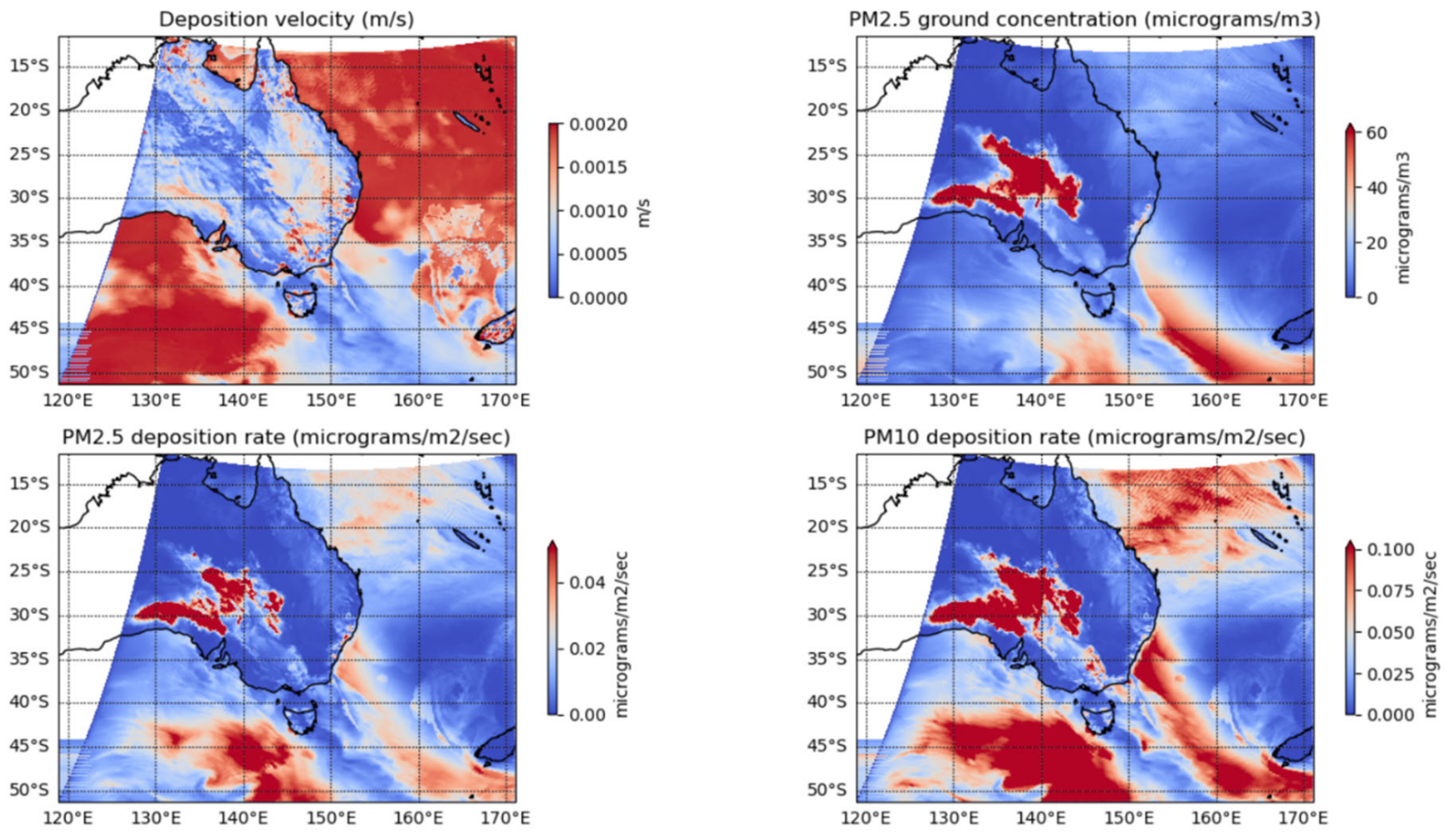
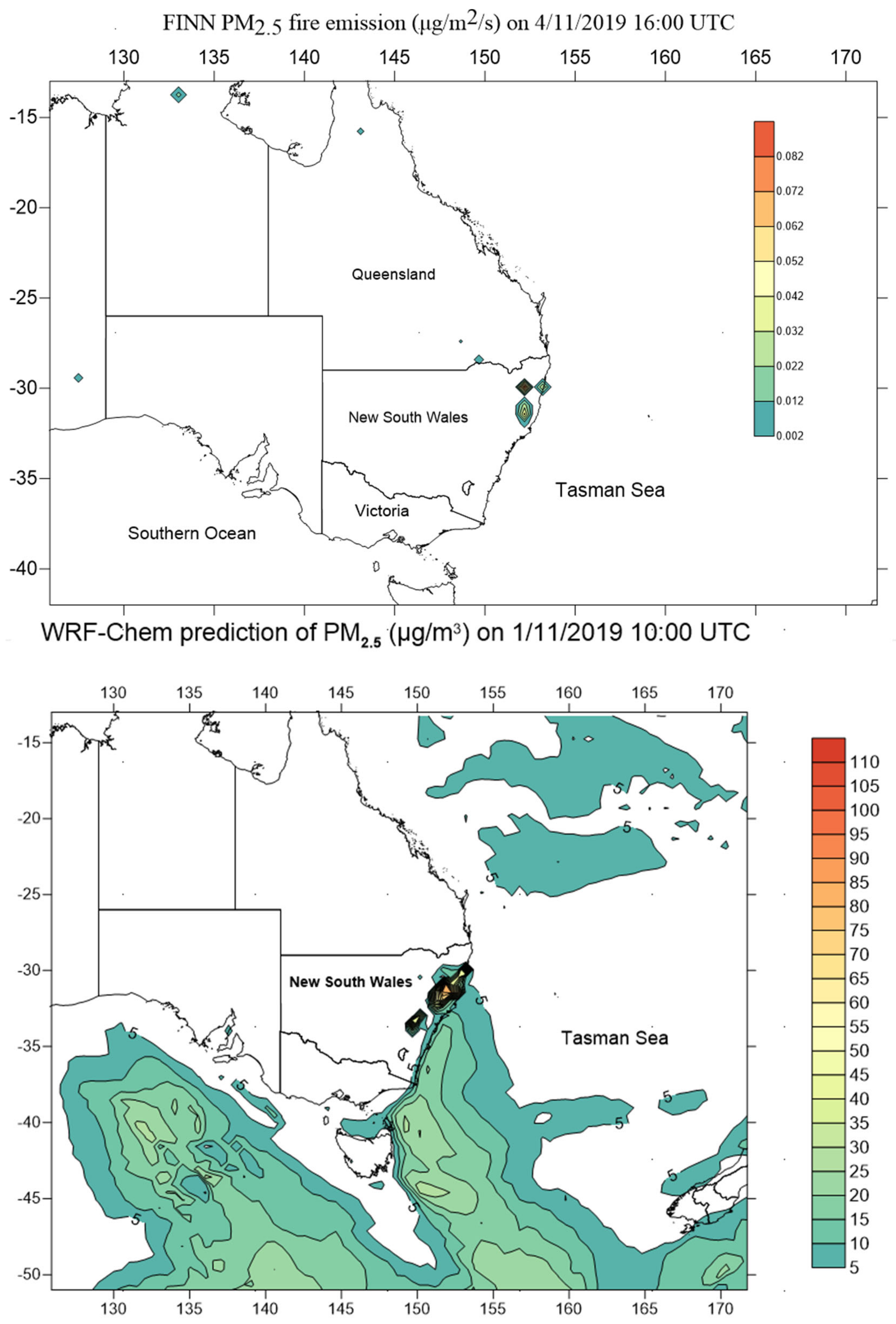
WRF-Chem model simulation in early November 2019, when the wildfires started, showed the transport of smoke aerosols and deposition of PM_2.5 and PM₁₀, which are shown in Figure 8 and Figure 9. The deposition on the Tasman Sea occurred due to smoke aerosols from the wildfires in northern NSW at this time. The major fires in the Blue Mountains in NSW, the border areas between NSW and Victoria, and the Gippsland areas of Victoria were not yet started until late November and December 2019.

The location of the fires in early November was in northern NSW and is shown in Figure 8 where the fire emission of pollutants was obtained from the FINN (Fire Emission Inventory from NCAR). These emission data are crucial in the simulation using an air quality model to predict the dispersion and concentration of pollutants at different levels in the atmosphere.

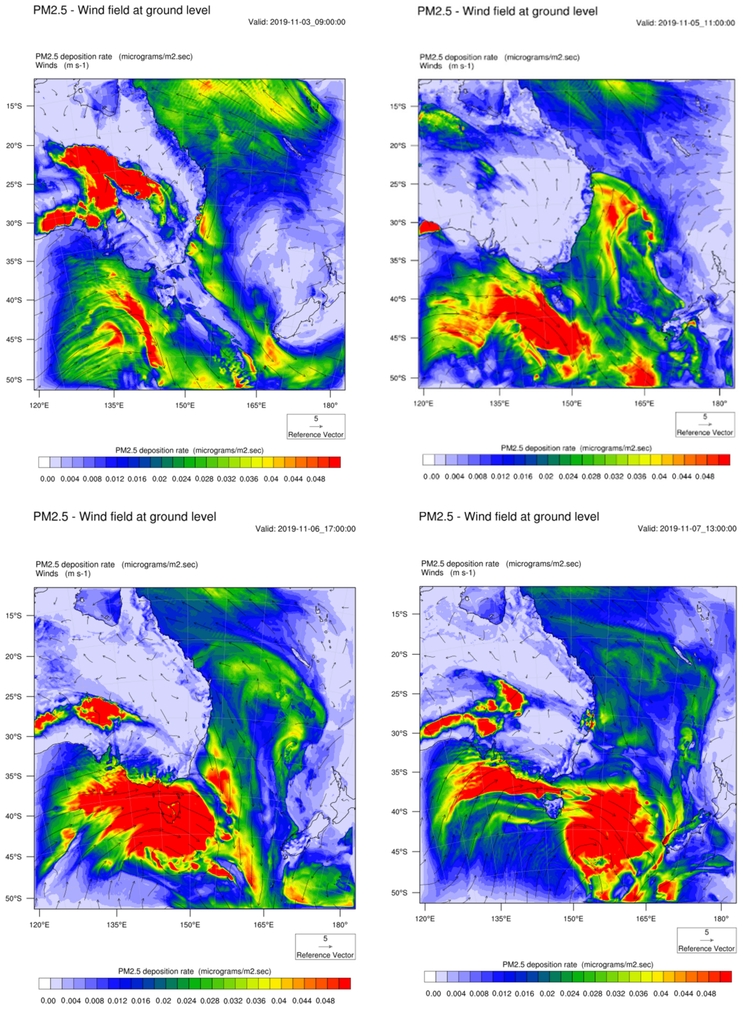
Figure 9 shows the predicted deposition velocity on 2 November 2019 was high in the Southern Ocean and in the Pacific Ocean, including the Coral Sea, north-east of Australia. But the ground concentration of PM_2.5 was low in those areas; therefore, the deposition rate of PM_2.5 was not dominant. In contrast, smoke aerosol plumes from the coast of northern NSW to the Tasman Sea and toward south of New Zealand in the Southern Ocean resulted in a higher deposition rate of PM_2.5 and PM₁₀ even though the deposition velocity was not high in the Tasman Sea.

Figure A4 in Appendix D shows the deposition rate of PM_2.5 and the wind field at ground level for the subsequent days (3, 5, 6 and 7 November 2019) at various times. The wind field shows a northerly wind pushed the smoke plume from the coast in the Tasman Sea to the Southern Ocean south of New Zealand. This smoke plume was then merged with a larger plume of sea salt PM_2.5 aerosols in the Southern Ocean.

Figure 9 and Figure A4 show the wildfires in northern NSW in early November resulted in a deposition of smoke aerosols of PM_2.5 and PM₁₀ from 1 to 7 November 2019 mostly in the Southern Ocean south of Tasmania and the Tasmania Sea between Australia and New Zealand.

Similarly to the dust storm analysis of chlorophyll-a, we used the ESA Ocean Colour daily chlorophyll-a data at a 1 km resolution for the period of 1 to 8 December 2019 to correlate with the predicted deposition rate from WRF-Chem model simulation. The spatial domain between lat [−24, −50] and lon [142, 179.9], covering the Tasman Sea, was used for the analysis. As chlorophyll-a data are only available at the highest temporal resolution on a daily basis, we aggregated hourly deposition data of PM₁₀ and PM_2.5 into daily data. As PM_2.5 and PM₁₀ predictions from the WRF-Chem model are similar in pattern, PM₁₀ data analysis is presented here. There are some difficulties in separating PM₁₀ from wildfires with other sources such as sea salt, which dominates its contribution to PM₁₀ in the Southern Ocean. Smoke aerosols and other pollutants from wildfires tend to disperse widely and much faster as compared with dust particles as the buoyant hot plume rise can penetrate the inversion layer in the troposphere. 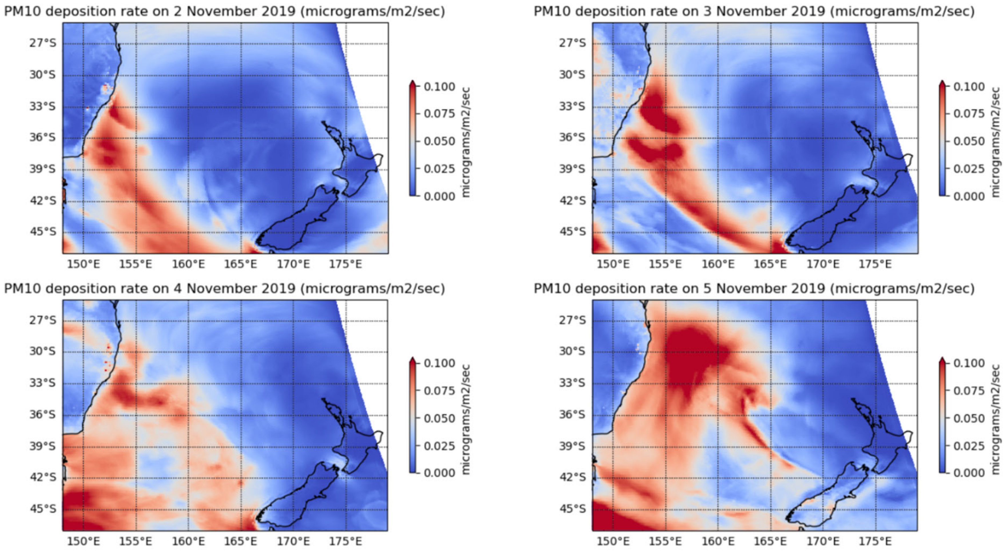Figure 10 and Figure 11 show the daily deposition rate of PM₁₀ and the distribution of the daily chlorophyll-a concentration in the Tasman Sea for 2, 3, 4 and 5 November 2019. The PM₁₀ deposition rate clearly shows the plumes of PM₁₀ extending from the coast of south-eastern Australia to New Zealand for these days.

There are some uncertainties in separating the PM₁₀ from wildfires and other sources (mainly sea salt emission from the ocean). The Southern Ocean emits a significant amount of sea salt as shown in the predicted PM₁₀ in this ocean south of the Australian continent and the Tasman Sea. This is different from the dust storm case. In the dust storm simulation, the total dust consisting of particles of different sizes (0.2–20 μm) is predicted separately from other sources so there is no ambiguity in assessing or correlating its impact on phytoplankton growth. 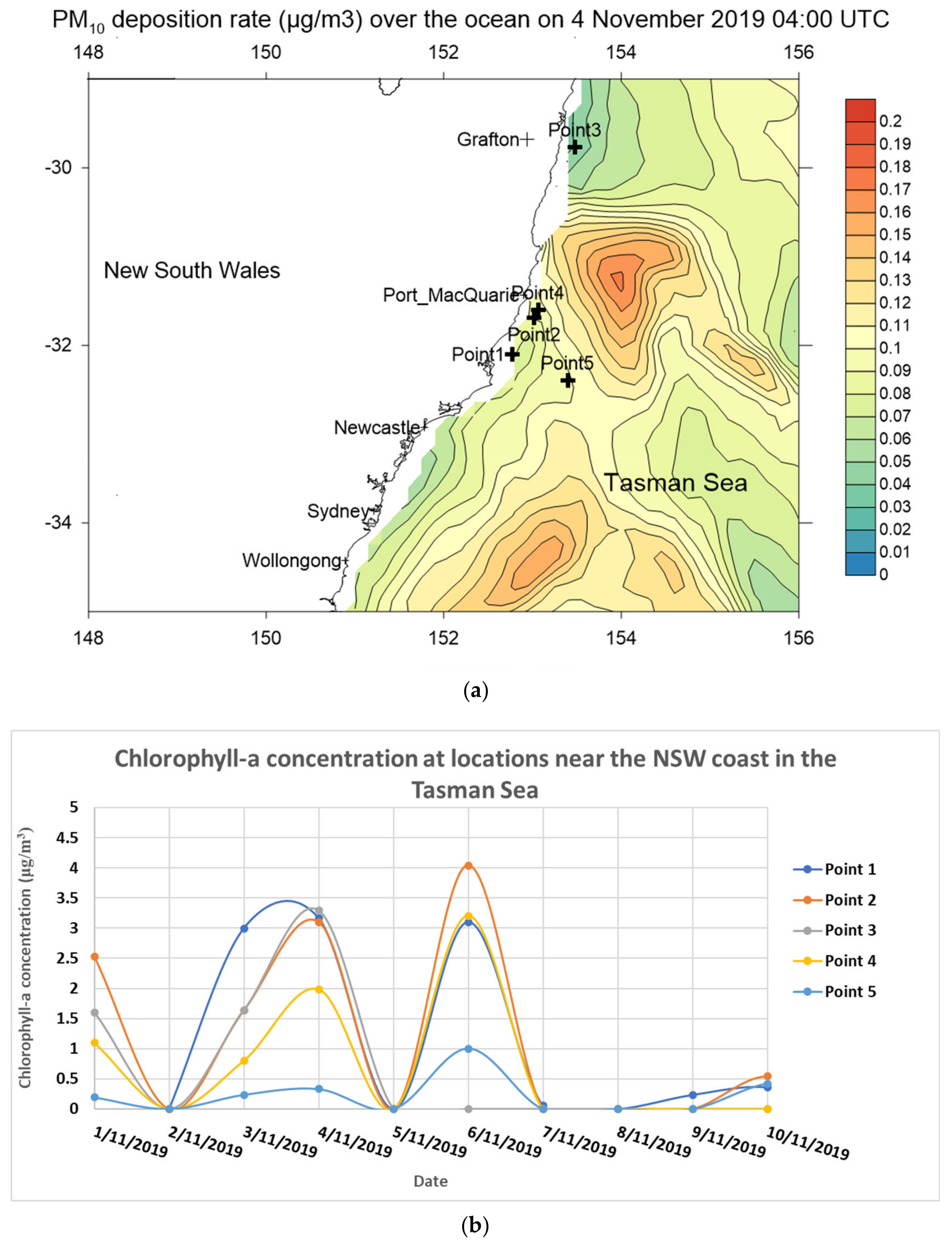The PM₁₀ plumes not far from wildfire sources allow one to be certain of their sources. Near the coast of New South Wales, close to the wildfire sources, a high concentration of chlorophyll-a was observed, as shown in Figure 12.

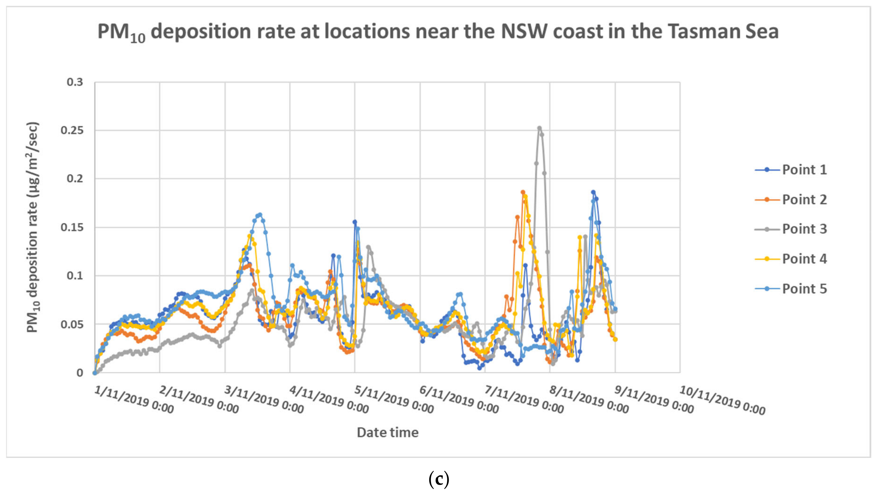
Figure 13 shows the time series of the chlorophyll-a daily concentration and PM10 deposition rate at five point locations in the sea off the coast of northern NSW. A high concentration of chlorophyll-a occurred on the 4 and 6 of November 2019, but time series (hourly) of the predicted PM₁₀ deposition rate at five point locations showed that high deposition rates occurred on 3 and 5 November 2019. On the 7 and 8 of November 2019, high PM₁₀ deposition rates occurred, but there were no chlorophyll-a measurements due to the cloud coverage of the area.

Other air quality models such as WRF-CMAQ allow one to tag the sources and therefore can determine separately their contribution to the total load of the predicted pollutant concentration. However, WRF-CMAQ is more complex to use in this mode and requires extensive computing resources. Another source of uncertainty in assessing the association of particulate matter deposition, such as some aerosols in the ocean, with phytoplankton growth is that the growth of phytoplankton also depends on a number of factors, such as the macronutrient levels, seasonal timing, light condition and initial state of the water ecosystem [19].

From the WRF-Chem model simulation, the total depositions of PM₁₀ and PM_2.5 in the Tasman Sea for the period of 1 to 8 November 2019 (the first stage of the Black Summer wildfires of 2019–2020) were approximately 132,000 tons and 45,400 tons, respectively. For deposition on land, the figures were 151,000 tons and 34,000 tons, respectively.

3.3. Comparision of the Dust Storm Impact and the Wildfire Impact on Phytoplankton Growth

The WRF-Chem model was used with the AFWA-GOCART dust emission scheme for the dust storm, while the same model configuration but with the MOZART chemistry mechanism and FINN (Fire Emission Inventory for NCAR) emission was used for wildfire simulation. For the Black Summer megafires lasting from November 2019 to January 2020, the peak of phytoplankton blooms occurred from January to early March 2020 when the deposition of smoke aerosols on the ground from aerosols above in the troposphere and in higher layers happened after they were being transported higher and farther away from the sources. After this time, from March, the growth disappeared, indicating that some of the carbon emitted by the megafires was reabsorbed by the ocean.

In comparison with the effect of the February 2019 dust storm on phytoplankton growth shown in Figure A2g, the dust storm emitted much less carbon and its effect on phytoplankton growth was via the iron (Fe) content in the dust. Australian soil is rich in iron compared to other countries, and from space Australia looks red in Western Australia and central Australia. The iron oxide minerology in soil is usually hematite (Fe₂O₃, 70% Fe), giving a reddish colour, or goethite (Fe₂O₃-H₂O, 63% Fe) with a yellow hue. In Australia, soil with strong hematite is located in most of Western Australia and central Australia, which is the source of many dust storms occurring in the east coast, while goethite soil covers most of northern and east coasts of Australia [37,38]. Soils taken from dust source regions in Australia were found to have ~3.5% Fe w/w (or 35,000 ppm) [39]. From these observations, it can be inferred that the dust storms typically contribute to the net carbon uptake and export carbon to the deeper layers of the ocean, acting as a sink. Conversely, wildfires emit carbon to the atmosphere, some of which is reabsorbed by vegetation on land and phytoplankton in the ocean. Wildfire events cause carbon loss to the atmosphere or are at best carbon neutral when reabsorption by biomass on land and ocean occurs. As predicted from the WRF-Chem model, the amount of PM₁₀ aerosols deposited in the Tasman Sea for the period of 1 to 8 November 2019 from the wildfires (132,000 tons) was much larger than that of the total dust deposition (1230 tons) due to the dust storm from 11 to 15 February 2019. Other aspects to consider are the Fe content in soil and vegetation. The Fe content in soil varies depending on the soil type and geographic location, while the Fe content in plants varies across different species and plant parts (after the root, the leaf has the second-highest Fe concentration). In a systematic review of Fe contents in plants, Ancuceanu et al. 2015 [40] have estimated the mean Fe content in leaves to be 489.4 (401.8–618.4) (ppm or mg/kg) based on data from 632 plant species.

To quantify the relationship between the frequency or amount of emission from dust storms and wildfires and phytoplankton growth, the use of modelling tools such as the WRF-Chem model is one method to use to predict the emission, dispersion and transport of pollutants to the receptors. This approach is adopted in this study.

3.4. Discussion

In this paper, a comparison study of the effect of dust storms and wildfires on phytoplankton growth in the Tasman Sea and Southern Ocean was conducted, investigating the 14 to 16 February 2019 dust storm and the first stage (1–8 November 2019) of the Black Summer megafires (November 2019–January 2020) as case studies. Both events promoted phytoplankton growth, but the megafires triggered a massive growth all around the southern hemisphere. The difference can be attributed to two factors: firstly, the megafires were much bigger and longer, and, secondly, the emitted carbonaceous nutrients from the fires deposited on the water surface can promote stronger growth. The total emission of carbon from the megafires was estimated by various authors [28,31] to be ~0.7 Pg (petagrams C), which is about 5 times the total annual Australian anthropogenic emission. Figure 5 shows the anomaly of the chlorophyll-a concentration in January, February and March 2020 from the average of the same period in 2002–2010.

Our results on the quantitative relation between deposited dust or smoke aerosols and phytoplankton growth at various sampling points near the Australian coast in the Tasman Sea are similar to the results of the study by Shaw et al. 2008 [36] on the effect of dust deposition from the 23 October 2002 dust storm on phytoplankton growth in Queensland coastal waters.

Luo et al. 2020 [41] conducted a study similar to our study by using the WRF-Chem model to simulate the dust storm originating from the Taklimakan Desert from 12 to 17 March 2015, which transported dust to the subarctic North Pacific Ocean (SNPO). Satellite data from MODIS and CALIPSO provided AOD and vertical profiles of dust, and chlorophyll-a data were used to corroborate with dust deposition prediction from the WRF-Chem model. They concluded that dust deposition in the SNPO might lead to an increase in phytoplankton there because of the iron fertilisation effect.

The validation of the WRF-Chem model prediction for the February 2019 dust storm and the 2019–2020 wildfires was performed in our previous studies [17,20] on these events. The predicted results of meteorology and air quality (PM₁₀, PM_2.5) performed well when compared to the observation. Therefore, we can have confidence in the WRF-Chem model predicted PM₁₀ dust and smoke aerosol deposition rate in the Tasman Sea.

Bowman et al. 2020 [42] in their study of Australian forests and megafires have highlighted the risk of dwindling carbon stocks from more frequent fires due to climate change. The projected increase in the frequency of wildfires due to climate change alters what was a carbon neutral process of reabsorbing emitted carbon by the forests, and subsequently it cannot be achieved, with the result of the net loss of sequestered carbon to the atmosphere subsequently further promoting a warming climate. The increasing megafire frequency will reduce the recovery capacity of reabsorbing the emitted CO₂ from the eucalyptus forest even though such native eucalyptus forests are known to be resilient and highly adaptable to fire-induced environments on the dry Australian continent. It is assumed by many policy makers that rapid recovery by forest generation would therefore result in CO₂ emissions being reabsorbed and fixed in those carbon storage sites [37]. However, rapid climate change could have run-away positive feedback that will leave no time for forest recovery and CO₂ reabsorption due to the anticipated increase in the frequency and magnitude of wildfires in Australia. It was suggested by Vajda et al. 2020 [38] in their sedimentary study in the Sydney basin that the End-Permian mass extinction event (EPE) about 252 million years ago was due to deforestation, wildfires and flooding.

In the Bowman et al. 2020 [42] study of carbon emission from the 2019–2020 wildfires, they estimated that about 0.67 Pg (petagrams; 1 Pg is 10¹⁵ g) of carbon was emitted from the 2019–2020 wildfires. This can be compared with the global 2019 annual emission of fossil fuel and land use change (mainly deforestation) of about 9.9 Pg and 1.8 Pg of carbon, respectively [39]. Van der Velde et al. 2021 [28] subsequently estimated that about 0.715 Pg of carbon was emitted from this wildfires period from November 2019 to January 2020, exceeding Australia’s 2018 anthropogenic CO₂ emissions of 537.4 million tons (0.147 Pg C) [19]. The emission of carbon from these 2019–2020 wildfires was nearly 5 times the total annual Australian anthropogenic carbon emission.

However, the effect of wildfires, such as the megafires of 2019–2020, on promoting phytoplankton growth in the Southern Ocean can have the potential to offset the emitted CO₂ significantly. Tang et al. 2021 [19], showed that the satellite-estimated marine net primary production (NPP) and export production (EP) increased substantially during the 2019–2020 wildfire period compared with the monthly climatology. From October 2019 to April 2020, a cumulative net additional uptake of ~186 ± 90 Tg (teragrams or 10¹² g) of carbon was absorbed by phytoplankton blooms, which is equivalent to ~95 ± 46% of the CO₂ emission (~195 Tg C) from the 2019–2020 Australian wildfires. Even though their estimate of a 0.195 Pg carbon emission from the 2019–2020 wildfires is lower than those from Bowman et al. 2020 [42,43,44,45] (0.67 Pg) and from Van der Velde et al. 2021 [28] (0.715 Pg), the high proportion of carbon uptake by phytoplankton growth showed that most of the carbon emitted by the wildfires was absorbed via phytoplankton growth in the Southern Ocean.

As Tang et al. 2021 [19] noted in their study, not all bodies of oceanic water respond to Fe fertilisation by pyrogenic aerosols with strong phytoplankton growth as this also depends on the macronutrient levels, seasonal timing, light condition and initial state of the water ecosystem. Such is the case of oligotrophic subtropical waters east of Australia where the limit of the macronutrient level shows a lack of chlorophyll-a response.

As large wildfires occur less frequently compared to dust storms over the southern part of the Australian continent and the total Australian soil emission in terms of volume contains more Fe than that in the emission of biomass burnings, the phytoplankton bloom in the seas off the south-eastern Australian coast from dust is more significant. Our estimate of the amount of PM₁₀ deposited in the Tasman Sea during the dust storm of 11 to 15 February 2019 is 1230 tons. Assuming the content of Fe in the soil was ~3.5% [39], then the amount of Fe in the PM₁₀ deposited in the Tasman Sea was ~43 tons. In comparison with the wildfires during the initial burning period from 1 to 8 November 2019, the predicted amount of PM₁₀ deposited is ~132,000 tons. And assuming the Fe content in the leaves of all burned plant species is 490 ppm w/w, then the estimated Fe in the PM₁₀ deposited from the wildfires is ~65 tons. The figures for the deposited Fe in the Tasman Sea during the dust storm of February 2019 and for the initial stage (1 to 8 November 2019) of the wildfires are comparable. However, the wildfires lasted longer (to early January 2010), and smoke aerosols travelled beyond New Zealand to the Pacific Ocean and South America and back to Australia across the Indian Ocean where smoke aerosols were also deposited and promoted phytoplankton growth.

Even though the air quality model is a useful tool in estimating the dispersion, transport and deposition of pollutants from source emission, there are some uncertainties in the modelling results. Tan et al. 2019 in their study of the differences in the prediction of particulate matter (PM) among various models, including the WRF-CMAQ (v4.7.1 and v5.0.2), WRF-Chem (v3.6.1 and v3.7.1), GEOS-Chem, NHM27 Chem, NAQPMS and NU-WRF models, have found that the difference is mainly due to different natural emission mechanisms, such as dust and sea salt, initial and boundary conditions, the gas-particle conversion phase and different amounts of depositions.

Zhang et al. (2019) [46] compared the modelled dust deposition using the GOCART aerosol scheme in the WRF-Chem model with the observed dust deposition and found that the modelled dust deposition is highly underestimated by more than one order of magnitude compared to the observed deposition. This indicates that the dry deposition scheme [35] in the GOCART aerosol scheme may not be suitable for dust simulation and needs to be further improved. The Ginoux DSF used in the WRF-Chem model is a static function as it is based on topography. This can be modified to account for the changing land cover. Besides improving the DSF, other aspects of dust emission processes can be improved to characterise the emission over surface roughness, as demonstrated by [47], who proposed using albedo from satellites to better represent the shadow and sheltered area from dust mobilisation.

If both wildfire and dust storm events happen at the same time, such as when the dust storm event on the east coast of Australia in February 2019 and wildfires in northern NSW happened at the same time, then how do we separate the dust and fire carbon impacts? This is difficult to work out if both events happened at the same time, which could happen frequently in the future changing climate. Modelling is one of the answers in this case.

In this study, we have shown that there is strong evidence that the sequestration of CO₂ by an enhanced biological pump via phytoplankton growth occurred during the February 2019 dust storm and the Black Summer 2019/2019 wildfire events. But how long this sequestration is and what amount of carbon it would store in the ocean at different depths is not known and will be the subject for further study. This is important for policy makers wanting to account for the carbon absorbed and sequestered in the ocean to formulate a response to climate change.

4. Conclusions

In this study, we have chosen the 12–16 February 2019 dust storm and the megafires in November to January 2019–2020 for a comparison of phytoplankton growth in the Tasman Sea as case studies. We have shown that there is strong evidence from a simulation study that the growth in phytoplankton in the Tasman Sea in mid-February 2019 and in the early stage of the Black Summer wildfires (from 1 to 8 November 2019) was due to the dust deposition from the dust storm and the smoke aerosols from the wildfires, respectively. The amount of deposition of particulate matter from the wildfires is much larger than that of the dust storm. The WRF-Chem air quality model has been shown to be a useful tool to study and determine the pattern of impact of particulate matter on the phytoplankton growth in the Tasman Sea. We have shown that it is possible to quantitate the relationship between the emission and deposition of particulate matter (such as PM₁₀) and the subsequent phytoplankton growth in the receiving water bodies.

The phytoplankton growth absorbed CO₂ via photosynthesis and hence acted as a carbon sink. Both events promoted phytoplankton growth, but the megafires triggered a massive growth all around the southern hemisphere. The difference can be attributed to two factors: firstly, the megafires were much larger and longer, and, secondly, the emitted carbonaceous nutrients from the fires deposited on the water surface promoted stronger growth of phytoplankton.

The phytoplankton blooms occurred from December 2019 to early March 2020, shortly following the wildfire events. After that, the growth disappeared, which is largely attributed to CO₂ being reabsorbed by the ocean. How much of that carbon was sequestered at different depths in the Tasman Sea and Southern Ocean and for how long are not known and require further study. In addition to this, our future investigation will also be focussing on characterising source soil types, vegetation species and Fe contents to be incorporated into the emission input to the WRF-Chem model.