Full-Size Experimental Measurement of Combustion and Destruction Efficiency in Upstream Flares and the Implications for Control of Methane Emissions from Oil and Gas Production

Abstract

Accurately measuring the combustion and destruction removal efficiency of flaring is important when accounting for methane emissions from oil and gas production. Despite this, the amount of experimental data from full-size flares is limited, especially for flares built without air or steam assistance. The use of a single destruction value of 98% is commonly applied. In this paper, we present new empirical measurements of flare efficiency using three common flare designs employed in upstream applications. Combustion products were analyzed using an extractive sampling method. The results demonstrate that whilst destruction efficiencies in excess of 98% are achievable, if the gas composition falls below a critical heating value of ~300 BTU/scf, the efficiency deteriorates leading to elevated methane emissions. This is further complicated by accurately measuring the flow of combustible gas and the impact of crosswinds. In an operational setting, continuous tracking of flare conditions is therefore a key resource in reducing methane emissions but further work is required to standardize how continuous performance tracking is evaluated if such measurements are to attain full traceability.

1. Introduction

Methane (CH₄) is a potent but short-lived greenhouse gas with a global warming potential 28 times greater than CO₂ over a 100-year timescale, increasing to 84 times if considered over 20 years [1]. Since the industrial revolution, atmospheric methane concentrations have more than doubled, accounting for 25% of anthropogenic global warming [2]. However, unlike carbon dioxide, reductions in the rate at which methane is emitted could slow or reverse this trend [3]. There are numerous sources of anthropogenic methane, including enteric fermentation, rice production, agricultural and urban waste. Methane from oil and gas production and usage accounts for approximately a third of emissions [4]. As such, methane reductions from oil and gas production and use are widely seen as the most accessible opportunity for achieving reductions on these timescales [5].

Methane emissions from oil and gas production and use can occur throughout the value chain, but for many producers, one of the most significant sources is flaring. The World Bank estimates that over 138,000 million m³ of gas is flared globally each year [6]. Unlike some other key sources of emissions, such as fugitives, the flare is frequently an integral part of the design and safe operation of many existing oil and gas facilities. The World Bank recognizes three classes of flaring: routine flaring (used to optimize oil production where gas volumes exceed infrastructure capacity), non-routine flaring (including maintenance activity and well clean-up) and safety flaring (equipment malfunctions and plant blow-downs). Whilst initiatives, such as the World Bank zero-routine flaring by 2030 initiative, have led to measurable reductions in routine flaring, the need for flaring during maintenance and in emergency situations to keep workers safe means they shall continue to be part of some oil and gas production for the foreseeable future.

Methane is emitted to the atmosphere when flared gases do not fully combust. Quantifying flare combustion uses two closely related values: combustion efficiency and destruction and removal efficiency. Combustion efficiency (CE) is a measure of the conversion of hydrocarbons to CO₂, whereas destruction and removal efficiency (DE or DRE) also accounts for the incomplete combustion products of CO and soot [7]. DRE is used for calculating methane emissions for greenhouse gas reporting over CE as it includes all methane converted to intermediate combustion products.

Flares used in the oil and gas industry come in different sizes, designs and modes of operation. Some flares use steam or air introduced at the flare tip to aid combustion and inhibit visible soot formation. These are most encountered in the downstream (refinery) sector and referred to as assisted flares. By contrast, many upstream flares are normally operated without air or steam. These include both unassisted flares and pressure-assisted flares that use the flow of flare gas to maintain combustion. Flares also vary in size and design, including the use of inert gases such as nitrogen to stop the ingress of air into the flare stack under low flow conditions (purge gas). There is a wide variety of manufacturer-specific proprietary designs that moderate the flow of gas to facilitate turbulent mixing with the air as an aid to combustion. These include a range of fixed and variable restricted orifices that increase exit velocity and the use of multi-arm flare tips to disperse the gas over a wider area. The use of flare pilots is not ubiquitous, even though it is often critical to keep a flare lit especially under low flow conditions or where the flow contains a significant proportion of inert gases.

Many factors affect the CE/DRE of flares. Alongside the design of the flare, the gas composition and flow rate are key considerations [8]. Accurately measuring the flow rates in flares is complicated because of the large difference in flow between a flare that is at the minimum flow required to remain lit and avoid air ingress (often referred to as the purge rate) and during a full facility blow-down event in which all the gas in the production train must be safely evacuated. This turndown ratio in flow can be up to three orders of magnitude [9]. CE/DRE is further influenced by environmental factors, most notably crosswind speeds. At high-wind velocities, uncombusted gas can be ‘stripped’ from the combustion zone resulting in a lower CE [10,11].

There is a convention in the upstream oil and gas industry that 2% of methane is emitted to the atmosphere from upstream flares because of incomplete combustion, otherwise referred to as 98% DRE. In some countries, this value forms part of the regulated reporting of emissions [12]. The origins of the 98% DRE lie in research conducted in the early 1980s by the US Environmental Protection Agency (EPA) and later extended by the Texas Commission for Environmental Quality (TCEQ) [13,14,15] where the focus of the work was on assisted flares and the reduction of visible emissions of flaring, such as soot formation.

Recently, the 98% DRE figure has come under increasing scrutiny because of its significance in assessing greenhouse gas emissions. For example, airborne measurements taken from onshore US showed that DRE values range from below 70% to 100% [16]. In this setting, some flares were also unlit, and the gas was venting to the atmosphere. By contrast, measurements in the Norwegian sector of the North Sea demonstrated an average DRE of 98.4% [17]. As flaring is frequently one of the largest reported sources of methane, knowing the true DRE value matters for accurate reporting. At 99% DRE, the methane emission from flaring halves, or doubles at 96% (when compared to an assumed 98% value). Measuring the specific DRE value for a flare is therefore of critical importance if methane emissions are to be accurately tracked and used as the basis for effective emissions reduction strategies. This is recognized in a new generation of emergent initiatives and regulations including the UN-led Oil and Gas Methane Partnership 2.0 [18].

Measuring the CE/DRE of flares is difficult. In an operational setting, the flare is, by design, inaccessible as a safety precaution making direct sampling from the combustion plume untenable. Previous research has sought to extend the body of data by conducting scaled experiments in wind tunnels [11]. However, these are restricted in their capacity to replicate the design of the more complex flare tips. Field experiments using spectrographic analysis of the plume are constrained by the large instrumentation involved [19]. Measurement of CH₄, CO₂ and intermediate products in the plume (CO, soot) using aircraft or drones are limited by the large uncertainties associated with existing technology and the other sources of methane coming from a facility including venting and incomplete combustion in engines and turbines. The use of computational fluid dynamics (CFD) is emerging as a tool for assessing flare design and performance [20], but these are also constrained by the availability of analogue experiments against which they can be verified.

A new generation of technology is seeking to improve the operational management of methane emissions from flares by conducting in situ and continuous tracking of CE/DRE. These include both spectrographic techniques [21] and process models [22,23] and their potential role is being acknowledged in new guidance [18]. However, the performance of these methods is currently being limited by the paucity of information on the impact of design, composition and flow on unassisted flares as the basis for verification. To help redress that gap, this study extends the body of available data by analyzing CE/DRE for full-scale flares of different design and operation.

2. Methods

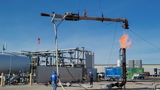
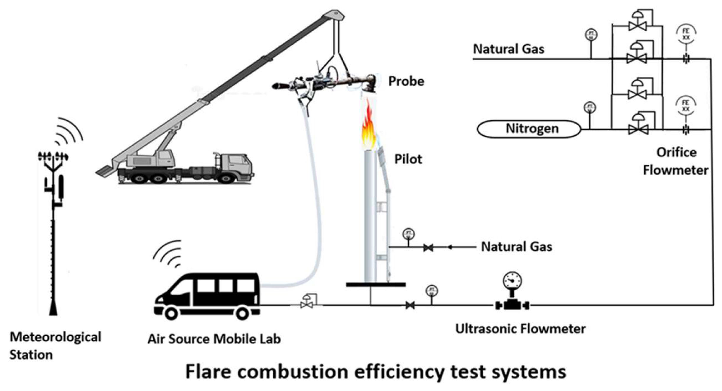
2.1. Experimental Apparatus

All measurements were conducted at the John Zink test facility in Tulsa, Oklahoma in January and February 2023. This facility has previously been used for related studies including the TCEQ flare study in 2010 [15] with updated mobile laboratory apparatus. There is currently no internationally recognized reference method for measuring flare combustion efficiency but it is considered by the authors to be the closest thing to a reference method currently available. The general layout of the experiment is shown in Figure 1.

Natural gas was supplied from Tulsa natural gas (TNG) from the gas grid with the addition of nitrogen to vary the net heating value of the gas mixture (NHV_vg) which is calculated as:

$${NHV}_{vg}={\sum }_{i=1}^n\left(\frac{{\%X}_{vg,i}}{100}\right){NHV}_i$$

(1)

where:

• NHV_vg = Flare vent gas net heating value, BTU/scf.
• i = Individual combustible component in flare vent gas.
• n = Number of individual combustible components in flare vent gas.
• %X_vg,i = Volume percentage of combustible component i in flare vent gas.
• NHV_i = Reported net heating value of combustible component i, BTU/scf.

The net heating value of vent gas (NHV_vg) is critical to whether a flare will light and keep burning. This is normally expressed for unassisted flares in BTU/scf with alternate equations also available for air- and steam-assisted flares to account for the role of these additional gases, such as NHV in the combustion zone (NHV_cz) and air dilution parameter (NHV_dil) [15]. In the United States, a minimum NHV_cz value of 270 BTU/scf is mandated for flares operated in refineries [24].

During the testing, TNG had a composition of C1 92.262%, C2 6.030%, C3 0.176%, CO₂ 0.497%, N₂ 1.025%. Nitrogen had a purity of 99.999%. A subset of tests added propylene to the gas mix to facilitate soot formation. The propylene supplied had a purity of >92%.

Gases were metered separately using orifice plate flowmeters with a ½” to 4” diameter orifice depending on flowrate and then mixed. All meters conform to ASME MFC-3M-2004 measurement standards [25]. In addition, the gas mixture was then measured using a 6-inch Panametrics ultrasonic flowmeter coupled with pressure and temperature probes and transmitters. The outputs from the flowmeter including flowrate and speed of sound were fed to the central data acquisition (DAQ) system.

Three custom-made flares were tested. The first (hereafter called the utility flare) was a 14-inch straight pipe flare with an effective diameter of 11 inches (95.03 in²). There is no restriction at the flare tip and it is representative of the simplest flare designs in operation. The second (hereafter called the sonic flare) is a single-arm 8-inch pressure-assisted flare in which the effective diameter at the tip is restricted by the inclusion of a metal cone creating an effective cross-sectional area of 21.7 in². The restricted tip creates an accelerated exit velocity intended to facilitate turbulent mixing with the air as an aid to combustion. The third tip (hereafter called the hydra) is a multi-arm design in which the input 8-inch flow of gas is split across seven restricted exits. The cumulative area of the orifices is 21.73 in² and is therefore close to that of the sonic tip. Testing of the sonic tip and hydra are used to evaluate the impact of changing flare design on combustion. It is acknowledged that the size of these flares is considerably smaller than many operational flares, some of which can exceed 100 inches in diameter, but is at the limits of what can be tested with the current technology.

The gas mixture was flowing in a 14-inch diameter pipe, reduced to 8 inches at the base of the flare for the sonic and hydra tests. The elbow in the flare pipe close to the ground may result in asymmetry in the flow through the flare tip. This was not investigated as part of this study.

The experimental design included the use of a single independent 2-inch flare pilot. The pilot was operated with a fixed independent fuel supply of TNG of the same origin and composition as used in the main flare. It had a constant flow of 87 scfh and was designed to operate with an effective CE/DRE of 100%. The experimental protocol includes consideration of the role of the pilot in deriving CE/DRE under a range of conditions.

The extraction device consists of an inlet cone, a sample preparation section, a sample extraction section, and eductor. The inlet face of the cone is 20” in diameter tapered to a 12” outlet. Around the perimeter of the cone, 120° apart, are three exposed junction thermocouples for sensing the temperature of the plume. The 12” cone outlet is connected to a 90-degree elbow in which mixing tabs have been installed. The mixing tabs ensure the plume sample that is pulled through the extraction apparatus is well mixed. The outlet of the elbow is connected to the inlet of the sample preparation section. The sample preparation section is a 9.5′-long 12” pipe with a Vortab flow conditioner located in the first 3 feet. The Vortab flow conditioner also assists in mixing the gases as well as conditioning the flow profile. At the exit of the sample preparation section is the extraction section. The sampling section is 1.5 feet long and consists of a pitot tube for measurement of the flue gas velocity in the apparatus, an exposed junction temperature element, and a flue gas extraction probe. The flare flue gas sample was obtained from this location. Downstream of the sampling section 7.5 feet is the end of the sample gas extraction apparatus where the eductor is attached. The eductor uses compressed air to induce flow through the apparatus. The sample gas extraction apparatus is designed with lifting lugs to allow it to be positioned with a crane; it is also designed with guide chains that will allow it to be positioned from the ground to prevent the apparatus from swinging and manual adjustment to allow precise positioning over the plume.

A representative exhaust sample of the flare emissions was collected through the sample gas extraction apparatus positioned over the exhaust plume of the flare. The sampling apparatus cone was positioned outside the visible flame and the position of the inlet adjusted so that the average temperature readings of the three inlet thermocouples are between 300° and 700 °F. The temperature of the gases entering the extraction was kept below 800 °F (the auto-ignition temperature of methane (1076 °F) and carbon monoxide (1128 °F) so that the combustion process has ceased prior to the sample being extracted. A heated sample line carries the sample into a mobile laboratory for analysis.

A weather station located in an open field about 400 feet away from the test spot measuring barometric pressure, ambient temperature, relative humidity and wind speed was connected to the DAQ system using wireless communication.

2.2. Analytical Protocol

All pre- and post-combustion analysis of gases were performed in near real-time using a mobile laboratory located on site. All laboratory equipment was operated and maintained as per manufacturer specifications.

Samples of the fuel gas flowing to the flare were collected from a point near the burner to confirm the composition and heating value of the fuel gas stream. A minimum of two samples during each test run were analyzed in accordance with EPA Method 18 [26] using a separate Fourier transform infra-red spectrometer (FTIR). The temperature and pressure of the fuel gas were measured at a location just upstream of the test burner. These measurements acted as a check to ensure that the flow rate through the metering system corresponds to these readings.

A portion of the sample combustion gas was analyzed on a wet basis (total hydrocarbons and GC analysis) to avoid condensation of the hydrocarbons prior to measurement. The remainder of the sample was dried and sent to the CO, O₂ and CO₂ analytical instruments.

The moisture content of the plume was calculated using a combination of Equations (13)–(19) and (19)–(34) of EPA Method 19 [27]. The total hydrocarbon concentration was then converted from a wet basis to a dry basis, and then the concentration on a dry basis was used in the remainder of the emission calculations.

Mass emission rates were determined by the stoichiometric calculation techniques of EPA Method 19 [27].

CO concentrations were determined in accordance with procedures set forth in EPA Method 10 using a continuous non-dispersive infrared (NDIR) analyzer (Thermo 48iHL) [28]. The NDIR analyzer was equipped with a gas correlation filter that removes any interference from CO₂ or other combustion products; this eliminates the need for ascarite traps. For values less than 1000 ppm, the meter is accurate to 0.1 ppm.

The CO₂ concentration measurements were made in accordance with the procedures of EPA Method 3A [29]. An infrared absorption CO₂ analyzer was utilized for these measurements (Servomex 1440). The instrument is accurate to 0.1% of reading.

The O₂ concentration measurements were made in accordance with the procedures of EPA Method 3A [29]. A paramagnetic cell O₂ analyzer was utilized for these measurements (Servomex 1440). The instrument is accurate to 0.1% of reading. The oxygen concentration is measured so that the amount of dilution air that has mixed with the sampled products of combustion can be determined.

EPA Method 25A was used to determine concentrations of total hydrocarbons [30]. Calibrated on a methane basis, the analyzer comprises a flame ionization detector to determine THC (Thermo 51i). For values less than 1000 ppm, the meter is accurate to 0.1 ppm.

The CE was calculated according to:

$$CE\%=\frac{\mathrm{10,000}\times X{CO}_2}{\left(\mathrm{10,000}\times X{CO}_2+XCO+XTHC\right)}\times 100$$

(2)

• where XCO₂, XCO and XTHC are dry gas concentrations of CO₂ in percentage, CO and total hydrocarbons in PPM as dry CH₄, respectively.

Dry gas concentrations of CO₂ and CO of the sampled flue gas were directly measured by the gas analyzers in the mobile lab. The total hydrocarbon concentration was measured on a wet basis and was converted to dry basis by accounting for total moisture content in the flue gas.

DRE was calculated according to:

$$DRE\%=\left(\frac{1-exTHC}{fTNG}\right)\times 100$$

(3)

where exTHC is the exhaust of total hydrocarbon in lbs/hr, and fTNG is the fuel mass flow rate of TNG in lbs/hr. The exhaust of total hydrocarbon, exTHC can be calculated based on the tracer gas of CO₂ or O₂ using standard US EPA method 19, 25A [30]. From the measured hydrocarbon concentration and the dilution ratio calculated from O₂ or CO₂ tracer gas, exTHC can be calculated.

Each test data point required 5 min of testing for a valid measurement and was repeated three times consecutively whilst monitoring the extraction thermocouples to ensure sampling remained within the plume. If the temperature dropped, the test period was extended. Raw data were inspected manually to ensure that measurements had fully accounted for the lag time between adjustment to the flow regime and the samples reaching the sampling analyzer.

At the scale of the test facility, the pilot gas (87 scfh TNG) flowrate is non-negligible compared to TNG gas in the flare flow and its effect on the measured CE/DRE needs to be accounted for. The pilot used is of standard design, which is not scaled for smaller flares such as those tested in these experiments. For correction on CE, it is assumed that the pilot gas burns at 100% CE and will release CO₂ into the plume of main flare. The pilot gas effect on CE can be corrected by accounting for CO₂ generated from the pilot gas. The CO₂ produced by pilot gas can be calculated based on the ratio between the TNG flowrate of vent gas and the TNG flowrate of the pilot. Assuming all the flue gases have the same dilution ratio, CO₂ produced by the pilot can be calculated as:

$${CO}_{2 pilot}={CO}_{2 dry}\times \frac{fTNGpt}{\left(fTNGvg+fTNGpt\right)}$$

(4)

where:

CO₂_pilot is CO₂ generated by pilot gas that could be detected by the analyzer.

CO₂_dry is the measured dry CO₂ concentration by the CO₂ analyzer.

fTNGpt is the pilot gas TNG flowrate (87 scfh).

fTNGvg is the TNG flowrate of the vent gas in scfh.

The effect of CO₂ produced by pilot gas is removed by:

$${CO}_{2 eff}={CO}_{2 dry}-{CO}_{2 pilot}={CO}_{2 dry}\times \frac{fTNGvg}{\left(fTNGvg+fTNGpt\right)}$$

(5)

where:

CO_2eff is the effective CO₂ produced by vent gas combustion.

Using the effective CO_2eff, CE is calculated with the correction of pilot gas effect.

The pilot effect on DRE calculation is mainly on oxygen depletion measurement. Oxygen depletion happened due to burning of fuels from both vent gas and pilot gas. It will affect the moisture calculation and hence the total hydrocarbon wet to dry gas concentration conversion. Oxygen depletion is also proportional to fuel flowrate. So, the pilot gas effect on oxygen depletion can be deduced from total oxygen depletion.

OD_total = 20.9 − O₂v%;

(6)

where:

OD_total is total oxygen depletion due to combustion of both vent gas and pilot gas.

O₂v% is the measured dry oxygen concentration in volume %.

Ambient air oxygen concentration is constant at 20.9%.

Oxygen depletion due to pilot gas can be calculated as:

OD_pilot= (20.9 − O₂v%) × fTNG_pt /(fTNG_vg + fTNG_pt)

(7)

and oxygen depletion due to vent gas can be calculated as:

OD_vg= (20.9 − O₂v%) × fTNG_vg/(fTNG_vg + fTNG_pt)

(8)

The effective oxygen dry volume percentage is:

O₂v%_eff = O₂v% − OD_vg

(9)

Using the effective O₂v%eff, DRE can be calculated with the correction of pilot gas effect.

2.3. Experimental Design

A test matrix was designed to test the three flare types under a range of flow rates and gas compositions, with particular focus on the conditions at which previous research has indicated that unstable combustion begins and where the need to assess CE/DRE is therefore most critical.

The net heating value of the gas was adjusted by blending Tulsa natural gas (TNG) with nitrogen. The composition and blended composition were periodically tested as described above. NHV_vg values range from 100% TNG giving 930 BTU/scf down to 17% TNG with a NHV_vg of 156 BTU/scf below which combustion could not be maintained.

As an open combustor, a flare is subject to enviromental conditions, specically crosswind. Wind can enhance flare combustion by creating turbulence and entraining air required for combustion. It could also strip the fuel out of the combustion zone before completion of the combustion, especially for high wind speeds [11]. Flare flowrate, which corresponds to exit velocity for a given flare tip with a known effective flare tip diameter, has a similar effect on flare performance as crosswinds. MFR or the ratio of exit velocity to wind speed are the parameters commonly used to descibe these two interrelated factors for flare combustion. MFR is defined as the ratio of the momentum flux of the gas jet at the flare tip to the momentum flux of the ambient air according to:

$$MFR=\frac{{\rho }_{vg}·{V_{vg}}^2}{{\rho }_{air}·{V_{wind}}^2}$$

(10)

where:

• MFR = Calculated momentum flux ratio, unitless.
• ρ_vg = Density of flare waste gas, lb/scf.
• V_vg = Flare vent gas velocity, ft/s.
• V_wind = Wind velocity, ft/s.
• r_air = Density of ambient air (constant of 0.07492), lb/scf.

Even though wind speed is uncontrolled, exit velocity can be controlled through flare flowrate to affect MFR or exit velocity over the crosswind ratio to replicate different flow regimes that may impact DRE.

The flow of gas was adjusted to yield exit velocities of 0.2 m/s, 0.6 m/s and 5 m/s. Under ambient weather conditions (<5 m/s crosswind), these were selected to yield a range of momentum flux ratio (MFR) conditions.

The design of test cases considers all the controllable parameters of flare operation: vent gas flowrate and heating value for each flare tip. At ambient crosswind conditions during the testing, MFR values ranged from 5 · 10⁻⁴ to 32, which covers the low MFR (<0.1) and wake-dominated flame (MFR > 3) regions. Vent gas containing a small portion of propylene gas was tested to gain insight to the effect of heavier hydrocarbons on natural gas combustion, especially at low NHV conditions.

3. Results

A complete set of experimental results are provided in the Supplementary Materials (https://zenodo.org/doi/10.5281/zenodo.10732509) accessed on 1 March 2024. In total, 87 experiments were successfully completed, comprising 26 utility flare, 41 sonic flare and 20 hydra flare tests. No test data have been excluded from the analysis, except where technical faults in the mobile laboratory and/or where the flare could not be kept lit for three replicate measurements of at least 5 min duration. Six measurements were conducted with the addition of propylene using sonic flare.

Uncertainty of the measurements was calculated in accordance with the Guide to Expression of Uncertainty in Measurement, often referred to as the GUM (ISO/IEC Guide 98-3:2008) [31] For CE/DRE measurement, uncertainty was introduced by instrument errors and sample extraction variations with the assumption of normal distribution for all the measurements. CE/DRE uncertainty was derived based on uncertainties of all the inputs (flue gas concentration measurement, such as CO₂, CO and total hydrocarbon content (THC), flare gas composition measurement) and their sensitivity coefficients. The uncertainty caused by gas sampling can be estimated from the standard deviation of the replicate CE/DRE measurement. The overall uncertainty is calculated as the root sum square of the instrument error and sample extraction error. As such, each result is expressed with its own unique uncertainty value rather than applying a single value to all tests. This helps to identify how uncertainty changes along with the CE/DRE and its implications for emissions reporting.

The results submitted include the measured CE and DRE values and the CE and DRE values once corrected for the impact of the pilot. The average of the three corrected measurements is presented along with an estimate of the uncertainty.

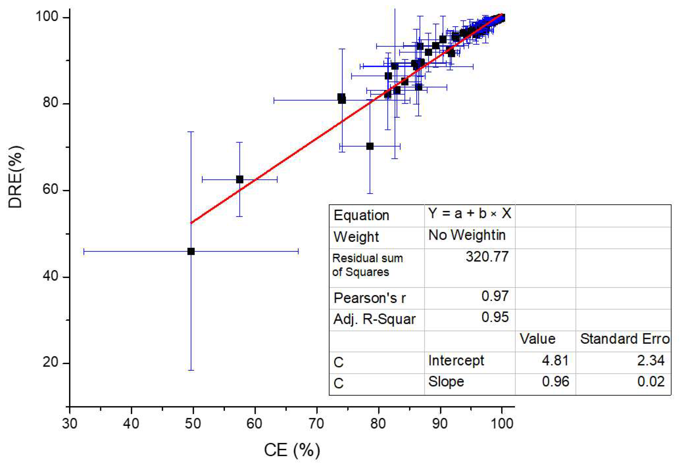
3.1. Relationship between CE and DRE Values

Efficiency of flare combustion can be measured by combustion efficiency (CE) or destruction and removal efficiency (DRE). While CE measures the flare gas that undergoes complete combustion converting into CO₂, DRE measures flare gas converting into complete and incomplete combustion products. DRE would have a higher value than CE for a given measurement with the difference decreasing with increasing CE because of a less incomplete combustion product at a higher combustion efficiency. There is a strong correlation between CE and DRE as shown in Figure 2. A linear fit of DRE versus CE yields a slope of 0.9604 and an offset of 4.81% for all the data points measured in this test. Under the majority of test cases, the DRE exceeds 98% with CE and DRE being indistinguishable close to complete combustion at the level of uncertainty achievable under experimental conditions. This linear relationship between CE and DRE explains why they are often interchangeable in flare efficiency measurement. Since methane emission from flaring is calculated from DRE and flowrate as shown in Equation (3), subsequent analysis will be focusing on DRE from a methane emission perspective.

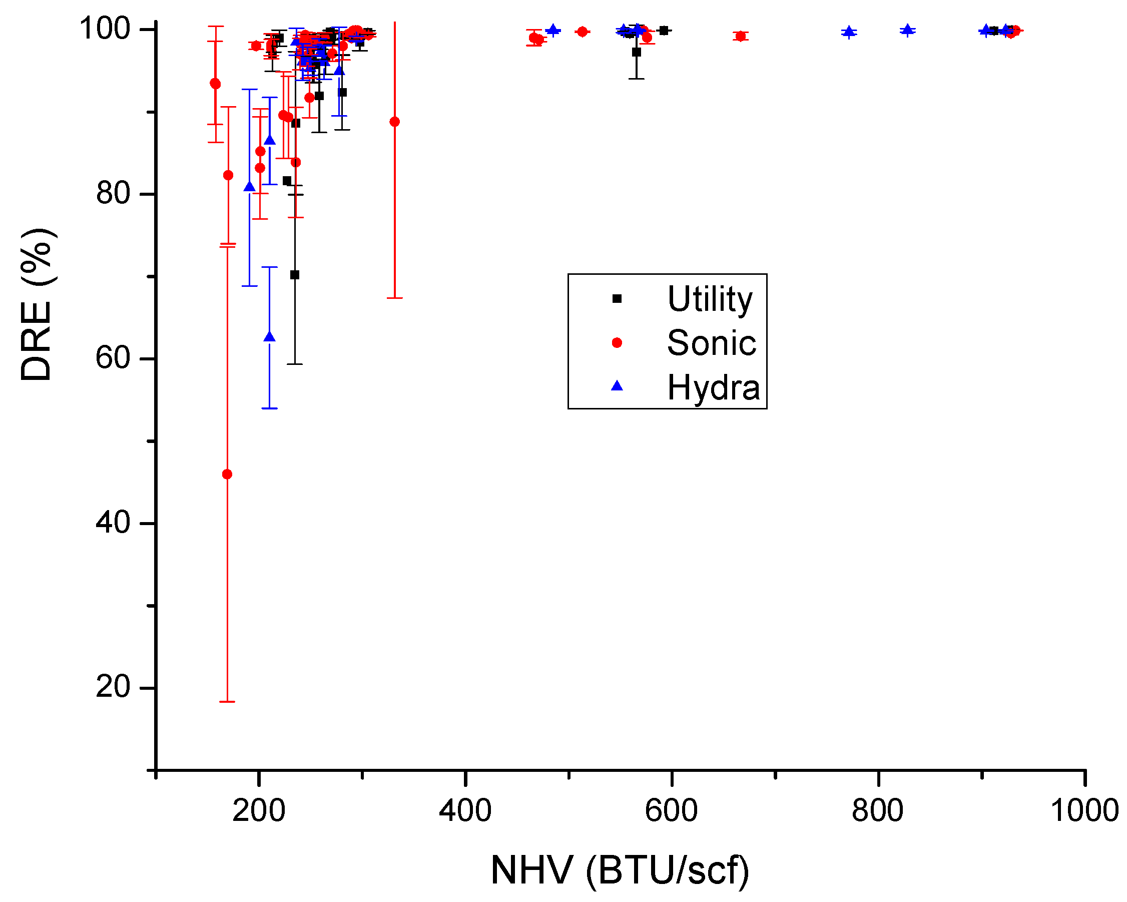
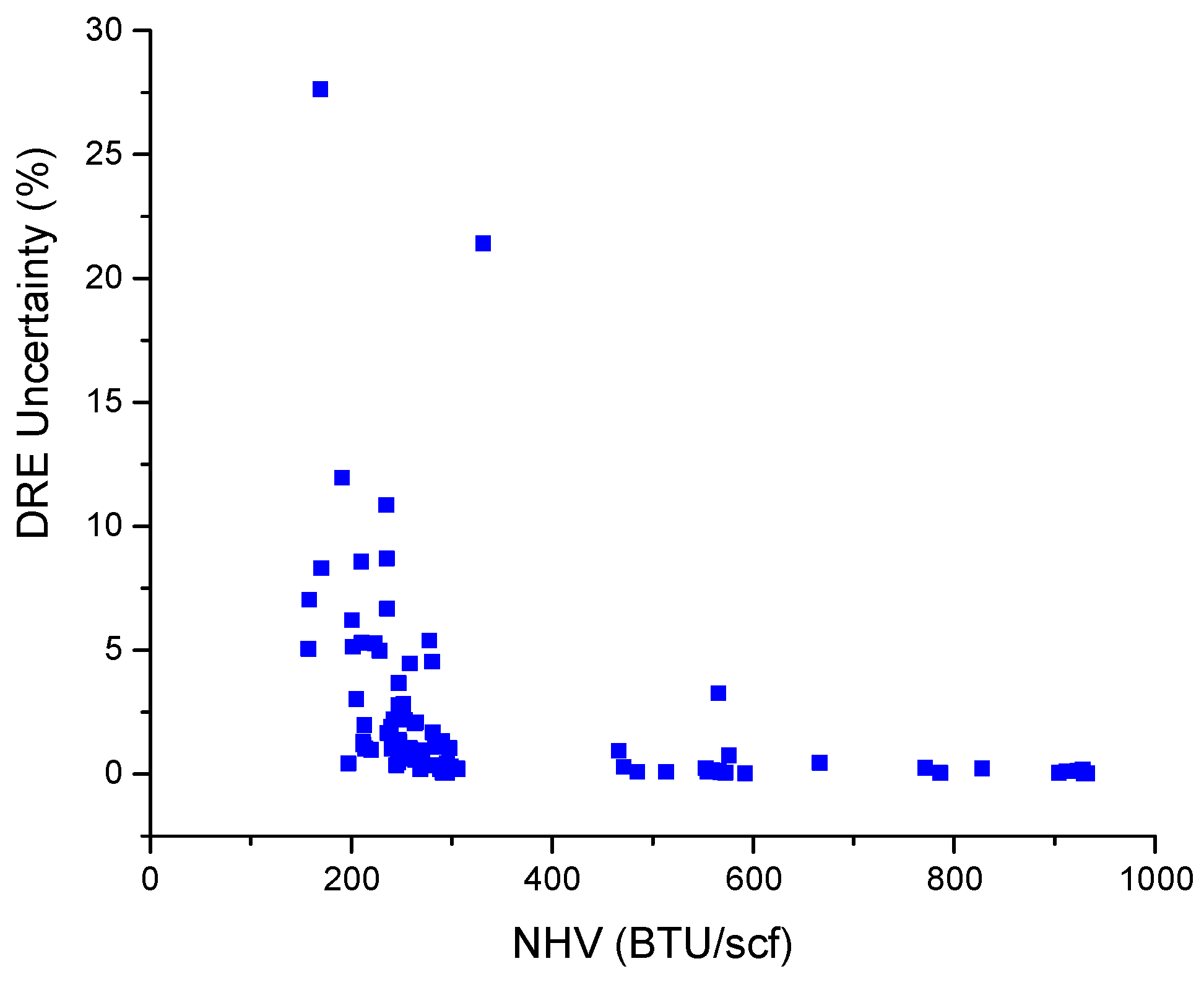
3.2. Impact of Net Heating Value on DRE

One of the key parameters affecting flare efficiency is flare gas heating content. Shown in Figure 3 is the measured DRE vs NHV for all the test points with its corresponding uncertainty. The DRE measured for all the test points showed a very high value for the NHV > 300 BTU/scf region with an average value of 99.69%, with very little variations caused by flowrate or wind speed under all the conditions during the test. DRE showed a rapid transition for NHV from 200 BTU/scf to 300 BTU/scf with DRE varying from 46% to >98%. The measurement uncertainty in this region also showed a similar trend as the DRE value itself.

The measured DRE for three different flare tips was plotted using different colors and shapes in Figure 3. For all the flowrates tested with the exit velocity ranging from 0.2 m/s to 5 m/s and ambient wind speed up to 14 mph, no noticeable difference between the three tip designs was observed, beside the fact that flare gas NHV is one of the dominating factors affecting flare DRE and DRE showed a similar trend for all three tips.

The DRE results with propylene in the NHV region from 200 BTU/scf to 300 BTU/scf showed a slightly higher value than the TNG counterpart. For example, the testing conditions for experiments PP2 and GB17AR1 are almost identical in terms of flowrate, heating value and wind speed, while the DRE measured for propylene is much higher, 90.18% comparing to 86.95%. The relatively high DRE is most likely resulted from the higher flammability of propylene gas.

Figure 4 shows the change in measurement uncertainty as a function of net heating value. Above 300 BTU/scf (where combustion is >98% DRE), the uncertainty of individual experiments have a median average of ±0.11 (1 σ), including outliers with values up to 0.46%. Below 300 BTU/scf, there is a rapid deterioration in the uncertainty of individual measurements.

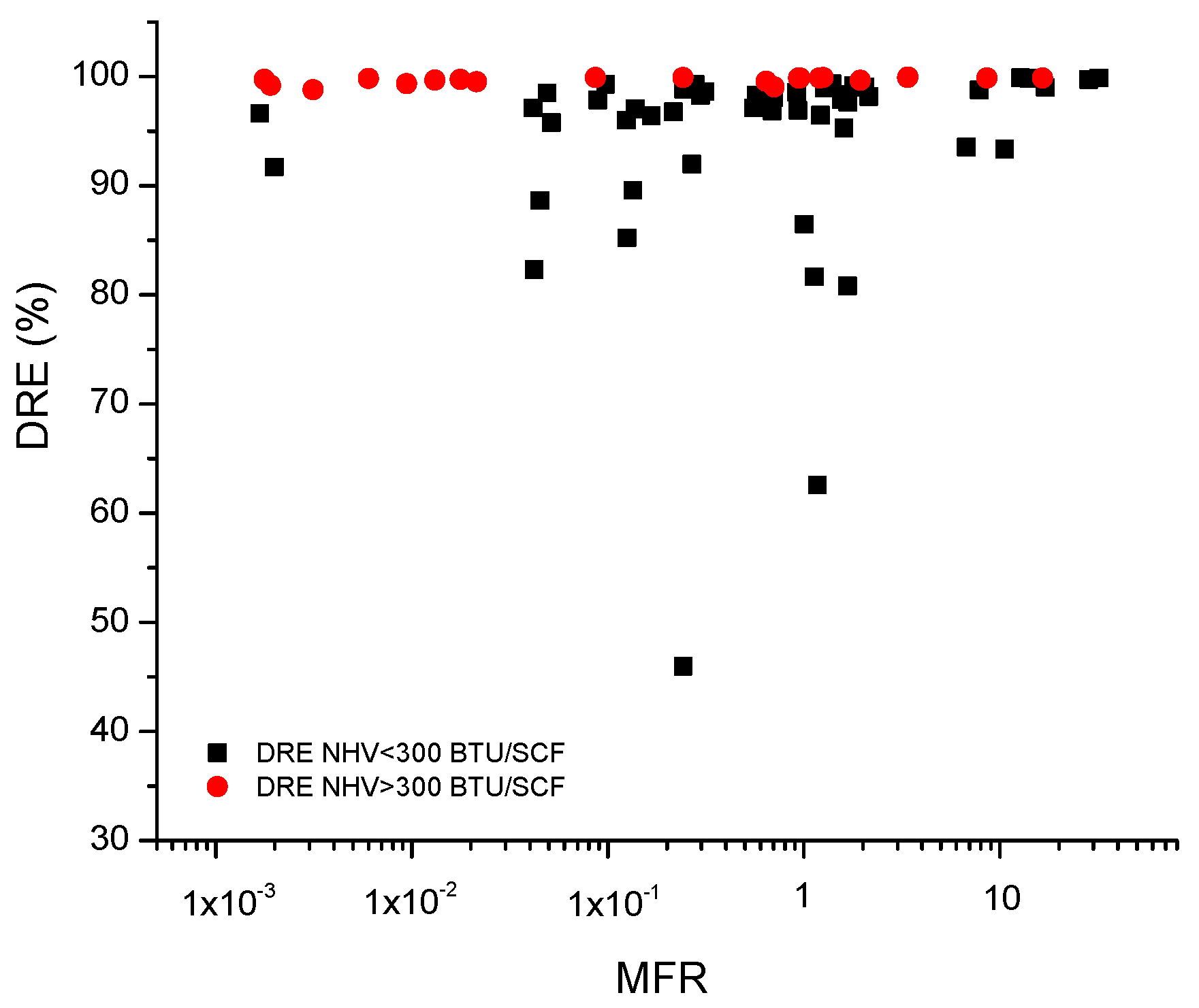
3.3. Influence of Flow and Crosswind on DRE

The test cases in this paper cover a wide range of MFR, from 0.0005 to 32. Under experimental conditions, this variation is primarily a function of gas flow rate as ambient wind speeds did not exceed 15 mph. Plotted in Figure 5 is the measured DRE against MFR. Under these benign conditions, MFR has a secondary influence on DRE. As shown in the plot, for the NHV > 300 BTU/SCF region, DRE is maintained at very high values (>99%) with a minimum effect from MFR. For NHV < 300 BTU/SCF, there is a pronounced DRE with MFR < 1.

4. Discussion

Determining the destruction efficiency of individual flares is essential if the impact of flaring on methane emissions is to be fully evaluated and mitigated. For flares without steam or air assistance, DRE values of >98% can be maintained providing the NHV_vg of the gas is known and maintained at >300 BTU/scf and the flare is kept lit. Assessing the risk to a flare of high crosswind conditions requires more than can be achieved in full-scale empirical testing.

Many current reporting requirements assume 98% DRE under all flow, composition and weather conditions. This needs to be revised to better reflect the conditions that drive flares into lower DRE. Measurement of the performance of individual flares under their specific range of operational conditions is needed to identify those flares where conditions are sub-optimal. Moreover, continuing to report all flares as 98% efficient may result in an over-estimation of the contribution of flaring to methane inventories and divert resources away from other mitigation efforts.

The uncertainty of the measurements may appear small (typically an absolute uncertainty of 0.5% in high DRE cases) but when applied to operational flares a difference of 0.5% can equate to material differences in emissions. A shift in reported emissions from a flare of 98 to 98.5% drops the methane emissions by 25%. Where flares dominate the methane inventory, such as in many offshore locations, a 25% shift in flaring is more material than other sources such as fugitives. However, such a shift can only be considered a defensible emission reduction if the change is greater than the uncertainty of the measurement. To make this possible, a step change is required in the assessment of flare performance. This shall require a new generation of measurement standards that can evaluate flare performance under a wide range of operational conditions. This is a significant challenge; in-field empirical studies will be limited by the operational difficulties of extractive sampling and the inability to control the weather. Scaled experiments, such as the use of wind tunnels, may be challenged by their capacity to replicate the complex designs found in many large flares including those with multi-arm geometries or where the tip geometry can dynamically change with flow. Computational methods such as fluid dynamics may offer a pragmatic solution, but there are currently no standards or guidelines as to how these are best validated and applied to flares.

Under operational conditions, a flare may be subject to a wide range of flow, composition and wind speeds. Where there is a risk that low DRE conditions can be encountered, it is important that continuous tracking of the flare DRE is conducted. This is underpinned by the need for accurate metering (which is not universal on all flares) and a means by which changes in composition can be tracked. The periodic assessment of flares may struggle to take measurements during safety flaring events or during high winds.

Many flares around the world are not equipped with the means to fully measure flow and composition on an ongoing basis, especially smaller flares found in the onshore market and in developing countries. However, even offline assessments of the NHV_vg of the gas and precautions taken to maintain an effective pilot can make a material, if hard to measure, contribution to lowering methane emissions.

5. Conclusions

Measuring and then reducing methane from flaring represent a significant part of how the oil and gas industry can reduce their contribution to global methane emissions. Alongside the challenge of unlit flares, ensuring that the efficiency is kept high is important as small shifts in DRE can equate to significant changes in the total methane emitted. However, this can be difficult to assess as the flare may be subject to variations in flow and gas composition and subject to the effect of crosswinds.

Empirical testing of flares has demonstrated that the universal application of 98% DRE to methane reporting needs to be revised and highlighted the importance of tracking flare performance if the role of flares as a source of methane to the atmosphere is to be reported and is the basis for tangible, defensible and sustainable emissions reductions.

These results can help inform and evaluate a new generation of models used to provide improved information on flare performance and how changes in flow, composition and environmental conditions can all affect that value. Even where the application of such systems may not be currently feasible, such as where metering is limited or where compositional analysis is periodic, the data may be used to help assess whether an installed flare is likely to be at risk of delivering lower DRE values. Where more detailed data are available, it can form the basis of calculating a site-specific DRE figure.

The uncertainty of the measurements, with an absolute value of 0.5%, can equate to potentially substantial differences in the amount of methane thought to be emitted. Further improvements in the accuracy with which methane from flaring can be reported therefore requires a new generation of reference methods.

References

1. Myhre, G.; Shindell, D.; Bréon, F.-M.; Collins, W.; Fuglestvedt, J.; Huang, J.; Koch, D.; Lamarque, J.-F.; Lee, D.; Mendoza, B.; et al. Anthropogenic and Natural Radiative Forcing. In Climate Change 2013: The Physical Science Basis. Contribution of Working Group I to the Fifth Assessment Report of the Intergovernmental Panel on Climate Change; Stocker, T.F., Qin, D., Plattner, G.-K., Tignor, M., Allen, S.K., Boschung, J., Nauels, A., Xia, Y., Bex, V., Midgley, P.M., Eds.; Cambridge University Press: Cambridge, UK; New York, NY, USA, 2013. [Google Scholar]
2. Etminan, M.; Myhre, G.; Highwood, E.J.; Shine, K.P. Radiative forcing of carbon dioxide, methane, and nitrous oxide: A significant revision of the methane radiative forcing. Geophys. Res. Lett. 2016, 43, 612–614. [Google Scholar] [CrossRef]
3. Ocko, I.B.; Sun, T.; Shindell, D.; Oppenheimer, M.; Hristov, A.N.; Pacala, S.W.; Mauzerall, D.L.; Xu, Y.; Hamburg, S.P. Acting rapidly to deploy readily available methane mitigation measures by sector can immediately slow global warming. Environ. Res. Lett. 2021, 16, 054042. [Google Scholar] [CrossRef]
4. Jackson, R.B.; Saunois, M.; Bousquet, P.; Canadell, J.G.; Poulter, B.; Stavert, A.R.; Bergamaschi, P.; Niwa, Y.; Segers, A.; Tsuruta, A. Increasing anthropogenic methane emissions arise equally from agricultural and fossil fuel sources. Environ. Res. Lett. 2020, 15, 071002. [Google Scholar] [CrossRef]
5. Global Methane Pledge. Available online: https://www.globalmethanepledge.org (accessed on 1 November 2023).
6. Bamji, Z. Global Gas Flaring Tracker Report, March 2023; World Bank Publications: Washington, DC, USA, 2023. [Google Scholar]
7. Corbin, D.; Johnson, M. Detailed Expressions and Methodologies for Measuring Flare Combustion Efficiency, Species Emission Rates, and Associated Uncertainties. Ind. Eng. Chem. Res. 2014, 53, 19359–19369. [Google Scholar] [CrossRef]
8. Parameters for Properly Designed and Operated Flares. Report for Flare Review Panel, April 2012 U.S. EPA Office for Air Quality Planning and Standards (OAQPS). Available online: https://www3.epa.gov/airtoxics/flare/2012flaretechreport.pdf (accessed on 6 October 2023).
9. Freeke, J.; Chong, T.; Newman, D.; Evans, P. Realtime methane quantification and reporting with upstream flaring. In Proceedings of the Global Flow Measurement Workshop, Tonsberg, Norway, 24–27 October 2023. [Google Scholar]
10. Johnson, M.R.; Kostiuk, L.W. Efficiencies of low-momentum jet diffusion flames in crosswinds. Combust. Flame 2000, 123, 189–200. [Google Scholar] [CrossRef]
11. Johnson, M.R.; Wilson, D.J.; Kostiuk, L.W. A Fuel Stripping Mechanism for Low-momentum Jet Diffusion Flames in a Crossflow. Combust. Sci. Technol. 2000, 169, 155–174. [Google Scholar] [CrossRef]
12. EEMS Atmospheric Emission Calculations Issue 1.8; UK Offshore Operators Association Ltd.: Aberdeen, UK, 2008.
13. McDaniel, M. Flare Efficiency Study; Environmental Protection Agency: Washington, DC, USA, 1983; EPA-600/2-83-052.
14. Pohl, J.; Soelberg, N. Evaluation of the Efficiency of Industrial Flares: Flare Head Design and Gas Composition; EPA: Washington, DC, USA, 1985. Available online: https://nepis.epa.gov/Exe/ZyPDF.cgi/P1003QL1.PDF?Dockey=P1003QL1.PDF (accessed on 6 October 2023).
15. Allen, D.; Torres, V. Flare Study Final Report. Texas Commission on Environmental Quality PGA No. 582-8-862-45-FY09-04Tracking No. 2008-81 with Supplemental Support from the Air Quality Research Program TCEQ Grant No. 582-10-94300 TCEQ 2010 Flare Study Final Report. Available online: http://www.d7036.com/home/downloads_server/2010-flare-study-final-report.pdf (accessed on 1 October 2023).
16. Plant, G.; Kort, E.A.; Brandt, A.R.; Chen, Y.; Fordice, G.; Gorchov Negron, A.M.; Schwietzke, S.; Smith, M.; Zavala-Araiza, D. Inefficient and unlit natural gas flares both emit large quantities of methane. Science 2022, 377, 1566–1571. [Google Scholar] [CrossRef] [PubMed]
17. Shaw, J.T.; Foulds, A.; Wilde, S.; Barker, P.; Squires, F.A.; Lee, J.; Purvis, R.; Burton, R.; Colfescu, I.; Mobbs, S.; et al. Flaring efficiencies and NOx emission ratios measured for offshore oil and gas facilities in the North Sea. Atmos. Chem. Phys. 2023, 23, 1491–1509. [Google Scholar] [CrossRef]
18. OGMP Technical Guidance Document—Flare Efficiency. Available online: https://ogmpartnership.com/wp-content/uploads/2023/02/Flare-efficiency-TGD-Approved-by-SG.pdf (accessed on 6 October 2023).
19. Few, J. Review of Differential Absorption Lidar Flare Emission and Performance Data; Chief Scientist’s Group report October 2019 Version: SC150026/R (HOEV151612 Task 1); Environment Agency: London, UK, 20 October 2019; ISBN 978-1-84911-434-9.
20. Black, S. Metering and Emission Analysis of Flare and Vent Metering Systems Using Computational Fluid Dynamics. In Proceedings of the Global Flow Measurement Workshop, Aberdeen, UK, 20–21 October 2022. [Google Scholar]
21. Zeng, Y.; Morris, J.; Dombrowski, M. Validation of a new method for measuring and continuously monitoring the efficiency of industrial flares. J. Air Waste Manag. Assoc. 2016, 66, 76–86. [Google Scholar] [CrossRef] [PubMed]
22. Tao, C.; Chow, J.; Sui, L.; Wang, A.; Freeke, J.; Zhang, J.; Evans, P.; Newman, D.; Venuturumilli, R.; Lowe, J.; et al. Validation of a new method for continuous flare combustion efficiency monitoring. Atmosphere 2024. [Google Scholar]
23. Peebles, B.; Stockton, P. Offshore flares: Measurement and calculation of combustion efficiency, methane and CO2e emissions. In Proceedings of the North Sea Flow Measurement Workshop, Aberdeen, UK, 20–21 October 2022; Available online: https://s3.eu-west-2.amazonaws.com/assets.accord-esl.com/2022-Offshore-Flares-Measurement-and-Calculation-of-Combustion-Efficiency-Methane-C02e-Emissions_NSFMW-2022_Accord-ESL.pdf (accessed on 6 October 2023).
24. US EPA, 40 CFR Parts 60 and 63. Available online: https://www.govinfo.gov/content/pkg/FR-2018-11-26/pdf/2018-25080.pdf (accessed on 1 November 2023).
25. ASME Standard MFC-3M-2004; Measurement of Fluid Flow in Pipes Using Orifice, Nozzle, and Venturi. ASME: New York, NY, USA, 2004.
26. EPA Method 18—Measurement of Gaseous Organic Compound Emissions by Gas Chromatography. Available online: https://www.epa.gov/emc/method-18-volatile-organic-compounds-gas-chromatography (accessed on 13 November 2023).
27. EPA Method 19—Determination of Sulfur Dioxide Removal Efficiency and Particulate Matter, Sulfur Dioxide, and Nitrogen Oxide Emission Rates. Available online: https://www.epa.gov/emc/method-19-sulfur-dioxide-removal-and-particulate-sulfur-dioxide-and-nitrogen-oxides-electric (accessed on 13 November 2023).
28. EPA Method 10—Determination of Carbon Monoxide Emissions from Stationary Sources (Instrumental Analyzer Procedure). Available online: https://www.epa.gov/emc/method-10-carbon-monoxide-instrumental-analyzer (accessed on 13 November 2023).
29. EPA Method 3A—Oxygen and Carbon Dioxide Concentrations–Instrumental. Available online: https://www.epa.gov/emc/method-3a-oxygen-and-carbon-dioxide-concentrations-instrumental (accessed on 13 November 2023).
30. EPA Method 25A—Determination of Total Gaseous Organic Concentration Using a Flame Ionization Analyzer. Available online: https://www.epa.gov/emc/method-25a-gaseous-organic-concentration-flame-ionization (accessed on 13 November 2023).
31. ISO/IEC Guide 98-3:2008; Uncertainty of Measurement—Part 3: Guide to the Expression of Uncertainty in Measurement (GUM:1995). ISO: Geneva, Switzerland, 2008.
Figure 1. General configuration of extractive sampling experimental design.
Atmosphere 15 00333 g001
Figure 2. The relationship between CE and DRE with corresponding measurement errors for three designs under test. The insert table shows the linear fit results.
Atmosphere 15 00333 g002
Figure 3. Overall view of DRE vs NHV with corresponding error bar (1 s) for each point. DRE values for each flare design are color coded: back square is for utility flare, red circle is for sonic flare and blue triangle is for hydra flare.
Atmosphere 15 00333 g003
Figure 4. Change in measurement uncertainty (1 σ) as a function of net heating value.
Atmosphere 15 00333 g004
Figure 5. The relationship between MFR and DRE. Under test conditions, where NHV is >300 BTU/scf, a DRE of close to 100% is maintained. Low NHV gas (<300 BTU/scf) is more susceptible to low levels of combustion.
Atmosphere 15 00333 g005
Disclaimer/Publisher’s Note: The statements, opinions and data contained in all publications are solely those of the individual author(s) and contributor(s) and not of MDPI and/or the editor(s). MDPI and/or the editor(s) disclaim responsibility for any injury to people or property resulting from any ideas, methods, instructions or products referred to in the content.