Abstract
The monitoring of anthropogenic CO2 emissions, which increase the atmospheric CO2 concentration, plays the most important role in the management of emission reduction and control. With the massive increase in satellite-based observation data related to carbon emissions, a data-driven machine learning method has great prospects for predicting anthropogenic CO2 emissions. Training samples, which are used to model predictions of anthropogenic CO2 emissions through machine learning algorithms, play a key role in obtaining accurate predictions for the spatial heterogeneity of anthropogenic CO2 emissions. We propose an approach for predicting anthropogenic CO2 emissions using the training datasets derived from the clustering of the atmospheric CO2 concentration and the segmentation of emissions to resolve the issue of the spatial heterogeneity of anthropogenic CO2 emissions in machine learning modeling. We assessed machine learning algorithms based on decision trees and gradient boosting (GBDT), including LightGBM, XGBoost, and CatBoost. We used multiple parameters related to anthropogenic CO2-emitting activities as predictor variables and emission inventory data from 2019 to 2021, and we compared and verified the accuracy and effectiveness of different prediction models based on the different sampling methods of training datasets combined with machine learning algorithms. As a result, the anthropogenic CO2 emissions predicted by CatBoost modeling from the training dataset derived from the clustering analysis and segmentation method demonstrated optimal prediction accuracy and performance for revealing anthropogenic CO2 emissions. Based on a machine learning algorithm using observation data, this approach for predicting anthropogenic CO2 emissions could help us quickly obtain up-to-date information on anthropogenic CO2 emissions as one of the emission monitoring tools.
1. Introduction
Anthropogenic carbon dioxide (CO2) emissions, which account for 70% of the total greenhouse gas emissions [1], are the main contributors to the increasing atmospheric CO2 concentration. The continuous rise in the atmospheric CO2 concentration is causing global warming and the frequent occurrence of climate extremes [2], which are seriously impacting human life [3,4]. Consequently, controlling and reducing anthropogenic CO2 emissions has become the primary responsibility of every country in order to mitigate global warming [5]. The reduction in and control of anthropogenic CO2 emissions needs to be supported by keeping track of anthropogenic CO2 emissions. However, it is a challenge to predict anthropogenic CO2 emissions quickly and accurately [6].
The data on anthropogenic CO2 emissions are currently obtained using a bottom-up methodology [7]. Firstly, the total emissions are collected by countries and regional inventory statistics; then, they are redistributed to map the emissions at spatial and temporal scales using proxies such as population and nighttime lighting [8]. This methodology is based on the disaggregated accounting of national or regional energy-consuming sectors or industry sectors, which strongly depend on the standards, accuracy, and lag of the statistical methods in each country [9,10]. Moreover, the proxy data, which are used to map the emissions in space and time, have some uncertainty that affects the reliability of the regional emissions [11,12]. These emission statistics, proxies, and methodologies for the allocation of emissions introduce diverse uncertainties into the emission inventory [13,14].
A top-down data-driven approach for predicting anthropogenic CO2 emissions is currently being developed using massive data from multiple source measures, such as satellite remote sensing technology and the increase in available satellite-based parameter data [15,16]. The data-driven approach, which uses objective and current satellite observation data, can be a means to supplement the monitoring of anthropogenic CO2 emissions and to cross-reference the bottom-up emission inventory data [17]. The prediction models of anthropogenic CO2 emissions have been progressively developed from simple mathematical statistical models to complicated models based on machine learning algorithms with the advancement of big data technology [6,18,19]. Machine learning algorithms can model the relationships between emissions and relevant parameters impacting emissions by training and learning the relationships using massive data. With the increase and diversification of data related to carbon emissions, machine learning-based prediction methods for anthropogenic CO2 emissions have been under development as monitoring tools for anthropogenic CO2 emissions [20]. Several studies have proposed applying machine learning and deep learning models to estimate anthropogenic CO2 emissions, such as artificial neural networks (ANNs), generalized regression neural networks (GRNNs), random forests (RFs), radial basis functions (RBFs), and long short-term memory (LSTM) networks. The results have shown that these models demonstrated some prediction performances and potential for estimating anthropogenic CO2 emissions [21,22,23,24,25,26].
Anthropogenic CO2 emissions are primarily from industrial processes that involve the combustion of fossil fuels, which are closely linked to human activities [1,2]. These activities are mainly concentrated in urban centers and their surrounding regions, which result in a high geospatial aggregation of anthropogenic CO2 emissions. Consequently, the values of emissions have a regional non-normal distribution, which affects the unbiased modeling and accurate estimation of ACEs. Several studies have attempted to reduce this effect using the sampling methods of training data (e.g., by segmenting the emission intensity into two parts and then constructing an estimation model on a segment basis [27,28]) and demonstrated better validation results for predicting anthropogenic CO2 emissions at the national scale. However, these previous studies used few predictor variables and insufficiently evaluated the prediction results. They mostly focused on cross-validation and lacked an evaluation of how the model’s effectiveness was affected by the training data and available machine learning algorithms.
China is a country with some of the highest CO2 emissions and rapid economic development. The anthropogenic CO2 emissions in China are significantly concentrated in the eastern region, where there are highly dense populations and cities, industrial enterprises, and advanced economies. Meanwhile, fewer CO2 emissions originate in the western region with low-density populations, many rural areas, and fewer industrial enterprises due to harsh environments. Therefore, the anthropogenic CO2 emissions present in China are highly spatially inhomogeneous, as described above. As a major emitter, the control of and reduction in CO2 emissions in China will have a significant effect on mitigating global climate warming. The Chinese government is currently taking steps to reduce CO2 emissions and, thus, urgently needs accurate CO2 emission data. In this study, we took mainland China as the study area to develop an approach for accurately predicting CO2 emissions.
The aim of this study was to develop an optimal prediction model for anthropogenic CO2 emissions by optimizing training datasets from various sampling methods and available machine learning algorithms to address the problem of the non-normal distribution of emissions. We compared and verified the prediction results from different sampling and machine algorithm models to evaluate the effectiveness of modeling the relationships between anthropogenic CO2 emissions and the prediction parameters for the accurate prediction of anthropogenic CO2 emissions. The research in this paper will assist the government in accurately obtaining anthropogenic emission data and supporting the implementation of measures to reduce and control the anthropogenic emissions of CO2 by tracking them, thereby mitigating the impacts of global warming and safeguarding against climate change [29].
2. Materials and Methods
2.1. Data Acquisition and Preprocessing
Taking mainland China as the study area, we collected anthropogenic CO2 emission inventory data (ODIAC) from 2019 to 2021 and relevant parameters as predictive variables, including atmospheric CO2 concentration data (CO2), atmospheric NO2 concentration data (NO2), impervious surface cover (IS), nighttime lighting (NL), vegetation index (NDVI), and vegetation CO2 ecological uptake parameter data (SIF) related to anthropogenic CO2 emission activities. In addition, we used meteorological reanalysis data (ERA5): wind field data (10 m east–west wind speed (U10), 10 m north–south wind speed (V10)), 2 m temperature (T2M), and dew point temperature (D2M). The characteristics of each parameter and its data source are given in Table 1.

Table 1.
The collected parameters for predicting ACEs based on ML.
We collected ACE data from the Open-source Data Inventory for Anthropogenic CO2 (ODIAC). The ODIAC data were generated, and the national total emissions were reallocated on a spatial grid based on CARMA power plant data (power and geographic location) and DMSP/NPP nighttime lighting data [30]. These data are released as monthly averages with a resolution of 1 km × 1 km and cover the global continent. This is one of the most widely used carbon emission datasets [31].
The changes in atmospheric CO2 concentrations correspond significantly to ACE levels [32,33]. We collected monthly XCO2 data in a 0.1° × 0.1° grid from 2019 to 2021 and the monthly XCO2 dataset in a 1° grid from 2010 to 2021. These data are spatiotemporally continuous XCO2 data generated by spatiotemporal statistics and machine learning methods using the XCO2 retrievals from satellite observations, including GOSAT, OCO-2, and OCO-3 [18]. Atmospheric NO2 also mainly comes from the anthropogenic emissions of fossil fuel combustion, in which the CO2 emissions are usually accompanied by NO2 emissions [34]. The short-lived NO2 is more sensitive to changes in anthropogenic CO2 emissions compared to the short-lived CO2 [35]. Therefore, we collected the global monthly mean concentration data with a resolution of 0.01° from atmospheric NO2 data inverted from observations of the Tropospheric Monitoring Instrument (TROPOMI) on board the Sentinel-5P satellite [36]. The satellite-observed vegetation parameters SIF, NDVI, and meteorological reanalysis data (ERA5) are used to represent the effects of terrestrial ecology and atmospheric transport, as changes in atmospheric CO2 concentrations not only correspond to anthropogenic CO2 emissions but also depend on the CO2 release and uptake of terrestrial ecology and atmospheric transport [37,38]. Moreover, it was found that alterations to and destruction of vegetation ecology could intensify greenhouse gas emissions, which are the cause of climate warming [39].
Associated with human activities, the NL data are derived from the observations of the Suomi NPP satellite [40]. The IS is largely contributed by cities, which have strong impacts on anthropogenic CO2 emissions due to their economic development, energy consumption, industrial activities, and population concentration [41]. The IS can explain the spatial extent of human emission activities and make up for the impact of gaps in the nighttime lighting data. This study used the global 30 m impervious surface data produced by Zhang et al., which has higher overall precision and better accuracy than other data products [42]. The RN data demonstrate the impact of transportation factors on anthropogenic CO2 emissions.
The collected data shown in Table 1 are inconsistent in space and time. To address this, these data were processed to integrate them into a monthly mean in a 0.1° × 0.1° grid for predicting anthropogenic CO2 emissions in a 0.1° grid. The NL, NO2, ERA5, NDVI, and SIF data were sampled to a 0.1° grid by calculating the mean of the data located within a 0.1° grid. The ODIAC data were processed to a 0.1° grid using cumulative computing. To remove the effect of the background concentration of atmospheric CO2, thereby enhancing the CO2 signal from the local anthropogenic emissions, the difference (dXCO2) between the CO2 concentration and the background XCO2 was calculated for each grid, where the background XCO2 had the median value of the CO2 data from the same month in the study area [32]. The IS and RN data were sampled on a 0.1° × 0.1° grid by calculating the density of the data area within a 0.1° × 0.1° grid.
2.2. Methodology
Modeling anthropogenic CO2 emissions (hereafter, referred to as ACEs) based on machine learning (hereafter, referred to as ML) can be expressed by Equation (1):
where Y is the predicted ACE, Xn is the nth predictor variable related to ACEs and the atmospheric CO2 concentration, which are the parameters obtained from the satellite-based observations, and f is the predicting model function, which is derived from machine learning, which models the relationship between Y (based on ODIAC data here) and the prediction parameters (X1, X2, X3, ……, Xn), which are XCO2, NO2, NL, IS, SIF, NDVI, D2M, T2M, U10, V10, and RN, as shown in Table 1. A flowchart of the used data and prediction approach is given in Figure 1.
Y = f (X1, X2, X3, ……, Xn),
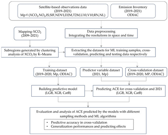
Figure 1.
Flowchart of the prediction approach and the used data.
2.2.1. Creation of Sample Datasets
In the first step, we needed to generate three datasets, including a training dataset, a cross-validation dataset, and a predictor variable dataset, for the entire studied area, as shown in Figure 1. These were used to derive the ACE prediction models, validate the models, and evaluate the performance of the predicted ACEs, respectively. The key processing methods included two steps in the framework of the approach, as shown in Figure 1. The first step was to generate efficient training datasets, which were used for the training and learning of the prediction model. The second was to evaluate the performances of the models predicting the ACE not only through cross-validation of the models but also through bias assessment of the predicted ACEs. Extracting data samples to generate the training datasets is essential to building an accurate ACE prediction model. To address the problem of the non-normal distribution of ACEs in the study area, we adopted the approach of extracting the training learning samples from the subregions of the study area to generate the training dataset for each subregion.
The subregions were obtained through clustering analysis of the spatiotemporal characteristics of the XCO2 data. It is known that XCO2 data derived from satellite observations demonstrate strong correlations with anthropogenic emissions [18]. We implemented the clustering analysis of the XCO2 spatiotemporal characteristics using multi-temporal XCO2 data from 2010 to 2021 using the K-Means unsupervised classification. The 10 classes (as subregions of the study area), which are shown in Figure 2a, were generated by repeatedly testing the number of classes and the maximum number of iterations to better account for the accuracy of the classification and the heterogeneity of the anthropogenic emissions among the subregions. Compared to the ODIAC data, as shown in Figure 2b, these subregions clearly demonstrate the density of human activities with anthropogenic emissions; for example, D2, D5, and D6 in Figure 2a are the most developed economic zones in China; D3 and D7 are the areas with the lowest anthropogenic emission activities.
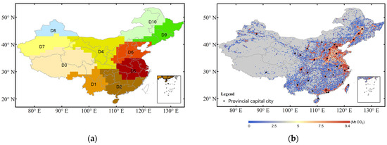
Figure 2.
(a) Clustered areas (subregions) derived from the clustering analysis of spatiotemporal XCO2 using the XCO2 data from 2010 to 2021; (b) anthropogenic CO2 emissions from ODIAC in 2021.
Next, we divided the emissions data into two parts based on the emission intensity thresholds of each subregion. We implemented an iterative operation of extracting the training datasets by changing the threshold to find the optimal threshold with the minimum error of the prediction model. Multiplied training datasets with emission values generated in steps of 100, from 0 to 1000, were used to build the prediction model based on the CatB algorithm. Then, the optimal threshold with the minimum error was found using cross-validation of the multiplied emission prediction results. As a result, when the emission value was set at 200, the prediction error was at its minimum.
Lastly, 20 training datasets in the study area were generated with 2 levels of emission intensities and 10 subregions from the clustering analysis. Hereafter, these datasets are referred to as SubSeg-Sdatasets. These 20 datasets were used for training and learning, respectively, to build the prediction models.
We also extracted the other three training datasets using different methods to compare and evaluate the prediction accuracy and effect of these different datasets. They were (1) only based on the subregions from the clustering of XCO2 above to generate 10 training datasets in the study area (hereafter, referred to as Sub-Sdatasets); (2) only based on the segmenting threshold of emissions to obtain 2 training datasets in the study area (hereafter, referred to as Seg-Sdatasets); and (3) all of the data in this study were used as the training data (hereafter, referred to as One-Sdataset). The training datasets above were from 2019 to 2020, including all the prediction parameters and ODIAC data, as shown in Table 1.
2.2.2. ACE Prediction Modeling and Verification
We selected three integrated complex (boosting) algorithms based on decision tree and gradient boosting (GBDT) algorithms, including LightGBM, XGBoost, and CatBoost, to better evaluate the models based on the different training datasets above. These algorithms can better handle nonlinear problems and are suitable for processing large-scale and high-dimensional feature datasets. They are highly interpretable and can explain the quantitative impact of different parameter features on the prediction results based on their own feature importance and dependency graphs, using tools such as SHAP. The prediction accuracy of LightGBM (LGB) is not better than that of the other two algorithmic frameworks, but it is faster in operation, occupies less memory, and is able to better deal with large datasets under the same hardware conditions [43]. XGBoost (XGB) is not only able to use a decision tree as the base learner but also supports a variety of base learners, including linear learners, which can reduce overfitting bias and improve prediction accuracy [44]. CatBoost (CatB) is based on a fully symmetric tree, which solves the problems of gradient bias and prediction bias and thus can effectively inhibit data overfitting; thus, it has a great advantage in dealing with small datasets (e.g., high emission values) [45]. We compared and analyzed the models and ACE predictions based on these algorithms to determine the most feasible and optimal algorithms out of the three.
The prediction models were built using the training datasets from 2019 to 2020, respectively (SubSeg-Sdatasets, Seg-Sdatasets, Sub-Sdatasets, and One-Sdataset), which were created using the four methods described in Section 2.2 and combined with the three ML algorithms (CatB, LGB, and XGB). For each ML algorithm, the predictions of ACEs were respectively implemented using multiple models from the multiple training datasets of SubSeg-Sdatasets, Sub-Sdatasets, and Seg-Sdatasets in the corresponding areas, while the prediction was implemented using a single model from the One-Sdataset.
The cross-validation dataset, moreover, was extracted by randomly sampling the ODIAC data and the prediction parameter data from 2019 to 2020, and these data were excluded from the training data corresponding to their locations in space and time. The statistical indicators, the goodness-of-fit (R2), the mean absolute error (MAE), and the root-mean-square error (RMSE), were used to verify the models’ accuracy. The ODIAC data in 2021, moreover, were used as the test data to assess the performances of the predicted ACEs and the validity of the prediction models.
3. Results
3.1. Cross-Validation of ML Predictions
In order to verify the model prediction accuracy, we predicted the ACEs using the prediction parameter variables (Mp, including XCO2, NO2, NL, IS, SIF, NDVI, D2M, T2M, U10, V10, and RN) from 2019 to 2020 in the cross-validation datasets and calculated the goodness-of-fit (R2), the root-mean-square error (RMSE), and the mean absolute error (MAE) between the ODIAC data and the prediction results using the cross-validation dataset. Figure 3 shows the results of the cross-validation for each prediction model derived from the combinations of the training datasets (SubSeg-Sdatasets, Seg-Sdatasets, Sub-Sdatasets, and One-Sdataset) and the ML algorithms (CatB, LGB, and XGB).
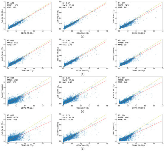
Figure 3.
Cross-validation (CV) of the prediction models based on three algorithms (CatB, LGB, and XGB) from the four sampling methods: (a) SubSeg-Sdatasets; (b) Seg-Sdatasets; (c) Sub-Sdatasets; and (d) One-Sdataset, where the unit of the RMSE and MAE is MtCO2 × 10−4.
As shown in Figure 3, we compared the predicted ACEs from four training datasets (SubSeg-Sdatasets shown in Figure 3a, Seg-Sdatasets shown in Figure 3b, Sub-Sdatasets shown in Figure 3c, and One-Sdataset shown in Figure 3d) using the same ML algorithms with the ODIAC data. The prediction accuracy based on the training using the SubSeg-Sdatasets was better than those from the other three training datasets, demonstrating the best fit with R2 (0.97) and the smallest MAE (3.6 MtCO2 × 10−4) and RMSE (19.56 MtCO2 × 10−4). This result indicates the validity of the model based on SubSeg-Sdatasets, derived from the clustering of XCO2 combined with the division of the anthropogenic emission intensities, indicating it is more likely to achieve unbiased modeling for predicting ACEs. The predicted ACEs from the model based on the One-Sdataset demonstrated the lowest accuracy out of the three ML algorithms, which indicates the effects of the non-normal distribution of ACEs mentioned above.
The different ML algorithms for the predictions have different sensitivities to the sampling methods of the training data. The prediction accuracies based on the CatB and LGB algorithms were significantly improved from the One-Sdataset to the SubSeg-Sdatasets, with the R2 value increasing from 0.69 to 0.97 and from 0.75 to 0.97, respectively, and the RMSE decreasing from 67 to 20 MtCO2 × 10−4 and from 67 to 18 MtCO2 × 10−4, respectively. These results indicate that the model based on the CatB and LGB algorithms is more likely to be impacted by the training samples, depending on the spatial distribution of the emission data. The prediction accuracy based on the XGB algorithm did not significantly change with the sampling method, with the R2 value slightly increasing from 0.84 to 0.95 and the RMSE decreasing from 48 to 24 MtCO2 × 10−4, which shows that the XGB is less sensitive to the effects of different training samples.
It can also be seen in Figure 3a that the MAE (2.43 MtCO2 × 10−4) based on the LGB algorithm was slightly better than the MAE (3.60 MtCO2 × 10−4) based on the CatB under the training of the Sub-Segsdatasets. We further assess and analyze the prediction effects (generalization performance) from the spatial features of biases on the prediction results in 2021 in the next section.
3.2. Performance of ML Algorithms for ACE Prediction
In order to evaluate the generalization performance of each prediction model in space, we predicted the monthly ACEs in 2021 for the whole of the study area and compared the spatial differences with the ODIAC data in the same year. The cross-validation only indicates the accuracy of the prediction model itself.
We applied the prediction parameter dataset in 2021 to predict the monthly ACEs in 2021 using the multiple prediction models, respectively, built by the training datasets (SubSeg-Sdatasets, Seg-Sdatasets, Sub-Sdatasets, and One-Sdataset), combined with the ML algorithms (CatB, LGB, and XGB).
Generally, the evaluation indexes (R2, RMSE, and MAE) of cross comparison between the predicted ACEs and the ODIAC data in 2021 for the entire study area, which are shown in Table 2, indicate that the predicted ACEs derived from the model based on the combinations of the SubSeg-Sdatasets with CatB were still slightly better than the other training datasets and ML algorithms. For the model based on the SubSeg-Sdatasets, the predicted results combined with the CatB (0.96, 22.74 MtCO2 × 10−4, 4.97 MtCO2 × 10−4) present slightly smaller biases than those with the LGB and XGB, while the MAE of the predictions with the LGB was the smallest (2.43 MtCO2 × 10−4) in the cross-validation, as shown in Figure 3.
Table 2.
Comparison of prediction results with ODIAC data in 2021 in the study area.
Figure 4 shows the spatial features of the biases of the predicted ACEs by the four training datasets combined with the CatB, which demonstrated the lowest biases among the three ML algorithms in assessing the generalization performances of the predicted results.
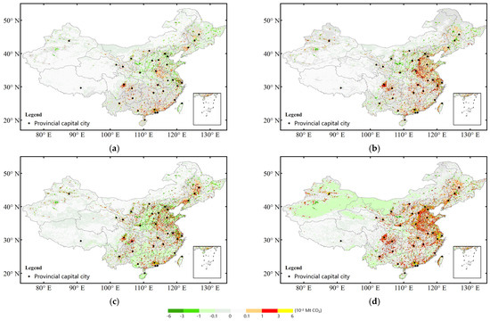
Figure 4.
The biases of predicted ACEs compared to ODIAC modeling based on the four training datasets, (a) SubSeg–Sdatasets, (b) Seg–Sdatasets, (c) Sub–Sdatasets, and (d) One–Sdataset, combined with the CatB algorithm.
It can be seen in Figure 4 that the prediction biases from the SubSeg-Sdatasets model (Figure 4a) were significantly the least in space compared to the other three training dataset models (Figure 4b–d). The SubSeg-Sdatasets better model the predicted ACEs, especially in the high-emission areas of eastern China.
The predicted ACE values from the Seg-Sdatasets, Sub-Sdatasets, and One-Sdataset models were generally higher than the inventory emissions of ODIAC in the high-emission areas. The prediction biases from the One-Sdataset model presented the largest biases in the eastern region. Compared to the spatial variation of the ODIAC, as shown in Figure 2, high biases in the prediction results from the Seg-Sdatasets, Sub-Sdatasets, and One-Sdataset models were significantly concentrated in high-emission areas, such as the big cities in China, and economically developed areas, such as the Beijing–Tianjin–Hebei area and the Yangtze River Delta. These results indicate that these three training datasets are insufficient to address the issue of the non-normal distribution of ACEs due to too many samples with low ACE values and few samples with intermediate and high ACE values, resulting in poor training and learning of the prediction model.
Furthermore, we compared the predictive effectiveness of the three ML algorithms based on the training of SubSeg-Sdatasets, as they presented similar cross-validations, as shown in Figure 3. Figure 5 presents the biases of the predicted ACEs and their correspondence with the emission intensities from the ODIAC data for the CatB, LGB, and XGB models with the SubSeg–Sdatasets.
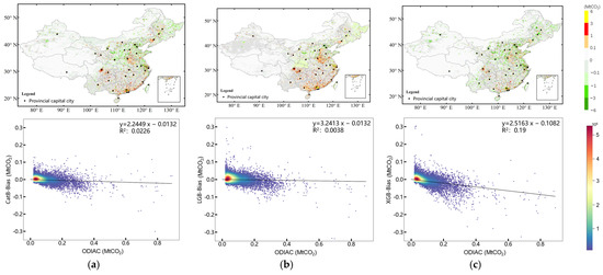
Figure 5.
Prediction biases and scatterplots of prediction biases corresponding to ODIAC for each grid in 2021 from the three ML algorithms ((a) CatB, (b) LGB, and (c) XGB) with the SubSeg–datasets.
Figure 5 illustrates the linear correlation between the ODIAC value and the deviation (estimation result–ODIAC value). A lower R2 value indicates a more accurate estimation result, while an R2 of 0 signifies no deviation between the ODIAC and the estimation result. It can be seen in Figure 5 that the predicted result using XGB modeling was slightly lower than that using CatB, while the XGB generally presented a slight linear trend with the ODIAC data. This result indicates that predictions from the XGB modeling are likely to have systematic biases, which implies that the prediction models are mostly constrained by some variables with a linear relationship to anthropogenic emissions. The average predicted ACEs from the XGB were lower than those from the CatB for the entire study area (see Figure S1a). The mean prediction bias based on the XGB model, however, was −0.1074 MtCO2, with high ODIAC values ranging from 0.6 to 0.8 MtCO2, which was larger than the bias based on the CatB (−0.0381 MtCO2) (see Figure S1a) due to low predictions in the high-emission sources from the XGB modeling.
4. Discussion
The data-driven method based on machine learning to predict the ACEs could apply lots of predictor parameters to constrain the prediction model of ACEs affected by various factors. The previous study, which is similar to our study, also applied machine learning models to predict ACEs for the year 2019 using a stacked random forest regression model derived using XCO2, NL, NDVI, and terrestrial CO2 flux data from 2014 to 2018 as the predictor parameters [27]. That study validated and discussed the predicting results at the national scale, where the predicted ACE for the Chinese region was 6.5% lower than ODIAC in 2019 and did not demonstrate the reasonableness of the spatial distribution of predicted ACEs in detail. Our prediction of ACEs, with the Chinese region as the study area, is 6% higher than ODIAC in 2021, and we evaluated the validity of the data-driven method to determine whether the predicted results accurately reveal the spatial characteristics of ACEs in China. We would extend the study areas, such as the American land area, to validate our proposed approach in the future. Another additional study built the grid-based prediction model by the generalized regression neural network (GRNN) algorithm using a long time series of data from 2010 to 2019, each grid including XCO2 and SIF, where the predicted ACE was 4% lower than ODIAC in 2019 for the Chinese region and indicated that larger predicting biases were mainly located around the big cities [28]. This GRNN model needs long-term series data that are difficult to collect when using multiple parameters, which could not further improve the prediction accuracy of the model. Our study introduces multiple parameters up to 11 variables (XCO2, NO2, NL, IS, SIF, NDVI, D2M, T2M, U10, V10, and RN), which are helpful to improve the accuracy of the prediction model.
All the predictor variables used in this study were from satellite observations. The number of predictor variables used in this study, moreover, was higher than that in previous studies, and the NL predictor variable was also used as a proxy in the ODIAC.
We applied the SHAP method to calculate and visualize the ranking of the total contribution of each parameter to the predictions for the CatB, LGB, and XGB models based on the SubSeg-Sdatasets, which is shown in Figure 6.
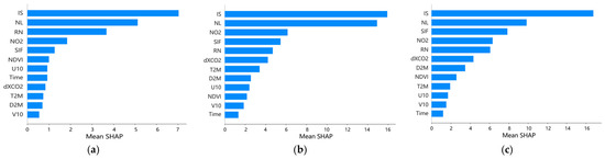
Figure 6.
SHAP values (average impact on model magnitude) of the contributions of the prediction parameters to predictions based on the SubSeg-Sdatasets, combined with (a) CatB modeling, (b) LGB modeling, and (c) XGB modeling.
The results show that impervious surfaces (IS) and nighttime lighting (NL) ranked as the top contributors to the predictions in the three algorithms, which indicates a strong relationship between the IS and NL parameters, revealing the relationship between urbanization, human activities, and anthropogenic CO2 emissions (see Figure S2 also). This is consistent with the findings of Rahman et al. [46]. The high contributions of IS and NL could also be because ODIAC uses NL, point sources of emissions, and population data as proxies in the production methodology of ODIAC’s inventory to generate spatial grid data based on the national total emission statistics. There are also emission point sources and populations in the IS areas.
The contribution of the atmospheric parameter XCO2 to the predictions of the XGB model was higher than that of the CatB model, indicating that the XGB model is likely to increase the contributions of atmospheric parameters to ACEs. Therefore, the XGB could compress the signal of point source emissions over impervious surfaces, which would result in low prediction in these areas, as shown in Figure S1b. The prediction accuracy and performance using XGB modeling were similar to those using CatB modeling (Figure 3 and Figure 5), but the contributions of the prediction parameters were different, as shown in Figure 6a,c), where the SHAP values of XCO2 were larger in the XGB than in the CatB. The XGB model could be more accurate than the CatB model, as the XGB model is more constrained by the CO2 concentration, which corresponds to the changes in the ACEs [32,33]. However, the XGB showed low predictions from the high-emission sources, which could be because of the CO2 constraint, where ODIAC overestimated the emissions, which needs to be explored further.
NO2 emissions are mainly from fossil fuel combustion, and thus, a strong correlation of 0.63 was shown between the ODIAC data and NO2 (see Figure S2). It is known that CO2 emissions are generally accompanied by NO2 emissions. The grid distribution of the statistical emissions from the ODIAC data is only based on the surface characteristic parameters and does not consider the atmospheric parameters, like NO2, which strongly affect anthropogenic CO2 emissions. A prediction model that introduces the atmospheric NO2 parameter could reduce some of the uncertainty of the ODIAC emissions in the spatial redistribution.
We introduced satellite-based XCO2 as a predictor variable, as well as variables related to terrestrial ecology (SIF and NDVI) and atmospheric transport (ERA5), since atmospheric CO2 originates from anthropogenic emissions, terrestrial ecology, and atmospheric transport. The SHAP values showed that the ecological parameters SIF and NDVI contributed to the prediction more than the dXCO2, and the meteorological variables (U10, V10, T2M, and D2M) also showed SHAP values of 0.5–1, which implies that the effects of ecological vegetation fluxes and transport fluxes are included in XCO2.
Lastly, we also made predictions using different combinations of the predictor parameters using the CatB model based on the SubSeg-Sdatasets. The cross-validation of the results indicates that the prediction using all of the parameters as input was still the optimal method. The parameters of IS and RN, which were high contributors to the predictions, tended to affect the prediction of dynamic ACEs, as they were the static variables. The spatial biases of the predicted ACEs could be increased by these static variables, smoothing the changes in the ACEs. Therefore, we should add dynamic emission sources and mobile transport emissions from impervious surfaces and roads to modeling predictions in the future.
5. Conclusions
In the process of modeling predictions based on machine learning, extracting training sample data used for the training and learning of the prediction model is an important step to assure the accuracy and optimal performance of the prediction. Appropriate sampling methods for the training data to resolve the issue of the non-normal distribution of ACEs can significantly improve the prediction performance of the model. Accordingly, we proposed a sampling method based on the clustering of the spatiotemporal characteristics of XCO2 combined with the division of emissions to extract the training datasets (SubSeg-Sdatasets). Moreover, we also needed to find an ML algorithm that could accurately drive the prediction model using the training datasets. Respectively, we implemented the prediction model using combinations of the four training datasets (SubSeg-Sdatasets, Sub-Sdatasets, Seg-Sdatasets, and One-Sdataset) and the three ML algorithms (CatB, LGB, and XGB) using multiple parameters (XCO2, NO2, NL, IS, SIF, NDVI, D2M, T2M, U10, V10, and RN) as the predictor variables and ODIAC as the predicted variable. We evaluated the model’s prediction accuracy using cross-validation and the performance of the predicted results.
As a result, the predictions from the CatB and LGB models combined with the SubSeg-Sdatasets were slightly better than those from the XGB based on cross-validation, whereas the predictions based on CatB modeling and XGB modeling demonstrated better predictive effectiveness when analyzing the prediction performances in spatial biases and the overall statistics of ACEs in the study area. We found that it was not enough to verify the prediction using cross-validation alone; we needed to explore the prediction bias characteristics in detail using the performance of the predicted results to reveal the spatial characteristics of the ACEs accurately.
Satellite-based data have the advantage of being stable and objective observations. Predicting anthropogenic CO2 emissions using satellite data based on machine learning modeling, on the one hand, can be applied to monitor and evaluate anthropogenic CO2 emissions as a top-down measure. On the other hand, it can be compared with the ODIAC data, which are only based on the static parameters of the surface characteristics and do not include atmospheric parameters. The approach proposed in this study introduces the dynamic observations of atmospheric NO2 and CO2, which suggests that a data-driven prediction of anthropogenic CO2 emissions can supplement the shortage of proxies used in generating ODIAC data. Moreover, satellite observations can help us obtain anthropogenic CO2 emissions data earlier than inventory emissions data, with the advantages of their near-real-time and high-coverage observations. By using these data, anthropogenic CO2 emission prediction modeling based on machine learning has great application potential as a supplement to and in comparison with emission inventory data.
In the future, the combination of machine learning and mechanistic modeling is expected to improve the estimation of ACEs, and the combination of mechanistic modeling can help us to interpret the results theoretically.
Supplementary Materials
The following supporting information can be downloaded at: https://www.mdpi.com/article/10.3390/atmos15030323/s1, Table S1: Summary of abbreviations; Figure S1: Comparison of average predicted ACEs in 2021 based on the four training datasets (SubSeg–Sdatasets, Seg–Sdatasets, Sub–Sdatasets, One–Sdataset) combined with three ML algorithms (CatB, LGB, XGB) and ODIAC in the study area; Figure S2: Heat map of the correlations among variables.
Author Contributions
Conceptualization, H.S. and L.L.; validation, Z.J. and L.L.; writing—original draft, Z.J.; data curation, H.S.; methodology, Z.J. and H.S.; software, M.S., S.Z. and K.G. All authors have read and agreed to the published version of the manuscript.
Funding
This research was funded by the National Key Research and Development Program of China (grant no. 2022YFC3800700) and the National Key Research and Development Program of China (grant no. 2020YFA0607503).
Institutional Review Board Statement
Not applicable.
Informed Consent Statement
Not applicable.
Data Availability Statement
The research data presented in this study are available on request from the corresponding author. The data are not publicly available due to this project is still in the research phase.
Acknowledgments
We are very grateful to the Center for Global Environmental Research, National Institute for Environmental Studies for providing the ODIAC2022 version of the dataset, available from doi:10.17595/20170411.001 (accessed on 29 January 2024). We thank the European Space Agency (ESA) and Google Earth Engine for providing Sentinel-S5P NO2 products and the ERA5 dataset produced by the Copernicus Climate Change Service (C3S) at ECMWF. Thanks to the National Aeronautics and Space Administration (NASA) for sharing NDVI data obtained from MODIS and nighttime light data downloaded from https://eogdata.mines.edu/products/vnl/ (accessed on 29 January 2024). We also thank Xiao’s Global Ecology Group for producing the GOSIF dataset, which is available at the Global Ecology Data Repository.
Conflicts of Interest
The authors declare no conflicts of interest. The China Highway Engineering Consultants Corporation had no role in the design of the study; in the collection, analyses, or interpretation of data; in writing of the manuscript, or in the decision to publish results.
References
- Olivier, J.G.; Schure, K.M.; Peters, J.A.H.W. Trends in Global CO2 and Total Greenhouse Gas Emissions; PBL Netherlands Environmental Assessment Agency: The Hague, The Netherlands, 2017; Volume 5, pp. 1–11. [Google Scholar]
- Yuan, W.; Cai, W.; Chen, Y.; Liu, S.; Dong, W.; Zhang, H.; Yu, G.; Chen, Z.; He, H.; Guo, W.; et al. Severe Summer Heatwave and Drought Strongly Reduced Carbon Uptake in Southern China. Sci. Rep. 2016, 6, 18813. [Google Scholar] [CrossRef]
- Philippe, C.; Christopher, S.; Govindasamy, B.; Bopp, L.; Victor, B.; Josep, C.; Abha, C.; Ruth, D.; James, G.; Heimann, M.; et al. Carbon and Other Biogeochemical Cycles. In Climate Change 2013: The Physical Science Basis. Contribution of Working Group I to the Fifth Assessment Report of the Intergovernmental Panel on Climate Change; Cambridge University Press: Cambridge, UK, 2014; pp. 465–570. [Google Scholar]
- Masson-Delmotte, V.P.; Zhai, P.; Pirani, S.L.; Connors, C.; Péan, S.; Berger, N.; Caud, Y.; Chen, L.; Goldfarb, M.I.; Scheel Monteiro, P.M. IPCC, 2021: Summary for policymakers. In Climate Change 2021: The Physical Science Basis. Contribution of Working Group to the Sixth Assessment Report of the Intergovernmental Panel on Climate Change; Cambridge University Press: Cambridge, UK; New York, NY, USA, 2021; pp. 3–32. [Google Scholar]
- Duren, R.M.; Miller, C.E. Towards Robust Global Greenhouse Gas Monitoring. Greenh. Gas Meas. Manag. 2011, 1, 80–84. [Google Scholar] [CrossRef]
- Abdullah, L.; Pauzi, H.M. Methods in forecasting carbon dioxide emissions: A decade review. J. Teknol. 2015, 75, 67–82. [Google Scholar] [CrossRef]
- Le Quéré, C.; Andrew, R.M.; Canadell, J.G.; Sitch, S.; Korsbakken, J.I.; Peters, G.P.; Manning, A.C.; Boden, T.A.; Tans, P.P.; Houghton, R.A.; et al. Global Carbon Budget 2016. Earth Syst. Sci. Data 2016, 8, 605–649. [Google Scholar] [CrossRef]
- Andres, R.J.; Boden, T.A.; Higdon, D. A New Evaluation of the Uncertainty Associated with CDIAC Estimates of Fossil Fuel Carbon Dioxide Emission. Tellus B Chem. Phys. Meteorol. 2014, 66, 23616. [Google Scholar] [CrossRef]
- Hutchins, M.G.; Colby, J.D.; Marland, G.; Marland, E. A Comparison of Five High-Resolution Spatially-Explicit, Fossil-Fuel, Carbon Dioxide Emission Inventories for the United States. Mitig. Adapt. Strateg. Glob. Chang. 2017, 22, 947–972. [Google Scholar] [CrossRef]
- Andrew, R.M. A Comparison of Estimates of Global Carbon Dioxide Emissions from Fossil Carbon Sources. Earth Syst. Sci. Data 2020, 12, 1437–1465. [Google Scholar] [CrossRef]
- Andres, R.J.; Boden, T.A.; Higdon, D.M. Gridded Uncertainty in Fossil Fuel Carbon Dioxide Emission Maps, a CDIAC Example. Atmos. Chem. Phys. 2016, 16, 14979–14995. [Google Scholar] [CrossRef]
- Gaughan, A.E.; Oda, T.; Sorichetta, A.; Stevens, F.R.; Bondarenko, M.; Bun, R.; Krauser, L.; Yetman, G.; Nghiem, S.V. Evaluating Nighttime Lights and Population Distribution as Proxies for Mapping Anthropogenic CO2 Emission in Vietnam, Cambodia and Laos. Environ. Res. Commun. 2019, 1, 091006. [Google Scholar] [CrossRef]
- Han, P.; Zeng, N.; Oda, T.; Lin, X.; Crippa, M.; Guan, D.; Janssens-Maenhout, G.; Ma, X.; Liu, Z.; Shan, Y.; et al. Evaluating China’s Fossil-Fuel CO2 Emissions from a Comprehensive Dataset of Nine Inventories. Atmos. Chem. Phys. 2020, 20, 11371–11385. [Google Scholar] [CrossRef]
- Jonas, M.; Bun, R.; Nahorski, Z.; Marland, G.; Gusti, M.; Danylo, O. Quantifying Greenhouse Gas Emissions. Mitig. Adapt. Strateg. Glob. Chang. 2019, 24, 839–852. [Google Scholar] [CrossRef]
- Belgiu, M.; Drăguţ, L. Random Forest in Remote Sensing: A Review of Applications and Future Directions. ISPRS J. Photogramm. Remote Sens. 2016, 114, 24–31. [Google Scholar] [CrossRef]
- Tramontana, G.; Jung, M.; Schwalm, C.R.; Ichii, K.; Camps-Valls, G.; Ráduly, B.; Reichstein, M.; Arain, M.A.; Cescatti, A.; Kiely, G.; et al. Predicting Carbon Dioxide and Energy Fluxes across Global FLUXNET Sites with Regression Algorithms. Biogeosciences 2016, 13, 4291–4313. [Google Scholar] [CrossRef]
- Chevallier, F.; Broquet, G.; Zheng, B.; Ciais, P.; Eldering, A. Large CO2 Emitters as Seen From Satellite: Comparison to a Gridded Global Emission Inventory. Geophys. Res. Lett. 2022, 49, e2021GL097540. [Google Scholar] [CrossRef]
- Kumari, S.; Singh, S.K. Machine Learning-Based Time Series Models for Effective CO2 Emission Prediction in India. Environ. Sci. Pollut. Res. 2023, 30, 116601–116616. [Google Scholar] [CrossRef]
- Li, Z. The CO2 Emission Forecasting in Asia in Context of Time-Series and Machine Learning Approaches. In Proceedings of the Second International Conference on Statistics, Applied Mathematics, and Computing Science (CSAMCS 2022), Nanjing, China, 28 March 2023; Jin, S., Dai, W., Eds.; SPIE: Nanjing, China, 2023; p. 141. [Google Scholar]
- Li, X.; Zhang, X. A Comparative Study of Statistical and Machine Learning Models on Carbon Dioxide Emissions Prediction of China. Environ. Sci. Pollut. Res. 2023, 30, 117485–117502. [Google Scholar] [CrossRef]
- Radojević, D.; Pocajt, V.; Popović, I.; Perić-Grujić, A.; Ristić, M. Forecasting of Greenhouse Gas Emissions in Serbia Using Artificial Neural Networks. Energy Sources Part A Recovery Util. Environ. Eff. 2013, 35, 733–740. [Google Scholar] [CrossRef]
- Liu, P.; Zhang, G.; Zhang, X.; Cheng, S. Carbon Emissions Modeling of China Using Neural Network. In Proceedings of the 2012 Fifth International Joint Conference on Computational Sciences and Optimization, Harbin, China, 23–26 June 2012; IEEE: Harbin, China, 2012; pp. 679–682. [Google Scholar]
- Yap, W.K.; Karri, V. Emissions Predictive Modelling by Investigating Various Neural Network Models. Expert Syst. Appl. 2012, 39, 2421–2426. [Google Scholar] [CrossRef]
- Behrang, M.A.; Assareh, E.; Assari, M.R.; Ghanbarzadeh, A. Using Bees Algorithm and Artificial Neural Network to Forecast World Carbon Dioxide Emission. Energy Sources Part A Recovery Util. Environ. Eff. 2011, 33, 1747–1759. [Google Scholar] [CrossRef]
- Li, S.; Zhou, R.; Ma, X. The Forecast of C02 Emissions in China Based on RBF Neural Networks. In Proceedings of the 2010 2nd International Conference on Industrial and Information Systems, Dalian, China, 10–11 July 2010; Volume 1, pp. 319–322. [Google Scholar]
- Mustafa, F.; Bu, L.; Wang, Q.; Yao, N.; Shahzaman, M.; Bilal, M.; Aslam, R.W.; Iqbal, R. Neural-Network-Based Estimation of Regional-Scale Anthropogenic CO2 Emissions Using an Orbiting Carbon Observatory-2 (OCO-2) Dataset over East and West Asia. Atmos. Meas. Tech. 2021, 14, 7277–7290. [Google Scholar] [CrossRef]
- Zhang, Y.; Liu, X.; Lei, L.; Liu, L. Estimating Global Anthropogenic CO2 Gridded Emissions Using a Data-Driven Stacked Random Forest Regression Model. Remote Sens. 2022, 14, 3899. [Google Scholar] [CrossRef]
- Zhang, S.; Lei, L.; Sheng, M.; Song, H.; Li, L.; Guo, K.; Ma, C.; Liu, L.; Zeng, Z. Evaluating Anthropogenic CO2 Bottom-Up Emission Inventories Using Satellite Observations from GOSAT and OCO-2. Remote Sens. 2022, 14, 5024. [Google Scholar] [CrossRef]
- Richardson, K.; Steffen, W.; Lucht, W.; Bendtsen, J.; Cornell, S.E.; Donges, J.F.; Drüke, M.; Fetzer, I.; Bala, G.; von Bloh, W.; et al. Earth beyond Six of Nine Planetary Boundaries. Sci. Adv. 2023, 9, eadh2458. [Google Scholar] [CrossRef]
- Oda, T.; Maksyutov, S.; Andres, R.J. The Open-Source Data Inventory for Anthropogenic CO2, Version 2016 (ODIAC2016): A Global Monthly Fossil Fuel CO2 Gridded Emissions Data Product for Tracer Transport Simulations and Surface Flux Inversions. Earth Syst. Sci. Data 2018, 10, 87–107. [Google Scholar] [CrossRef]
- Oda, T.; Maksyutov, S. A Very High-Resolution (1 Km×1 Km) Global Fossil Fuel CO2 Emission Inventory Derived Using a Point Source Database and Satellite Observations of Nighttime Lights. Atmos. Chem. Phys. 2011, 11, 543–556. [Google Scholar] [CrossRef]
- Yang, S.; Lei, L.; Zeng, Z.; He, Z.; Zhong, H. An Assessment of Anthropogenic CO2 Emissions by Satellite-Based Observations in China. Sensors 2019, 19, 1118. [Google Scholar] [CrossRef]
- Sheng, M.; Lei, L.; Zeng, Z.-C.; Rao, W.; Song, H.; Wu, C. Global Land 1° Mapping Dataset of XCO2 from Satellite Observations of GOSAT and OCO-2 from 2009 to 2020. Big Earth Data 2023, 7, 170–190. [Google Scholar] [CrossRef]
- Van der A, R.J.; Eskes, H.J.; Boersma, K.F.; van Noije, T.P.C.; Van Roozendael, M.; De Smedt, I.; Peters, D.H.M.U.; Meijer, E.W. Trends, Seasonal Variability and Dominant NOx Source Derived from a Ten Year Record of 2 Measured from Space. J. Geophys. Res. Atmos. 2008, 113, e2007JD009021. [Google Scholar] [CrossRef]
- Sheng, M.; Lei, L.; Zeng, Z.-C.; Rao, W.; Zhang, S. Detecting the Responses of CO2 Column Abundances to Anthropogenic Emissions from Satellite Observations of GOSAT and OCO-2. Remote Sens. 2021, 13, 3524. [Google Scholar] [CrossRef]
- van Geffen, J.; Eskes, H.; Compernolle, S.; Pinardi, G.; Verhoelst, T.; Lambert, J.-C.; Sneep, M.; ter Linden, M.; Ludewig, A.; Boersma, K.F.; et al. Sentinel-5P TROPOMI NO2 Retrieval: Impact of Version v2.2 Improvements and Comparisons with OMI and Ground-Based Data. Atmos. Meas. Tech. 2022, 15, 2037–2060. [Google Scholar] [CrossRef]
- Li, X.; Xiao, J. A Global, 0.05-Degree Product of Solar-Induced Chlorophyll Fluorescence Derived from OCO-2, MODIS, and Reanalysis Data. Remote Sens. 2019, 11, 517. [Google Scholar] [CrossRef]
- Cao, L.; Chen, X.; Zhang, C.; Kurban, A.; Yuan, X.; Pan, T.; De Maeyer, P. The Temporal and Spatial Distributions of the Near-Surface CO2 Concentrations in Central Asia and Analysis of Their Controlling Factors. Atmosphere 2017, 8, 85. [Google Scholar] [CrossRef]
- Liiv, J.; Ivar, Z.; Tämm, K.; Rikmann, E. Greenhouse Gases Emissions and Climate Change beyond Mainstream. MOJ Biorg. Org. Chem. 2020, 4, 11–16. [Google Scholar]
- Meng, L.; Graus, W.; Worrell, E.; Huang, B. Estimating CO2 (Carbon Dioxide) Emissions at Urban Scales by DMSP/OLS (Defense Meteorological Satellite Program’s Operational Linescan System) Nighttime Light Imagery: Methodological Challenges and a Case Study for China. Energy 2014, 71, 468–478. [Google Scholar] [CrossRef]
- Shan, Y.; Guan, D.; Zheng, H.; Ou, J.; Li, Y.; Meng, J.; Mi, Z.; Liu, Z.; Zhang, Q. China CO2 Emission Accounts 1997–2015. Sci. Data 2018, 5, 170201. [Google Scholar] [CrossRef]
- Zhang, X.; Liu, L.; Wu, C.; Chen, X.; Gao, Y.; Xie, S.; Zhang, B. Development of a Global 30 m Impervious Surface Map Using Multisource and Multitemporal Remote Sensing Datasets with the Google Earth Engine Platform. Earth Syst. Sci. Data 2020, 12, 1625–1648. [Google Scholar] [CrossRef]
- Ke, G.; Meng, Q.; Finley, T.; Wang, T.; Chen, W.; Ma, W.; Ye, Q.; Liu, T.-Y. LightGBM: A Highly Efficient Gradient Boosting Decision Tree. In Proceedings of the Proceedings of the 31st International Conference on Neural Information Processing Systems, Red Hook, NY, USA, 4 December 2017; Curran Associates Inc.: Red Hook, NY, USA, 2017; pp. 3149–3157. [Google Scholar]
- Chen, T.; Guestrin, C. XGBoost: A Scalable Tree Boosting System. In Proceedings of the 22nd ACM SIGKDD International Conference on Knowledge Discovery and Data Mining, New York, NY, USA, 13 August 2016; Association for Computing Machinery: New York, NY, USA, 2016; pp. 785–794. [Google Scholar]
- Prokhorenkova, L.; Gusev, G.; Vorobev, A.; Dorogush, A.V.; Gulin, A. CatBoost: Unbiased Boosting with Categorical Features. In Proceedings of the 32nd International Conference on Neural Information Processing Systems, Red Hook, NY, USA, 3 December 2018; Curran Associates Inc.: Red Hook, NY, USA, 2018; pp. 6639–6649. [Google Scholar]
- Rahman, M.M.; Shafiullah, M.; Alam, M.S.; Rahman, M.S.; Alsanad, M.A.; Islam, M.M.; Islam, M.K.; Rahman, S.M. Decision Tree-Based Ensemble Model for Predicting National Greenhouse Gas Emissions in Saudi Arabia. Appl. Sci. 2023, 13, 3832. [Google Scholar] [CrossRef]
Disclaimer/Publisher’s Note: The statements, opinions and data contained in all publications are solely those of the individual author(s) and contributor(s) and not of MDPI and/or the editor(s). MDPI and/or the editor(s) disclaim responsibility for any injury to people or property resulting from any ideas, methods, instructions or products referred to in the content. |
© 2024 by the authors. Licensee MDPI, Basel, Switzerland. This article is an open access article distributed under the terms and conditions of the Creative Commons Attribution (CC BY) license (https://creativecommons.org/licenses/by/4.0/).