Short-Term Probabilistic Wind Speed Predictions Integrating Multivariate Linear Regression and Generative Adversarial Network Methods

Abstract

The precise forecasting of wind speeds is critical to lessen the harmful impacts of wind fluctuations on power networks and aid in merging wind energy into the grid system. However, prior research has predominantly focused on point forecasts, often overlooking the uncertainties inherent in the prediction accuracy. For this research, we suggest a new approach for forecasting wind speed intervals (PI). Specifically, the actual wind speed series are initially procured, and the complete ensemble empirical mode decomposition coupled with adaptive noise (CEEMDAN) method decomposes the actual wind speed series into constituent numerous mode functions. Furthermore, a generative adversarial network (GAN) is utilized to achieve the wind speed PI in conjunction with the multivariate linear regression method. To confirm the effectiveness of the suggested model, four datasets are selected. The validation results suggest that this suggested model attains a superior PI accuracy compared with those of numerous benchmark techniques. In the context of PI of dataset 4, the PINAW values show improvements of 68.06% and 32.35% over the CEEMDAN-CNN and VMD-GRU values in single-step forecasting, respectively. In conclusion, the proposed model excels over the counterpart models by exhibiting diminished a PINAW and CWC, while maintaining a similar PICP.

1. Introduction

In the context of climate change, marked by the increase in the global mean temperature, the earth is experiencing amplified occurrences of extreme climatic events, such as thunderstorms, floods, and typhoons [1,2]. The mitigation of carbon emissions has emerged as a critical global target, with numerous nations committing to this objective. Wind power, a sustainable energy resource, has been increasingly adopted on a global scale [3,4]. However, the inherent variability and intermittency of wind patterns raise substantial challenges to the efficient harnessing and exploitation of wind energy. Therefore, precise wind speed prediction (WSP) techniques are crucial to guarantee the risk-free functioning and seamless planning of wind energy systems. This has spurred a plethora of research efforts to improve the performance of WSP.

In the realm of short-term WSP, numerous methodologies exist, which are broadly recognized as physical techniques [5,6,7], statistical methods [8,9,10], and artificial intelligence (AI) techniques [11,12]. Physical models often rely on solving the equations of fluid motion (e.g., numerical weather forecasting), which can lead to inaccuracies for the short-term forecasting results. Statistical methods, on the other hand, construct predictive models based on an abundant quantity of wind velocity records, but the prediction effects on nonlinear data are still unsatisfactory.

Nowadays, AI-based approaches have gained considerable traction. Various AI-based models have been developed and implemented for definite or probabilistic WSP purposes [13,14,15,16]. For example, Liu et al. [17] and Ruiz-Aguilar et al. [18] conduct wind speed predictions with ELM (Extreme Learning Machine) and ANN (Artificial Neural Network), respectively. Liu et al. [19] and Memarzadeh et al. [20] both use long short-term memory (LSTM) neural network for wind speed forecasting. Despite the progress, multiple difficulties continue to impede the wide usage of these AI-driven methodologies. Initially, the natural unpredictability of the “original state” in climatic tendencies, attributable to their intensely nonlinear character, presents a considerable obstacle in judging the value of predictive ambiguities. Additionally, time-lapse data on wind speed houses intricate atmospheric particulars, necessitating copious training data for sufficient detail extraction. Finally, separate models of neural networks have their distinct scenarios for optimal application, which can restrict their resilience in diverse situations.

Recent scholarly endeavors have focused on the innovative fusion of diverse benchmark models to develop a hybrid model with superior forecasting performances, a technique referred to ensemble methods [21]. Two primary categories can segregate Ensemble Forecasting Methods (EFMs): the Competing Ensemble Predictive Approach (CmEPA) and Cooperating Ensemble Predictive Approach (CpEPA) [22]. CmEPA fuses related prediction models into one coordinated ensemble model; in contrast, CpEPA employs assorted independent units, maintaining reciprocal communication. Contrasted with CmEPA, CpEPA often offers a better forecasting accuracy of wind speed and exhibits a wider range of research domains. The CpEPA frameworks encompass data selection, feature decomposition, optimization algorithm, and result postprocessing [23,24]. Capitalizing on the EFM, a multitude of studies have embarked on deterministic and probabilistic WSP. The objective of these endeavors aims to augment the precision of deterministic wind speed forecasting. A substantial body of literature corroborates that the EFM outperforms the individual models in the context of WSP performance [25,26]. Taking the feature decomposition for example, Hu et al. [27] and Wang et al. [28] both employ ensemble empirical mode decomposition with adaptive noise (CEEMDAN) for wind speed forecasting.

The task of probabilistic short-term wind speed forecasting continues to present significant challenges, warranting further exploration due to the intricate uncertainties inherent in the meteorological systems. In this study, we construct an innovative CpEPA designed specifically for short-term WSP. In particular, we utilize the complete ensemble empirical mode decomposition coupled with the adaptive noise (CEEMDAN) technique for wind speed series decomposition. Afterward, the generative adversarial network (simplified as GAN, comprising a bi-directional gate recurrent unit network (BIGRU) generator and convolutional neural network (CNN) discriminator) is applied to train the decomposed subseries for wind speed interval prediction (PI). Lastly, to assess the robustness of the suggested combined approach (abbreviated as CGBIG), a comparative analysis is conducted between our suggested model and the other fundamental models for wind speed PI (utilizing four time series wind speed datasets). Compared to the currently existing research, the main contributions in this study are presented as follows: wind speed PI is conducted, integrating the multivariate line regression theory with a generative adversarial network (GAN, a promising and powerful forecasting model).

The ensuing configuration is set up below. Section 2 offers a concise overview for theoretical foundations related to the methods used in the proposed hybrid models. Subsequent to this, Section 3 carries out case study analysis to confirm the efficacy of the suggested model. In the end, Section 4 houses the conclusions.

2. Theory Descriptions of Related Methods

A novel hybrid model is proposed in this study (called CGBIG), and the flowchart of the proposed model is presented in Figure 1. In this part, theory descriptions of the related methods for the proposed model are depicted as follows.

2.1. CEEMDAN Method

Ensemble Empirical Modal Decomposition (EEMD) [29] incorporates noise that is not completely eliminated during the decomposition process, resulting in large reconstruction errors. Therefore, CEEMDAN is proposed, which reduces the number of iterations and improves the accuracy of the reconstructed signal. The steps of CEEMDAN are as follows:

Step 1: For initial time series signals denoted x(t), noise is incorporated, which is calculated below.

$${\mathrm{x}}^k(t)=\mathrm{x}(t)+\sigma {\gamma }^k(t)$$

(1)

where σ denotes random values with the standard normal distribution; γ^k(t) (k = 1, 2, 3, …, K) corresponds to varying instances of white Gaussian noise.

Step 2: The EMD decomposition [30] of each set of signals is performed to obtain the first intrinsic modal component (IMF). Then, the residual signal component of the first decomposition is obtained. The formulas are expressed as follows:

$$IM{F}_1\left(t\right)=\frac{1}{K}{\displaystyle \sum _1^{K}IM{F}_1^k\left(t\right)}$$

(2)

$$r_1(t)=\mathrm{x}(t)-IM{F}_1\left(t\right)$$

(3)

Step 3: The above two steps are repeated to obtain the i-th IMF component and corresponding residuals R(t), which are presented as follows:

$$R\left(t\right)=\mathrm{x}(t)-{\displaystyle \sum _{i=1}^{I}IM{F}_i\left(t\right)}$$

(4)

where I is the number of decompositions.

2.2. GAN Model

The GAN paradigm, a prominent unsupervised framework, comprises two principal components, namely, the discriminator (D) and the generator (G). Within the GAN framework, the iterative interplay between these models engenders the generation of predictive outputs, ultimately converging towards Nash equilibrium [31,32]. In our research, we introduce these two models (G and D), denoted as BIGRU and CNN, respectively, in the ensuing exposition.

2.2.1. Discriminative Model: CNN

The discriminative model in our study adopts the CNN approach, an intricate multi-tiered, feed-forward artificial NN (neural network). Notably, the CNN offers distinct advantages including sparse connectivity and weight sharing, enabling it to delve into the extraction of intricate data features with a reduced count of model parameters [33,34]. In this work, the CNN architecture comprises three convolutional strata and a pair of layers that is fully interconnected. A comprehensive overview of this architectural configuration of each layer within the CNN model is presented in

Table 1. Structures of the discriminative model—CNN.

CNN Configuration s from D Model
Conv1D	filter counts	128
	kernel sizes	2
	activation function	LeakyRelu
Conv1D	filter counts	256
	kernel sizes	2
	activation function	LeakyRelu
Conv1D	filter counts	512
	kernel sizes	2
	activation function	LeakyRelu
Dense	units	256
	activation function	relu

.

2.2.2. Generative Model-BIGRU

In the realm of time series analysis, the Bi-directional Gated Recurrent Unit (BIGRU) stands out as a compelling alternative, especially when contrasted with the other variants of recurrent NN (e.g., long short-term memory) [35,36]. Notably, the BIGRU exhibits a proclivity for rapid convergence and economic benefits in terms of the model parameters. This streamlined attribute imparts a simplified network structure and bolsters the operational efficiency, all while preserving the predictive performance. Consequently, the BIGRU presents itself as an option that is both simpler and more effective in addressing time series analysis challenges [37]. It is particularly adept at capturing the intricate nonlinear relationships inherent in time series data, rendering it a favored choice for resolving pertinent time series problems [38]. Compared with the GRU, the BIGRU is effective in capturing temporal correlation whether originating from past or future data, and the BIGRU structures in this paper are presented in

Table 2. Parameter settings of the GAN-BIGRU model.

Model	Parameters	Quantity
GAN-BIGRU	Quantity of GRU layers	3
	Count of neurons within GRU layers	128, 256, 512
	Size of the batch	4
	Optimization method	adam

. Detailed calculation formulas are presented below.

$$r_t=\sigma \left(w_{\mathrm{rs}}{S}_{t-1}+w_{\mathrm{rx}}{X}_{rt}+b_{\mathrm{rsx}}\right)$$

(5)

$$z_{\mathrm{t}}=\sigma \left(w_{\mathrm{zs}}{S}_{t-1}+w_{\mathrm{zx}}{X}_{\mathrm{t}}+b_{zsx}\right)$$

(6)

$${\tilde{S}}_t=\tan \mathrm{h}\left[w_{\mathrm{ss}}\left(r_t\odot S_{t-1}\right)+w_{\mathrm{hx}}{X}_t\right]$$

(7)

$$S_t=\left(1-z_t\right)\odot {\tilde{S}}_t+z_t\odot S_{t-1}$$

(8)

where σ is sigmoid function; S_t and S_t−1 represent the hidden state at moments t and t − 1, respectively; $\odot$ symbolizes the Hadamard multiplying factor; and w and b denote the weights and biases, respectively.

2.3. Interval Prediction Theory

Within the realm of regression issues, the pursuit to approximate an undisclosed function, marked as f(x; θ), becomes critical when faced with a succession of input pairs, denoted as B = {x_i, t_i} (i = 1, 2, …, m). Here, φ symbolizes the actual parameters of the regression approach, and n represents the dataset size. Equation (1) clarifies the functional correlation between the elusive g(x; φ) and actual values t.

$$ti=\mathrm{g}(xi;\phi )+ei$$

(9)

where e_i is the error in the model, obeying the N (0, σ²) distribution with the variance denoted by σ². The estimation of φ, represented as $\widehat{\phi }$, involves the minimization of the following objective function C(φ):

$$C(\phi )={\displaystyle {\sum }_{i=1}^n{(t_i-y_i)}^2}$$

(10)

$$y_i=g(x_i;\widehat{\phi })$$

(11)

where y_i signifies output of the model. In the event that the regression model assumes a multivariate and linear form, Equation (3) is reformulated below.

$$y_i={\widehat{\beta }}_0+{\widehat{\beta }}_1{x}_1+\cdots +{\widehat{\beta }}_i{x}_i$$

(12)

where ${\widehat{\beta }}_0$, ${\widehat{\beta }}_1$, $\cdots$, ${\widehat{\beta }}_i$ encompass the parameters of the regression approach.

Leveraging the assumption of Gaussian distribution, wherein the model error follows a zero mean and σ standard deviation, we can derive the (1 − α) PI confidence (PINC) level using the subsequent formula.

$$L_i=y_i-B$$

(13)

$$U_i=y_i+B$$

(14)

where $U_i$ and $L_i$ signify the upper and lower limits for the i-th PI. B represents the limit or margin of error, computed using the following formula:

$$B=z_{\alpha /2}\sigma =z_{\alpha /2}\widehat{\sigma }\sqrt{(1+{x_i}^T{(X^{T}X)}^{-1}{x}_i)}$$

(15)

where the matrix X depicts the input space, x_i is the i-th row within X matrix. s is deemed the unbiased approximation of σ (the value of freedom degrees equaling n − p), which is given as follows:

$$s=\sqrt{\frac{1}{(n-p-1)}{\displaystyle \sum _{i=1}^n{(t_i-y_i)}^2}}$$

(16)

where p signifies the parameters’ number.

2.4. Performance Evaluation Indices

To appraise the superiority of the recommended model as well as the benchmark techniques, three assessment metrics are employed: the coverage probability of PI (PICP), the coverage width-based criterion (CWC), and the PI normalized average width (PINAW). These three metrics are calculated as shown below.

$$PICP=\frac{1}{N}{\displaystyle {\sum }_{i=1}^N{v}_i}$$

(17)

$$PINAW=\frac{1}{N}{\displaystyle {\sum }_{i=1}^N\frac{U_i-L_i}{y_{\max }-y_{\min }}}$$

(18)

$$CWC=\left\{\begin{array}{l}PINAW(1+e^{(-\eta (PICP-\mu ))}),\mathrm{PICP}\text{<}\mu \\ PINAW,\mathrm{PICP}\ge \mu \end{array}\right.$$

(19)

where c_i assumes a value of 1 if y_t falls within the prediction interval. Conversely, v_i takes on the value of 0 when y_t lies outside the PI. Notably, the bounds of the PI are defined, signifying the maximum values (y_max) and minimum values (y_min) within the test set, respectively. Additionally, $\mu$ designates the level of PINC, a parameter of significance in quantifying the accuracy of the prediction intervals. It is pertinent to mention that the value of $\eta$ is established as 50, based on recent references [39].

3. Case Studies

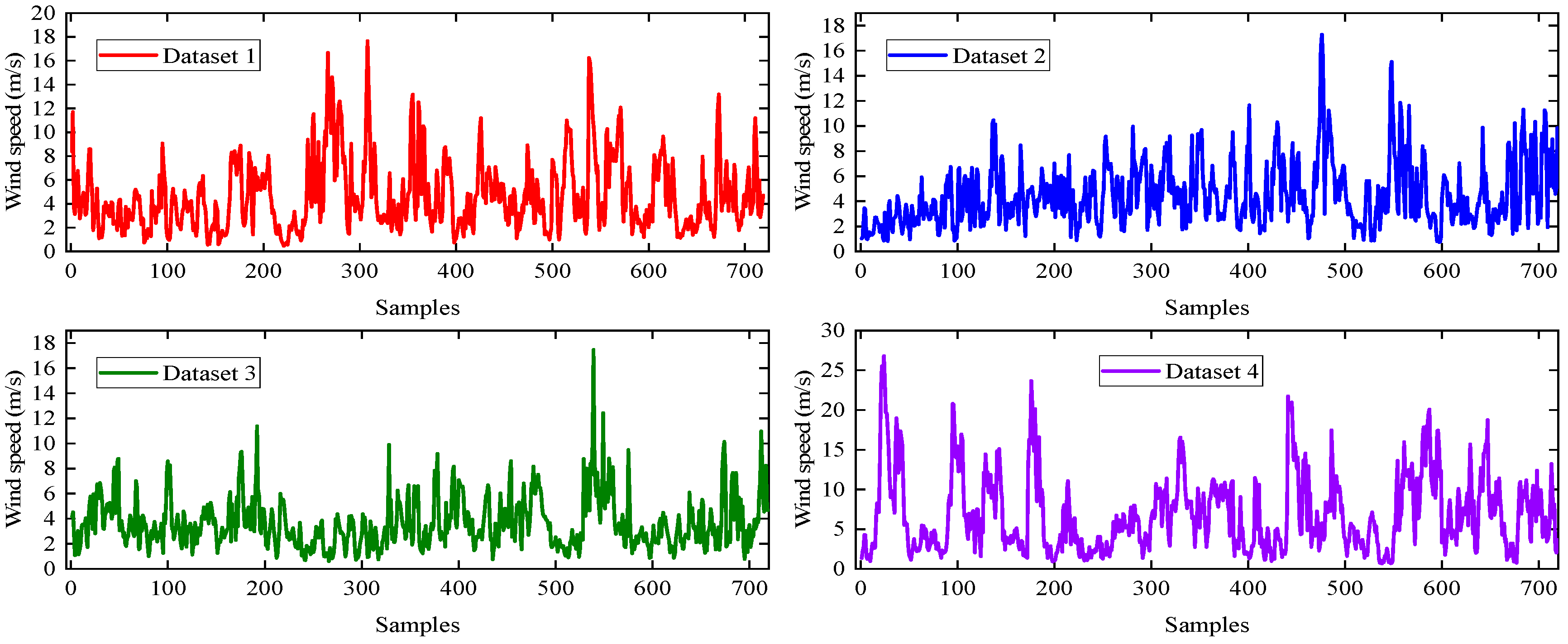
3.1. Data Collection

For this study, the dataset under scrutiny is procured from a climatological tower situated to the west of Colorado (39.9106° N, 105.2347° W). As per the authorized web portal [40], it is possible to acquire wind speed data at hourly intervals. Furthermore, in an effort to confirm the stability of the suggested model, we chose several datasets from distinct months (March, June, September, and December of 2022), each symbolizing the typical seasons of spring, summer, fall, and winter. The aforementioned datasets are depicted in Figure 2. Moreover, the first 80% is used as the training set, and the rest is used for the test set.

3.2. Short-Term Probabilistic WSP

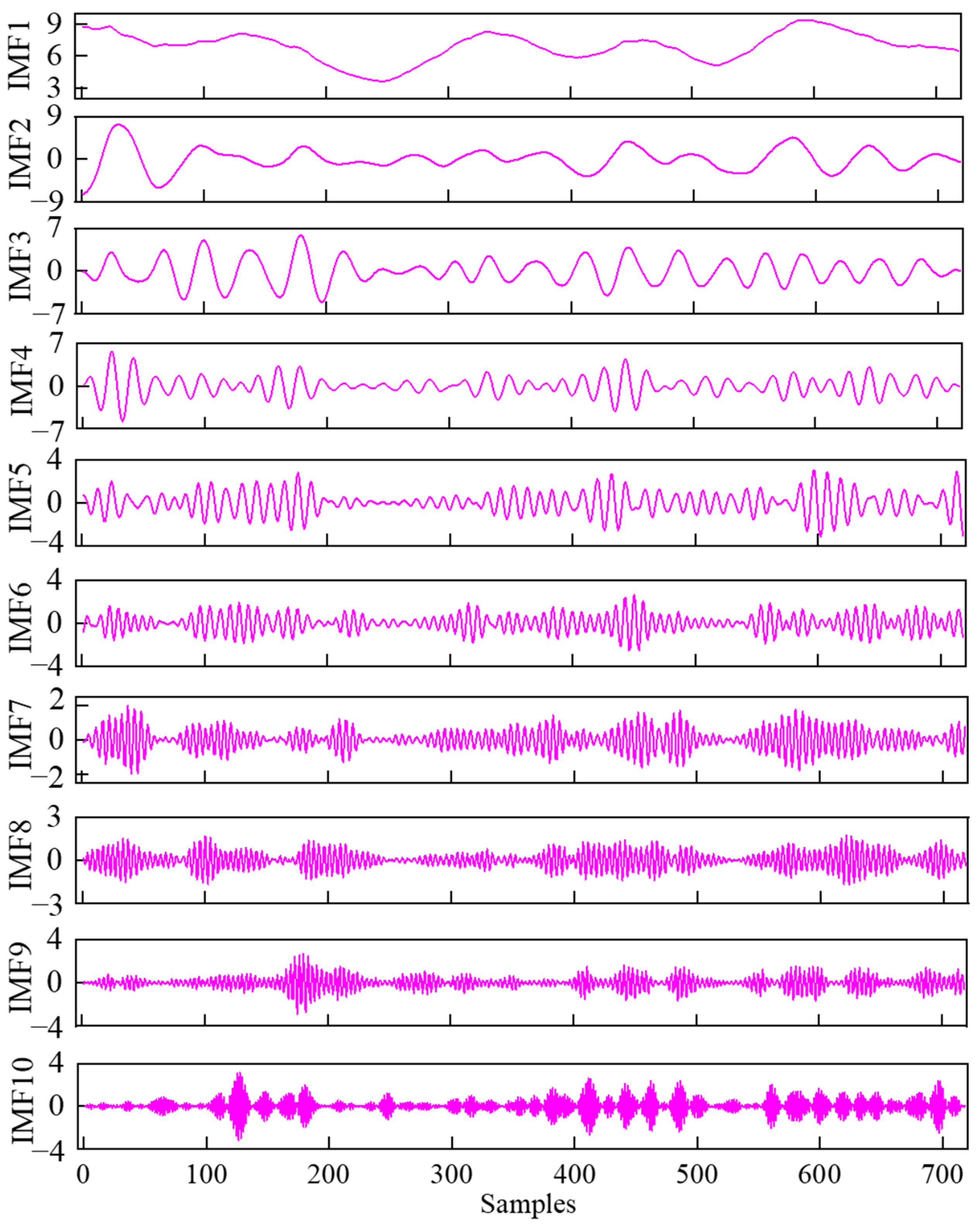
3.2.1. Decomposition Results of the CEEMDAN Method

The model under consideration, referred to as CGBIG, is employed for PI of the 1 h mean wind speeds. Initially, the wind speed datasets (derived from Section 3.1) are subjected to the CEEMDAN method to eliminate the trend terms inherent in the datasets, thereby reducing the randomness of the wind speeds. This process, in turn, enhances the Predictive Interval (PI) forecasting performances. Given the constraints on the length of this article, we have chosen to present the decomposition results of a single dataset (1 h mean wind speed from March 2022), which are illustrated in Figure 3.

3.2.2. The Results of Single-Step and Multi-Step Interval Predictions

In this section, we delineate the outcomes of single-step interval predictions derived from the proposed approach and other benchmark techniques (such as CEEMDAN-BIGRU, CEEMDAN-GRU, and CEEMDAN-CNN) when α is set to 0.05. Figure 4 illustrates the Predictive Interval (PI) outcomes of these four models for dataset 4. Additionally, we juxtapose the results of evaluation metrics for single-step and multi-step interval predictions (two, five, and seven steps) derived from these four models, as exhibited in

Table 3. Results of evaluation metrics among these four methods.

Models	Datasets	Single-Step			Two-Step
		PICP	PINAW	CWC	PICP	PINAW	CWC
CEEMDAN-CNN	Dataset1	1	0.562	0.562	1	0.582	0.582
	Dataset2	1	0.543	0.543	1	0.630	0.630
	Dataset3	1	0.554	0.554	1	0.576	0.576
	Dataset4	1	0.432	0.432	1	0.450	0.450
CEEMDAN-GRU	Dataset1	1	0.261	0.261	1	0.335	0.335
	Dataset2	1	0.260	0.260	1	0.338	0.338
	Dataset3	1	0.217	0.217	1	0.286	0.286
	Dataset4	1	0.204	0.204	1	0.268	0.268
CEEMDAN-BIGRU	Dataset1	1	0.258	0.258	1	0.330	0.330
	Dataset2	1	0.257	0.257	1	0.320	0.320
	Dataset3	1	0.201	0.201	1	0.285	0.285
	Dataset4	1	0.189	0.189	1	0.261	0.261
The proposed model	Dataset1	1	0.186	0.186	1	0.251	0.251
	Dataset2	1	0.149	0.149	1	0.262	0.262
	Dataset3	1	0.151	0.151	1	0.221	0.221
	Dataset4	1	0.138	0.138	1	0.207	0.207
Model	Dataset	Five-step			Seven-step
		PICP	PINAW	CWC	PICP	PINAW	CWC
CEEMDAN-CNN	Dataset1	1	0.745	0.745	1	0.841	0.841
	Dataset2	1	0.758	0.758	1	0.864	0.864
	Dataset3	1	0.719	0.719	1	0.797	0.797
	Dataset4	1	0.576	0.576	1	0.683	0.683
CEEMDAN-GRU	Dataset1	1	0.557	0.557	1	0.685	0.685
	Dataset2	1	0.573	0.573	1	0.696	0.696
	Dataset3	1	0.469	0.469	1	0.588	0.588
	Dataset4	1	0.481	0.481	1	0.617	0.617
CEEMDAN-BIGRU	Dataset1	1	0.535	0.535	1	0.671	0.671
	Dataset2	1	0.549	0.549	1	0.695	0.695
	Dataset3	1	0.461	0.461	1	0.571	0.571
	Dataset4	1	0.469	0.469	1	0.576	0.576
The proposed model	Dataset1	1	0.447	0.447	1	0.564	0.564
	Dataset2	1	0.464	0.464	1	0.604	0.604
	Dataset3	1	0.388	0.388	1	0.503	0.503
	Dataset4	1	0.392	0.392	1	0.507	0.507

. We emphasize that the hyper-parameterizations of the benchmark techniques mirror those of the suggested approach (as detailed in Table 1 and Table 2). From Figure 4 and Table 3, we can infer the following conclusions:

(1)

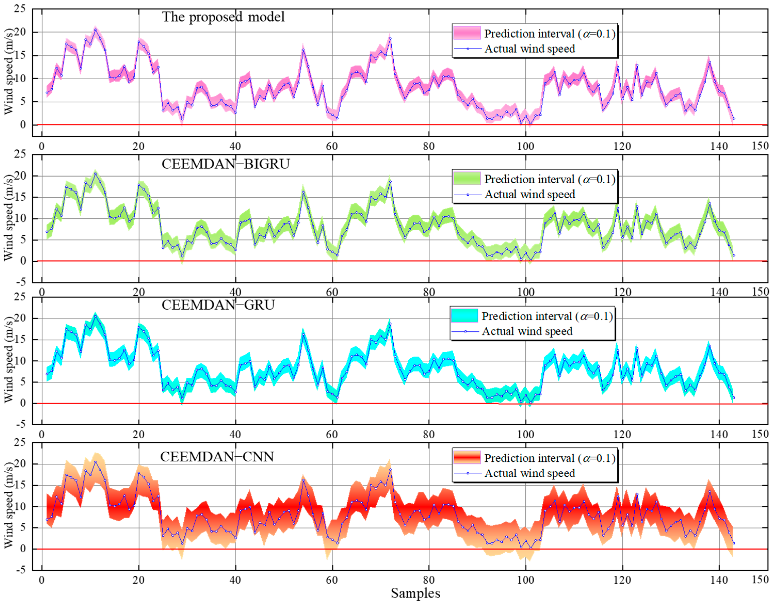
It is readily apparent that these four models yield accurate interval predictions, with a PICP value of one across these four datasets. For instance, considering dataset 4, the CEEMDAN-CNN model exhibits the highest PINAW, with a value of 0.432. This implies that this model provides the least accurate PI compared to the other three models, as clearly depicted in Figure 3. Furthermore, the predicting accuracy of the CEEMDAN-BIGRU surpasses that of the CEEMDAN-GRU, and the forecasting accuracies of these two models are both inferior to that from the suggested model, presenting PINAWs of 0.38, 0.189, and 0.204 in respective order.

(2)

In terms of the CWC, the suggested approach significantly outperforms the other analogous techniques, owing to its minimal CWC. This outcome is anticipated as the suggested model maintains a minimal PINAW and comparable or even superior PICP. Relative to the CEEMDAN-CNN, the CWC shows an enhancement of 68.06% in single-step interval forecasting for dataset 4. When compared with the other two models, the CWC values of the suggested model consistently remain the smallest. Similar conclusions can be drawn for multi-step interval forecasting. In conclusion, upon reviewing each performance indicator, the proposed approach outshines the rival standard approaches in individual as well as sequential interval projections. The reason is that the proposed model consists of two models (discriminative model—CNN; generative model—BIGRU), and combines the strengths of these two models. Additionally, compared with the GRU, the BIGRU is effective in capturing temporal correlation, whether originating from past or future data. Therefore, the proposed model performs better than the other benchmark models.

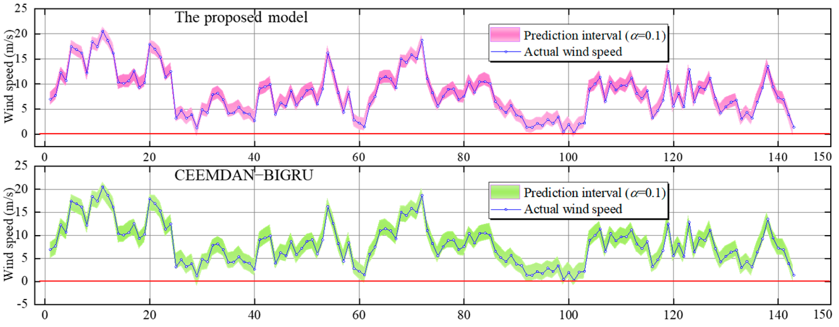
3.3. Verification of Distribution Estimation

Section 3.2 demonstrates the superiority of the recommended approach over the three benchmark techniques when α is set to 0.05. In this section, we extend our investigation to other quantiles (α = 0.1) to further substantiate the pre-eminence of the suggested model. This implies that the suggested model enables to estimate the entire forecasting distribution. As seen from the comparative experiment analysis in Section 3.2, the performance of the CEEMDAN-BIGRU surpasses that of the other two models (CEEMDAN-GRU and CEEMDAN-CNN). Consequently, the predictive results are compared with those obtained by the CEEMDAN-BIGRU for α = 0.1. Figure 5 depicts the resulting prediction intervals of these two models for the fourth dataset when α is designated as 0.1. Various assessment measurements are recorded in

Table 4. Contrasting measurement of evaluation metrics on multiple datasets (α = 0.1).

α = 0.1	Datasets	PICP	PINAW	CWC
CEEMDAN-BIGRU	Dataset1	1	0.218	0.218
	Dataset2	1	0.220	0.220
	Dataset3	1	0.191	0.191
	Dataset4	1	0.169	0.169
The proposed model	Dataset1	1	0.122	0.122
	Dataset2	1	0.148	0.148
	Dataset3	1	0.135	0.135
	Dataset4	1	0.127	0.127

. By analyzing Figure 5 and Table 4, it is evident that due to the smaller PINAW with the CWC measurements, the recommended model consistently excels over the VMD-GRU.

4. Conclusions

In this study, we introduce a novel model designed to execute prediction interval based on a deep learning methodology and multivariate linear regression theory. Furthermore, four datasets verify the effectiveness of the suggested approach in individual and successive predicting tasks. Grounded on the predictive results and contrasting investigation, the key deductions can be concluded as follows:

(1)

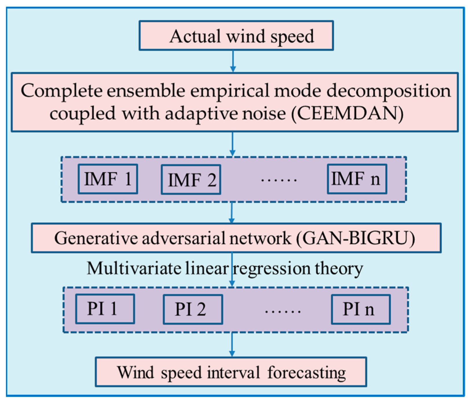
A novel generative adversarial network (GAN) enhanced by CEEMDAN is suggested to achieve the PI for wind speed grounded in the multivariate linear regression theory. This suggested model is adept at accurately capturing the randomness in wind speed and quantifying and reducing the uncertainty of forecasting outcomes.

(2)

The operation of the suggested approach for both single-stage and multiple-stage projections is confirmed through the utilization of four datasets. When concerning interval predictions of dataset 4, the PINAW values of the recommended model are disclosed as 0.138 and 0.127 for diverse PINC quantities of 0.95 and 0.9 in single-step prediction in a respective manner.

(3)

The experimental outcomes suggest that the operation of the suggested model excels the over relative techniques because of its reduced PINAW with CWC values, all the while maintaining identical PICP values. Fundamentally, it creates PIs that encapsulate the unpredictability in the wind speed forecasting.

This study introduces a new technique for PI that additionally assesses the variation range in wind speed projections. Such hybrid methods are beneficial for risk analysis and the evaluation of wind speed series by decision makers in power systems. However, there are various wind events with distinct wind characteristics. Therefore, the recommended method’s efficiency in predicting various wind types necessitates a more detailed exploration. Moreover, the effects of the wind azimuth and direction on the prediction accuracy have been ignored and will be studied in our future work.

References

1. Sadorsky, P. Wind energy for sustainable development: Driving factors and future outlook. J. Clean. Prod. 2021, 289, 125779. [Google Scholar] [CrossRef]
2. Wang, Y.; Hu, Q.; Li, L.; Foley, A.M.; Srinivasan, D. Approaches to wind power curve modeling: A review and discussion. Renew. Sustain. Energy Rev. 2019, 116, 109422. [Google Scholar] [CrossRef]
3. Zhao, X.Y.; Liu, J.F.; Yu, D.R.; Chang, J.T. One-day-ahead probabilistic wind speed forecast based on optimized numerical weather prediction data. Energy Convers. Manag. 2018, 164, 560–569. [Google Scholar] [CrossRef]
4. Landberg, L. Short-term prediction of the power production from wind farms. J. Wind. Eng. Ind. Aerod. 1999, 80, 207–220. [Google Scholar] [CrossRef]
5. Miguel, Á.P.F.; Carlos-Otero, C.; Felipe, C.F.; Gonzalo, M.M. Wind power forecasting for a real onshore wind farm on complex terrain using WRF high resolution simulations. Renew. Energy 2019, 135, 674–686. [Google Scholar]
6. Zhao, J.; Guo, Y.; Xiao, X.; Wang, J.; Chi, D.; Guo, Z. Multi-step wind speed and power forecasts based on a WRF simulation and an optimized association method. Appl. Energy 2017, 197, 183–202. [Google Scholar] [CrossRef]
7. Chen, K.; Yu, J. Short-term wind speed prediction using an unscented Kalman filter based state-space support vector regression approach. Appl. Energy 2014, 113, 690–705. [Google Scholar] [CrossRef]
8. Guo, Z.; Zhao, J.; Zhang, W.; Wang, J. A corrected hybrid approach for wind speed prediction in Hexi Corridor of China. Energy 2011, 36, 1668–1679. [Google Scholar] [CrossRef]
9. Cassola, F.; Burlando, M. Wind speed and wind energy forecast through Kalman filtering of Numerical Weather Prediction model output. Appl. Energy 2012, 99, 154–166. [Google Scholar] [CrossRef]
10. Khosravi, A.; Koury, R.N.N.; Machado, L.; Pabon, J.J.G. Prediction of wind speed and wind direction using artificial neural network, support vector regression and adaptive neuro-fuzzy inference system. Sustain. Energy Technol. Assess. 2018, 25, 146–160. [Google Scholar] [CrossRef]
11. Liu, H.; Tian, H.Q.; Pan, D.F.; Li, Y.F. Forecasting models for wind speed using wavelet, wavelet packet, time series and Artificial Neural Networks. Appl. Energy 2013, 107, 191–208. [Google Scholar] [CrossRef]
12. Kong, X.; Liu, X.; Shi, R.; Lee, K.Y. Wind speed prediction using reduced support vector machines with feature selection. Neurocomputing 2015, 169, 449–456. [Google Scholar] [CrossRef]
13. Saeed, A.; Li, C.S.; Gan, Z.H.; Xie, Y.Y.; Liu, F.J. A simple approach for short-term wind speed interval prediction based on independently recurrent neural networks and error probability distribution. Energy 2022, 238, 122012. [Google Scholar] [CrossRef]
14. Zhang, Y.G.; Pan, G.F.; Zhao, Y.P.; Li, Q.; Wang, F. Short-term wind speed interval prediction based on artificial intelligence methods and error probability distribution. Energy Convers. Manag. 2020, 224, 113346. [Google Scholar] [CrossRef]
15. Wang, J.Z.; Cheng, Z.S. Wind speed interval prediction model based on variational mode decomposition and multi-objective optimization. Appl. Soft Comput. 2021, 113, 107848. [Google Scholar] [CrossRef]
16. Liu, H.; Mi, X.W.; Li, Y.F. An experimental investigation of three new hybrid wind speed forecasting models using multi-decomposing strategy and ELM algorithm. Renew. Energy 2018, 123, 694–705. [Google Scholar] [CrossRef]
17. Liu, Z.Y.; Hara, R.; Kita, H. Hybrid forecasting system based on data area division and deep learning neural network for short-term wind speed forecasting. Energy Convers. Manag. 2021, 238, 114136. [Google Scholar] [CrossRef]
18. Ruiz-Aguilar, J.J.; Turias, I.; González-Enrique, J.; Urda, D.; Elizondo, D. A permutation entropy-based EMD-ANN forecasting ensemble approach for wind speed prediction. Neural Comput. Appl. 2021, 33, 2369–2391. [Google Scholar] [CrossRef]
19. Liu, H.; Yu, C.; Wu, H.; Duan, Z.; Yan, G. A new hybrid ensemble deep reinforcement learning model for wind speed short term forecasting. Energy 2020, 202, 117794. [Google Scholar] [CrossRef]
20. Memarzadeh, G.; Keynia, F. A new short-term wind speed forecasting method based on fine-tuned LSTM neural network and optimal input sets. Energy Convers. Manag. 2020, 213, 112824. [Google Scholar] [CrossRef]
21. Xiang, L.; Li, J.X.; Hu, A.J.; Zhang, Y. Deterministic and probabilistic multi-step forecasting for short-term wind speed based on secondary decomposition and a deep learning method. Energy Convers. Manag. 2020, 220, 113098. [Google Scholar] [CrossRef]
22. Xiang, H.Y.; Zhang, M.J. Data mining-assisted short-term wind speed forecasting by wavelet packet decomposition and Elman neural network. J. Wind. Eng. Ind. Aerod. 2018, 175, 136–143. [Google Scholar]
23. Zhang, L.F.; Wang, J.Z.; Niu, X.S.; Liu, Z.K. Ensemble wind speed forecasting with multi-objective Archimedes optimization algorithm and sub-model selection. Appl. Energy 2021, 301, 117449. [Google Scholar] [CrossRef]
24. Ding, W.; Meng, F.Y. Point and interval forecasting for wind speed based on linear component extraction. Appl. Soft. Comput. 2020, 93, 106350. [Google Scholar] [CrossRef]
25. Sun, W.; Tan, B.; Wang, Q.Q. Multi-step wind speed forecasting based on secondary decomposition algorithm and optimized back propagation neural network. Appl. Soft Comput. 2021, 113, 107894. [Google Scholar] [CrossRef]
26. Zhang, G.W.; Liu, D. Causal convolutional gated recurrent unit network with multiple decomposition methods for short-term wind speed forecasting. Energy Convers. Manag. 2020, 226, 113500. [Google Scholar] [CrossRef]
27. Hu, C.; Zhao, Y.; Jiang, H.; Jiang, M.; You, F.; Liu, Q. Prediction of ultra-short-term wind power based on CEEMDAN-LSTM-TCN. Energy Rep. 2022, 8, 483–492. [Google Scholar] [CrossRef]
28. Wang, S.X.; Shi, J.R.; Yang, W.; Yin, Q.Y. High and low frequency wind power prediction based on Transformer and BiGRU-Attention. Energy 2024, 288, 129753. [Google Scholar] [CrossRef]
29. Wang, S.; Zhang, N.; Wu, L.; Wang, Y. Wind speed forecasting based on the hybrid ensemble empirical mode decomposition and GA-BP neural network method. Renew. Energy 2016, 94, 629–636. [Google Scholar] [CrossRef]
30. Zhang, C.; Wei, H.; Zhao, J.; Liu, T.; Zhu, T.; Zhang, K. Short-term wind speed forecasting using empirical mode decomposition and feature selection. Renew. Energy 2016, 96, 727–737. [Google Scholar] [CrossRef]
31. Goodfellow, I.J.; Pouget-Abadie, J.; Mirza, M.; Xu, B.; Warde-Farley, D.; Ozair, S.; Courville, A.; Bengio, Y. Generative adversarial nets. Adv. Neural Inf. Process. Syst. 2014, 2, 2672–2680. [Google Scholar]
32. Yuan, R.; Wang, B.; Mao, Z.X.; Watada, J. Multi-objective wind power scenario forecasting based on PG-GAN. Energy 2021, 226, 120379. [Google Scholar] [CrossRef]
33. Zhang, Y.M.; Wang, H. Multi-head attention-based probabilistic CNN-BiLSTM for day-ahead wind speed forecasting. Energy 2023, 278, 127865. [Google Scholar] [CrossRef]
34. Zhu, X.X.; Liu, R.Z.; Chen, Y.; Gao, X.X.; Wang, Y.; Xu, Z.X. Wind speed behaviors feather analysis and its utilization on wind speed prediction using 3D-CNN. Energy 2021, 236, 121523. [Google Scholar] [CrossRef]
35. Yu, M.; Niu, D.X.; Gao, T.; Wang, K.K.; Sun, L.J.; Li, M.Y.; Xu, X.M. A novel framework for ultra-short-term interval wind power prediction based on RF-WOA-VMD and BiGRU optimized by the attention mechanism. Energy 2023, 269, 126738. [Google Scholar] [CrossRef]
36. Fanta, H.; Shao, Z.W.; Ma, L.Z. SiTGRU: Single-tunnelled gated recurrent unit for abnormality detection. Inf. Sci. 2020, 524, 15–32. [Google Scholar] [CrossRef]
37. Zhu, T.; Wang, W.B.; Yu, M. A novel hybrid scheme for remaining useful life prognostic based on secondary decomposition, BiGRU and error correction. Energy 2023, 276, 127565. [Google Scholar] [CrossRef]
38. Meng, F.; Song, T.; Xu, D.Y.; Xie, P.F.; Li, Y. Forecasting tropical cyclones wave height using bidirectional gated recurrent unit. Ocean. Eng. 2021, 234, 108795. [Google Scholar] [CrossRef]
39. Khosravi, A.; Nahavandi, S.; Creighton, D.; Atiya, A.F. Lower upper bound estimation method for construction of neural network-based prediction intervals. IEEE Trans. Neural Networks 2011, 22, 337–346. [Google Scholar] [CrossRef]
40. Jager, D.; Andreas, A. NREL National Wind Technology Center (NWTC): M2 Tower; Boulder, Colorado (Data); NREL Report No. DA-5500-56489; National Renewable Energy Laboratory (NREL): Golden, CO, USA, 1996. [Google Scholar]
Figure 1. Flowchart of the proposed model.
Atmosphere 15 00294 g001
Figure 2. Four actual wind speed series used in this paper (datasets 1, 2, 3, and 4).
Atmosphere 15 00294 g002
Figure 3. Results of CEEMDAN decomposition for actual wind speed (dataset 4).
Atmosphere 15 00294 g003
Figure 4. Forecasting interval results of these four methods for dataset 4 using single-step prediction (α = 0.05).
Atmosphere 15 00294 g004
Figure 5. Forecasting interval results of these four methods for dataset4 in single-step predictions (α = 0.1).
Atmosphere 15 00294 g005