Abstract
Accurate monitoring of air pollution is crucial to human health and the global environment. In this research, the various multispectral satellite data, including MODIS AOD/SR, Landsat 8 OLI, and Sentinel-2, together with the two most commonly used machine-learning models, viz. multi-layer backpropagation neural network (MLBPN) and random forest (RF), have been employed to analyze the spatiotemporal distributions of the primary air pollutant from 2019 to 2022 in Guanzhong Region, China. In the conducted experiments, the RF-based model, using the MODIS AOD data, has generally demonstrated the “optimal” estimation performance for the ground-surface concentrations of the primary air-pollutants. Then, the “optimal” estimation model has been employed to analyze the spatiotemporal distribution of the various air pollutants—in terms of temporal distribution, the annual average concentrations of PM2.5, PM10, NO2, and SO2 in the research area showed a decreasing trend from 2019 to 2022, while the annual average concentration of CO remained relatively stable and the annual average concentration of O3 slightly increased; in terms of the spatial distribution, the air pollution presents a gradual increase from west to east in the research area, with the distribution of higher concentrations in the center of the built-up areas and lower in the surrounding rural areas. The proposed estimation model and spatiotemporal analysis can provide reliable methodologies and data support for the further study of the air pollution characteristics in the research area.
1. Introduction
The swift progression of the global economy, coupled with rapid urban expansion and escalating industrial production, has amplified the strain on the atmospheric environment. The consequential atmospheric pollution can not only disrupt the delicate balance of ecosystems and contribute to global climate change but can also pose significant risks to human health [1]. The traditional ground-based observation methods are only able to provide a limited amount of station monitoring data, which cannot comprehensively represent the characteristics regarding the continuous spatial distribution and the temporal changing trends of the primary air pollutants in expansive spatial areas. Characterized by their high timeliness, extensive coverage, and superior resolution, satellite remote-sensing technologies have emerged as a promising solution to compensate for the limitations of the ground-monitoring methods, which have thereby increasingly been leveraged for monitoring atmospheric pollution.
Previous research has mainly relied on limited ground-based monitoring station data and geographic information system (GIS) technology to obtain the spatial distribution of air pollutants. Guo et al. [2] analyzed the temporal–spatial variation characteristics of six air pollutants in 366 major cities in China from 2015 to 2017 using data on the daily average mass concentrations of air pollutants monitored at about 1500 stations published by the Ministry of Environmental Protection (MEP). Han et al. [3] analyzed the spatiotemporal variations in PM2.5 in South Korea among 49 pollution events by using Kriging interpolation and statistical analyses based on the observations from 462 air quality monitoring stations (AQMS) in South Korea from 2015 to 2020. Wang et al. [4] utilized the air pollutant concentration data from 23 monitoring stations in Nanchang City from 2017 to 2020 and obtained the spatial distribution maps of air pollutants by Kriging interpolation to explore the spatiotemporal changes in urban air pollution. However, the limited monitoring stations and spatial coverage make it difficult to depict the spatial distribution of air pollutants comprehensively and accurately. Since the 1960s, with the continuous development of satellite remote-sensing technology, some scholars have begun to use this technology to study the spatial distribution of air pollutants. Yuan et al. [5] analyzed the aerosol spatiotemporal distribution characteristics of Hangzhou using the moderate-resolution imaging spectroradiometer (MODIS) 3 km AOD products from 2012 to 2020, and found that MODIS AOD data can be used as an important basis for atmospheric studies in Hangzhou.
Aerosol research is a critical aspect of advancing contemporary atmospheric quality monitoring technology. Aerosol optical depth (AOD) serves as a measure of aerosol extinction in the vertical direction, closely linked to near-surface atmospheric particulate matter [6,7]. Wang et al. [8] studied the relationship between column aerosol optical thickness (AOT) and PM2.5 mass in the United States and demonstrated that MODIS AOT can be used quantitatively to estimate air quality. Engel-Cox et al. [9] conducted correlation research on MODIS AOD and ground-based particulate matter concentration values at urban and regional scales and found that the correlations of MODIS AOD with ground-based particulate matter were better. Su et al., Qin et al., and Zhang et al. found that fine particulate matter concentration correlated more strongly with AOD through statistical modelling of satellite-observed aerosol optical thickness data and ground-based particulate matter observations, with a better estimation accuracy [10,11,12]. Meanwhile, considering that AOD can be estimated from top-of-atmosphere reflectance (TOA), some researchers have proposed to utilize TOA to estimate PM2.5 concentration directly and proved its effectiveness and applicability [13,14]. Satellite estimation of air pollution fundamentally revolves around establishing the spectral information–pollutant concentration relationship. Directly employing reflectance data for atmospheric pollutant estimation not only streamlines the remote-sensing estimation process but also mitigates cumulative errors in AOD estimation procedures [15].
Air pollutant distribution is influenced by various factors such as meteorological conditions, emission sources, underlying surfaces, and physicochemical processes, exhibiting strong nonlinear characteristics. Consequently, machine-learning methods suited for solving nonlinear mapping problems have emerged as a crucial approach for the continuous spatial estimation of air pollutants. For instance, Gupta et al. [16] estimated the PM2.5 concentration in the southeastern United States using artificial neural networks together with MODIS AOD data and meteorological data, demonstrating the potential of artificial neural networks in air quality monitoring. Yang et al. [17] estimated the spatial continuous distribution of O3 in the Beijing–Tianjin–Hebei Region based on Landsat 8 reflectance data and backpropagation neural networks, and the coefficient of determination (R2) between the estimated and observed values achieved was 0.9, yielding satisfactory results. Furthermore, machine-learning models such as random forest (RF), support vector machine (SVM), and deep learning (DL) have also found extensive applications [18,19,20].
Although extensive research explores satellite remote sensing and machine learning for air pollutant estimation, most studies have concentrated on individual models and a limited number of pollutants, such as PM2.5/PM10 or O3, and relied primarily on one kind of satellite data. However, there has been a relative scarcity of research on the comprehensive performance assessment and spatiotemporal analysis of a wider range of air pollutants based on multiple machine-learning models and satellite data [21].
In this research, the various publicly available multispectral satellite data, including MODIS AOD/SR, Landsat 8 OLI, and Sentinel-2, together with the two most commonly used and well-established machine-learning models, viz. the multi-layer backpropagation neural network (MLBPN) and random forest (RF), have been employed to establish the estimation model of the six primary air pollutants’ concentrations, including particulate matter PM2.5 and PM10, as well as the trace gases O3, CO, NO2, and SO2. The “optimal” estimation model and satellite data have been selected by comparative analysis to obtain high spatial resolution concentration distribution maps to analyze the spatiotemporal distribution of air pollutants in the research area. The results can provide a scientific basis for air pollution characterization and decision support for the formulation of relevant environmental protection measures.
2. Materials and Methods
2.1. Research Area
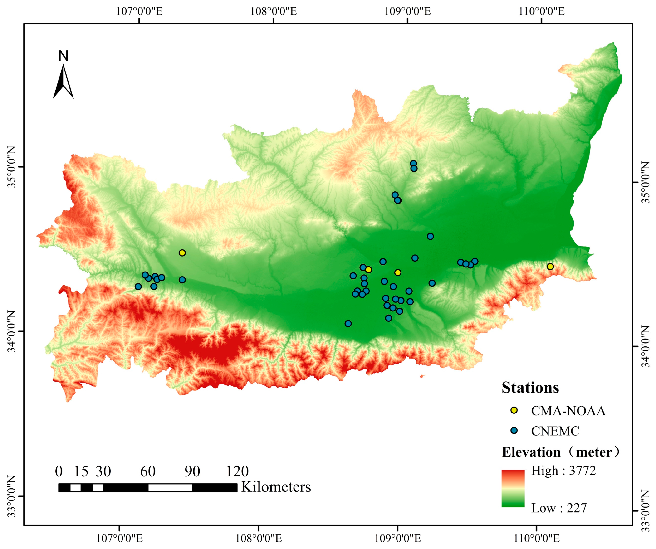
The Guanzhong Region, showed in Figure 1, situated in the central part of Shaanxi Province, China, which spans approximately 106°56′~110°22′ E longitude and 33°39′~35°52′ N latitude, has been selected as the research area because of its typical plain topography and because it is one of the most severely polluted air regions, with representative cities such as Xi’an, Xianyang, and Weinan consistently ranking among the bottom 20 of 168 key cities of China. Bounded by the Qinling Mountains to the south and the Loess Plateau to the north, it stretches about 360 km from east to west and has an average elevation of around 500 m. The terrain gradually descends from west to east. The region exhibits a warm temperate continental monsoon climate, characterized by an average annual temperature of 12 °C to 14 °C and an annual average rainfall of 530 to 750 mm. Dominant prevailing winds throughout the year are from the northeast, followed by secondary winds from the southwest. The average relative humidity ranges between 60% and 70%. Encompassing five cities—Xi’an, Baoji, Xianyang, Weinan, and Tongchuan—the Guanzhong Region spans a total area of 55,623 square kilometers and is classified as one of China’s four major geographical divisions, the northern region.

Figure 1.
Distribution of CMA-NOAA and CNEMC monitoring stations in the research area.
2.2. Data Sources
A substantial volume of high-quality data stands as a prerequisite for effective machine-learning applications. As illustrated in Table 1, the data utilized in this research comprised station data published by the China National Environmental Monitoring Center (CNEMC) and satellite imagery data from the Google Earth Engine (GEE, https://earthengine.google.com, accessed on 16 July 2023) platform and the United States Geological Survey (USGS, https://earthexplorer.usgs.gov/, accessed on 16 July 2023) including MODIS AOD/SR, Landsat 8 OLI, and Sentinel-2, as well as meteorological data from ground-based monitoring stations operated by the China Meteorological Administration (CMA) and the National Oceanic and Atmospheric Administration (NOAA) in the United States. All of these datasets are openly accessible.

Table 1.
Description of the data employed in the research.
2.2.1. MODIS Data
The moderate-resolution imaging spectroradiometer (MODIS) is equipped on both the Terra and Aqua satellites. It captures data in 36 spectral bands covering the spectral range from 0.4 μm (visible light) to 14.4 μm (thermal infrared) with spatial resolutions ranging from 250 to 1000 m. These instruments provide complete spectral coverage and revisit the Chinese mainland area 1–2 times per day [22]. This research utilized the daily land aerosol optical depth (AOD) data MCD19A2 and daily surface reflectance (SR) data MOD09GA.
2.2.2. Landsat 8 Data
The Landsat 8 satellite was launched in February 2013 and began offering free data in May of the same year. It carries two sensors: the operational land imager (OLI) and the thermal infrared sensor (TIRS) [23]. The OLI sensor comprises 9 spectral bands, with a spatial resolution of 15 m for panchromatic bands and 30 m for other bands. The imaging swath width is 185 × 185 km, with a revisit cycle of 16 days. In this research, we utilized band data from Landsat 8 Collection 2 Tier 1 Raw Scenes products.
2.2.3. Sentinel-2 Data
Sentinel-2 is an Earth observation mission from the Copernicus program by the European Space Agency, primarily aimed at observing the Earth’s surface to provide various remote-sensing services such as agricultural monitoring, emergencies management, land-cover classification, or water quality. This mission consists of two identical satellites, Sentinel-2A and Sentinel-2B, equipped with 13 spectral bands ranging from the visible to the shortwave infrared spectrum. The spatial resolutions are 10 m, 20 m, and 60 m, respectively. The revisit period for each satellite is 10 days [24]. In this research, we utilized surface reflectance data from Sentinel-2A.
2.2.4. Air Quality Data
The China National Environmental Monitoring Center (CNEMC) is a specialized institution under the Ministry of Ecology and Environment. It is responsible for nationwide environmental monitoring across various domains, including air, water, ecology, soil, coastal areas, noise, and pollution sources. Presently, CNEMC provides real-time monitoring concentration data for PM2.5, PM10, O3, CO, NO2, and SO2. These datasets serve as the primary foundation for estimating surface air pollutant concentrations based on remote sensing and can be collected from the CNEMC platform (http://www.cnemc.cn, accessed on 16 July 2023). CNEMC operates over 1500 monitoring stations throughout mainland China, including 41 stations in the research area (Figure 1).
2.2.5. Meteorological Data
The National Oceanic and Atmospheric Administration (NOAA) is the governing body responsible for meteorological operations in the United States. In 2013, the China Meteorological Administration (CMA) and NOAA entered into a collaborative agreement, authorizing NOAA to publicly release meteorological data for mainland China on the Internet (https://gis.ncdc.noaa.gov/maps/ncei/cdo/hourly, accessed on 16 July 2023). These data are updated every three hours. This research utilized atmospheric factors including atmospheric pressure (PRS), relative humidity (RH), temperature (T), wind direction (WD), and wind speed (WS) [25]. Particularly, the calculation of relative humidity was obtained using the following formula [26]:
where T and dew point temperature (Td) are in Celsius, RH is in percent, ln represents the natural logarithm, the constant a is 17.27, and the constant b is 237.7 °C.
CMA-NOAA has more than 300 cooperative monitoring stations in mainland China, including four stations in the research area (Figure 1).
2.3. Data Preprocessing
Due to the wide variety of data sources utilized in this research, significant differences exist in data types and resolutions. Therefore, preprocessing and spatiotemporal matching of the aforementioned research data are imperative.
(1) Regarding outliers in land stations, we referenced the “Technical Regulation on Ambient Air Quality Index (on trial)” and conducted outlier removal procedures accordingly. Quality control tools provided by Google Earth Engine (GEE) were employed to eliminate satellite data samples significantly affected by clouds. With the MODIS data, MCD19A2 removed clouds based on the AOD_QA quality control band (Bits8-11 = “0000”), while MOD09GA removed clouds based on the state_1 km band (Bits0-2 = “000” and Bit10 = “0”). Landsat 8 data removed clouds based on the QA_PIXEL quality control band (Bits3-4 = 00), and Sentinel-2 data used the QA60 band for quality control, retaining data with QA60 = 0 [27]. High-quality satellite remote-sensing images of the research area were obtained through mosaicking, projection transformation, resampling, reprojection, and cropping. Kriging interpolation was applied to meteorological station data to acquire spatial meteorological data in the research area.
(2) The above data require spatial and temporal matching due to differences in observation time, temporal resolution and spatial resolution. Regarding the different temporal resolutions of the data, the imaging time properties of each satellite are the time reference for time matching. The imaging time properties of each satellite are regarded as the temporal reference to match air quality data and meteorological data. For MODIS satellite products that provide daily averaged data, the air quality and meteorological data are processed into daily averages and matched accordingly. For Landsat 8 and Sentinel-2 satellite products that provide instantaneous data, the air quality and meteorological data are matched using linear interpolation and a time buffer interval of ±1 h. The near analysis algorithm (NAA) has been employed for spatial matching to integrate the CEMC observations and NOAA datasets. As for the normalized difference vegetation index (NDVI), it was calculated by the NIR and red bands according to Formula (3) in MODIS SR, Landsat 8 OLI, and Sentinel-2, while it was matched by the NDVI band of MOD13A2 product in MODIS AOD.
(3) Given the differences in data scales and measurement units, normalization of the data is necessary to minimize model errors. This research employed the min–max normalization method:
where I represents the original feature data, and represent the minimum and maximum values of the feature data, respectively, and represents the normalized feature data.
2.4. Methods
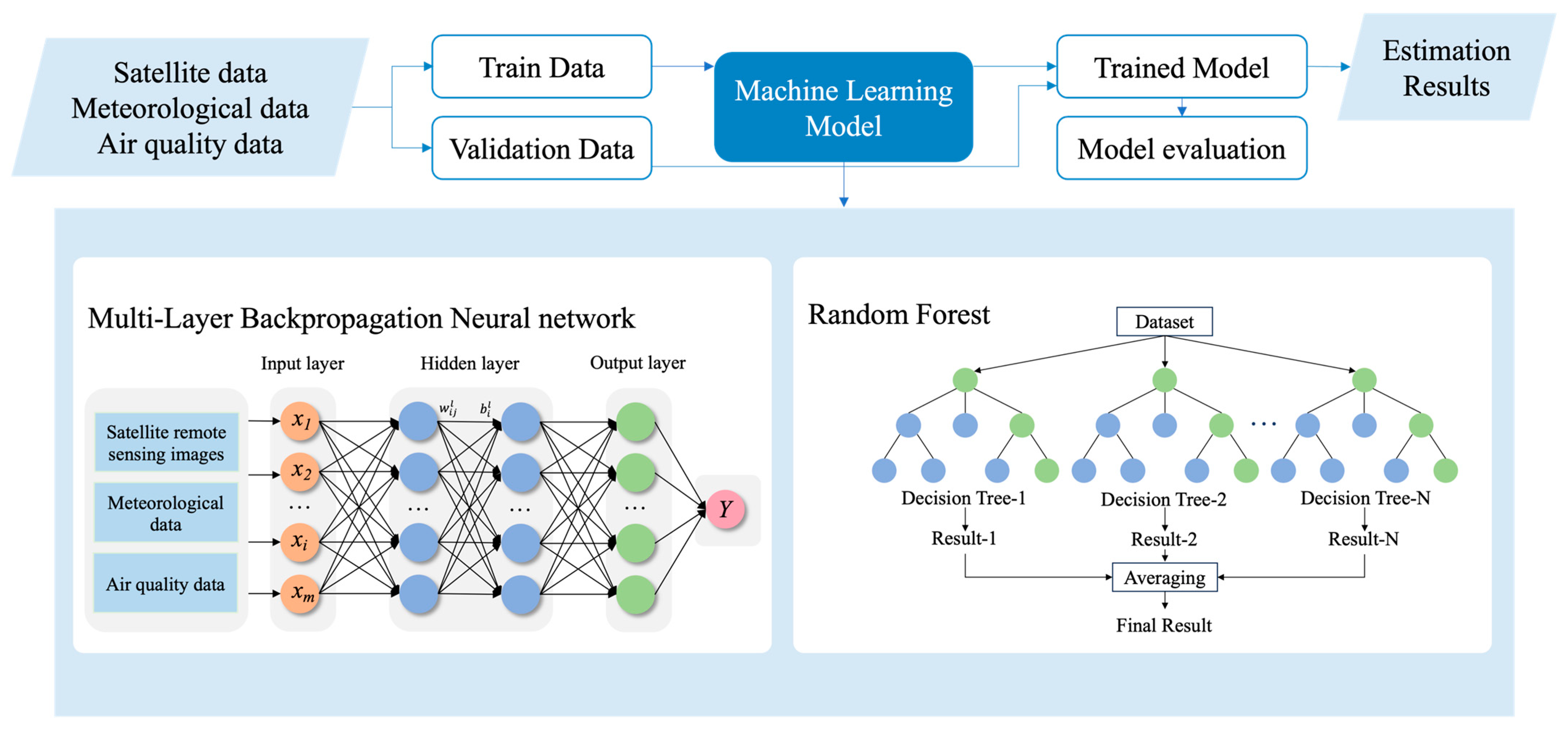
As shown in Figure 2, machine-learning methods were employed to explore and establish the relationships between internal features to achieve spatial estimation after completing the data collection and preprocessing. This research employed multi-layer backpropagation neural network (MLBPN) and random forest (RF) models, which have demonstrated a favorable performance in air pollutant estimation, as evidenced by both this experiment and previous literature. In order to strike a balance between training the model effectively and thoroughly evaluating its performance, the dataset was partitioned into training and testing sets using an 80/20 split [28]. Furthermore, given the temporal properties of data and the large data volume, cross-validation was performed using the “Hold-out Method”. All the experiments were conducted on a Windows 11 Professional 64-bit operating system with 12th Gen Intel(R) Core(TM)i7-12700KF CPU configuration and NVIDIA GeForce RTX 3070Ti GPU configuration.
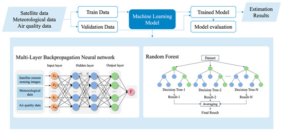
Figure 2.
Diagram of the research strategy.
2.4.1. Multi-Layer Backpropagation Neural Network (MLBPN)
The multi-layer backpropagation neural network (MLBPN) model is a type of multi-layer feedforward neural network trained using the backpropagation algorithm, which demonstrates clear advantages in addressing nonlinear system problems. The MLBPN-based model consists of an input layer, several hidden layers, and an output layer [29]. Upon providing a set of learning samples to the MLBPN-based model, activation values propagate from the input layer through the intermediate hidden layers to the output layer, acquiring the network’s input response at the output layer neurons. Subsequently, the connection weight values are incrementally adjusted layer by layer, from the output layer through each intermediate layer, following the direction to minimize the target output and actual error, ultimately returning to the input layer. In Figure 2, xi represents the input value of this neural network (i = 1, 2, …, m), and Y represents the output value. represents the connection weight between node j in hidden layer l-1 and node i in hidden layer l. represents the bias of node i in layer l. The transfer between different hidden layers utilizes the Tansig function equation, while the Purelin function equation is employed between the hidden layer and the output layer [30,31,32]. They are expressed as follows:
The optimal number of nodes for the hidden layers in the model is set to [15,15]. The Levenberg–Marquardt (LM) algorithm is utilized for neural network training using the trainlm function, with the maximum training epochs set to 500, the network training goal set to 0.001, and a learning rate of 0.1.
2.4.2. Random Forest (RF)
The random forest (RF) algorithm is an optimization of the decision tree method, constructing multiple independent decision trees and averaging their outcomes for fitting. This approach effectively addresses the issues of low accuracy and overfitting commonly associated with individual decision trees, thereby enhancing the generalization ability of the algorithm. The decision trees in a random forest are binary trees, following the recursive top-down splitting pattern, and nodes are split based on the principle of minimizing node impurity. In this research, the TreeBagger function from the Matlab R2021b software was employed for remote-sensing estimation of surface air pollutant concentrations. During the model optimization phase, adjustments were made to enhance the estimation accuracy by setting the number of decision trees to 100 and the minimum leaf size to 5.
2.5. Validation
In order to better evaluate the model, four statistical indicators, the coefficient of determination (R2), root mean square error (RMSE), mean absolute error (MAE), and mean error (ME), were chosen for comparative analysis in this research [33]. Their calculation formulas are as follows, respectively:
where denotes the pollutant concentration estimation value, denotes the pollutant concentration measured value, and denotes the number of samples.
3. Results
3.1. Model Performance
The comparison of the estimation performances of the RF and MLBPN models for the concentrations of air pollutants, based on the MODIS AOD data with a total of 15,577 samples in the research area from 2019 to 2022, is shown in Table 2. Compared to the MLBPN-based model, the R2 of the RF-based model improves by about 0.1 for PM2.5, O3, and CO and 0.2 for PM10, NO2, and SO2; at the same time, the RMSE and the MAE are significantly decreased. These values indicate that the RF-based model has a better estimation performance than the MLBPN-based model. In the context of the RF-based model, the R2 values for PM2.5, PM10, and O3 are around 0.9; for NO2 and CO exceed 0.7; and for SO2 surpass 0.5, which indicates that the MODIS AOD data can accurately estimate the continuous spatial distribution of air pollutants.
Table 2.
Estimation performances of the RF and MLBPN models using MODIS AOD data.
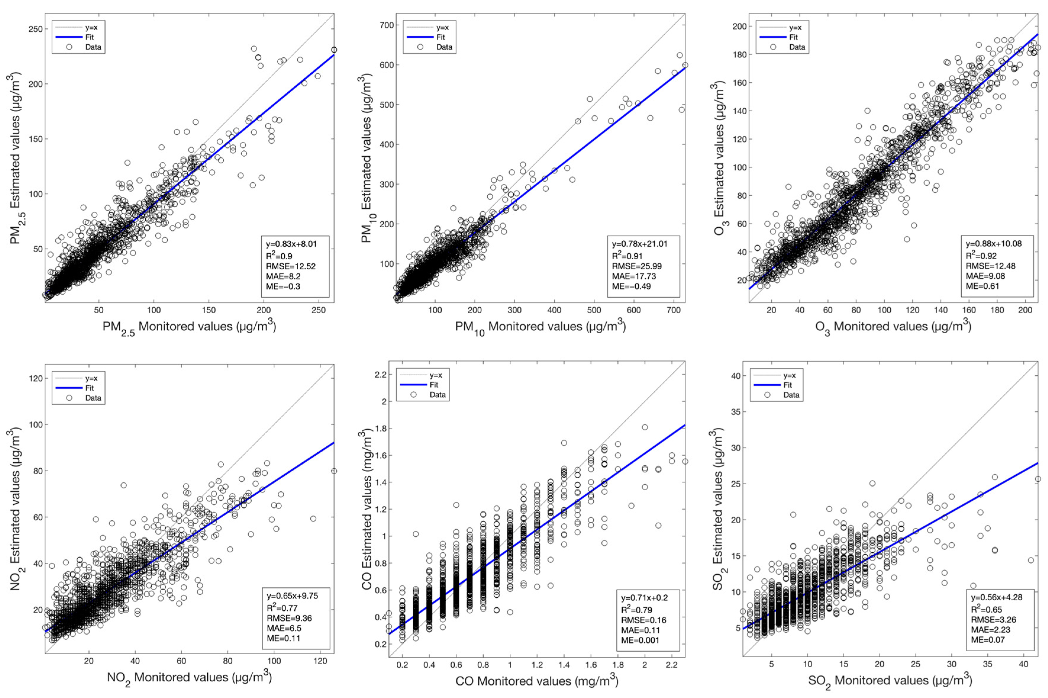
The comparison of the estimation performances of RF and MLBPN models for the concentrations of air pollutants, based on the MODIS SR data with a total of 7821 samples in the research area from 2019 to 2022, is shown in Table 3. Compared to the MLBPN-based model, the R2 values of the RF-based model for PM2.5, PM10, O3, NO2, and CO improve by about 0.1; simultaneously, the RMSE and the MAE are significantly decreased. These values indicate that the RF-based model has a better estimation performance than the MLBPN-based model. For the RF-based model, the R2 values for PM2.5 and O3 are around 0.8; PM10 exceeds 0.7; NO2 and CO are around 0.6; and SO2 surpasses 0.3. These results indicate that the MODIS SR data can effectively estimate the continuous spatial distribution of PM2.5, PM10, O3, NO2, and CO.
Table 3.
Estimation performances of the RF and MLBPN models using MODIS SR data.
The comparison of the estimation performances of the RF and MLBPN models for the concentrations of air pollutants, based on the Landsat 8 OLI data with a total of 1181 samples in the research area from 2019 to 2022, is shown in Table 4. It can be seen that the difference in accuracy between these two models is relatively close, but on the whole, the MLBPN-based model performs better than the RF-based model. For the MLBPN-based model, the R2 of PM2.5 and O3 is close to 0.9; that of PM10 and CO is close to 0.8; and that of NO2 and SO2 is around 0.6, which indicates that the Landsat 8 OLI data can accurately estimate the continuous spatial distribution of air pollutants.
Table 4.
Estimation performances of the RF and MLBPN models using Landsat 8 OLI data.
The comparison of the estimation performances of RF and MLBPN models for the concentrations of air pollutants, based on the Sentinel-2 data with a total of 7933 samples in the research area from 2019 to 2022, is shown in Table 5. Compared to the MLBPN-based model, the R2 of the RF-based model improves about 0.1 for O3, 0.15 for PM2.5 and PM10, 0.2 for NO2 and CO, and 0.25 for SO2; at the same time, the RMSE and the MAE are significantly decreased. These values indicate that the RF-based model has a better estimation performance than the MLBPN-based model. The RF-based model demonstrates a strong performance with R2 values exceeding 0.9 for PM2.5, PM10, and O3; close to 0.8 for NO2 and CO; and larger than 0.6 for SO2, which indicates that the Sentinel-2 data can accurately estimate the continuous spatial distribution of air pollutants.
Table 5.
Estimation performances of the RF and MLBPN models using Sentinel-2 data.
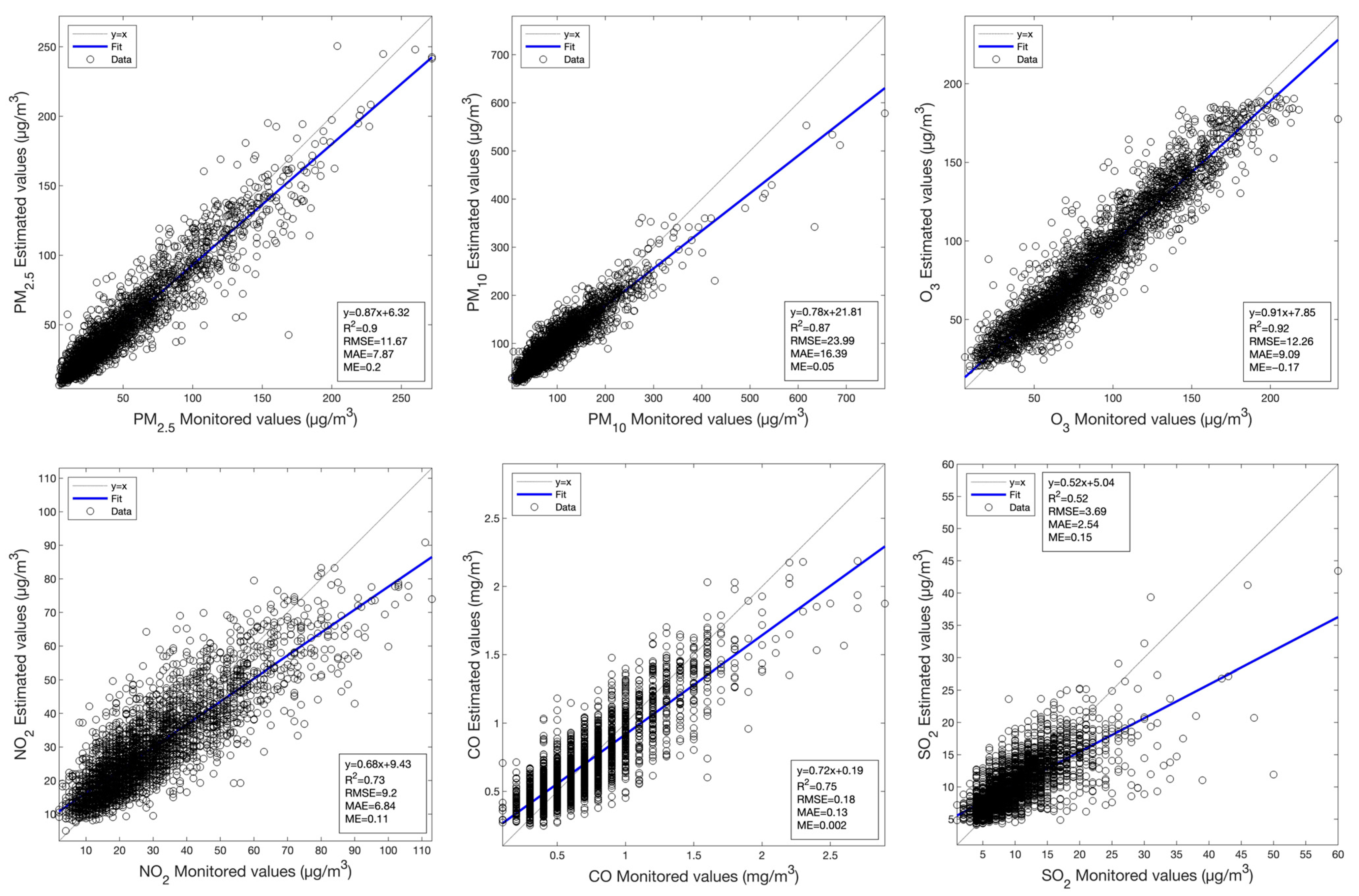
In summary, the RF-based model has revealed a better estimation performance using the satellite imagery from MODIS AOD/SR and Sentinel-2, and for the MLBPN-based model, a better estimation performance can be obtained from the use of Landsat 8 OLI. Scatterplots between the monitored values and the values estimated by the RF-based model using MODIS AOD data for air pollutants are presented in Figure 3. Similar scatterplots between the monitored values and the values estimated by the corresponding optimal model using MODIS SR, Landsat 8 OLI, and Sentinel-2 data are provided in Figure A1, Figure A2 and Figure A3 in Appendix A.
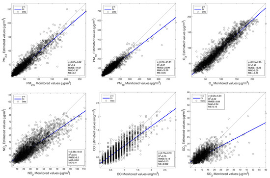
Figure 3.
Scatterplots between the monitored values and the values estimated by the RF model using MODIS AOD data for the various primary air pollutants.
3.2. Spatiotemporal Analysis
Although the RF-based model with Sentinel-2 revealed a slightly better performance for the estimation of PM10, NO2, CO, and SO2 than that with MODIS AOD, such differences are not significant. Combined with the consideration that the MODIS satellite has a high temporal resolution, covering the entire research area and revealing a better performance for the PM2.5 and O3 estimations, the MODIS AOD data have been confirmed as the basic satellite data for spatiotemporal analysis in the research area.
3.2.1. Temporal Distribution Characteristics
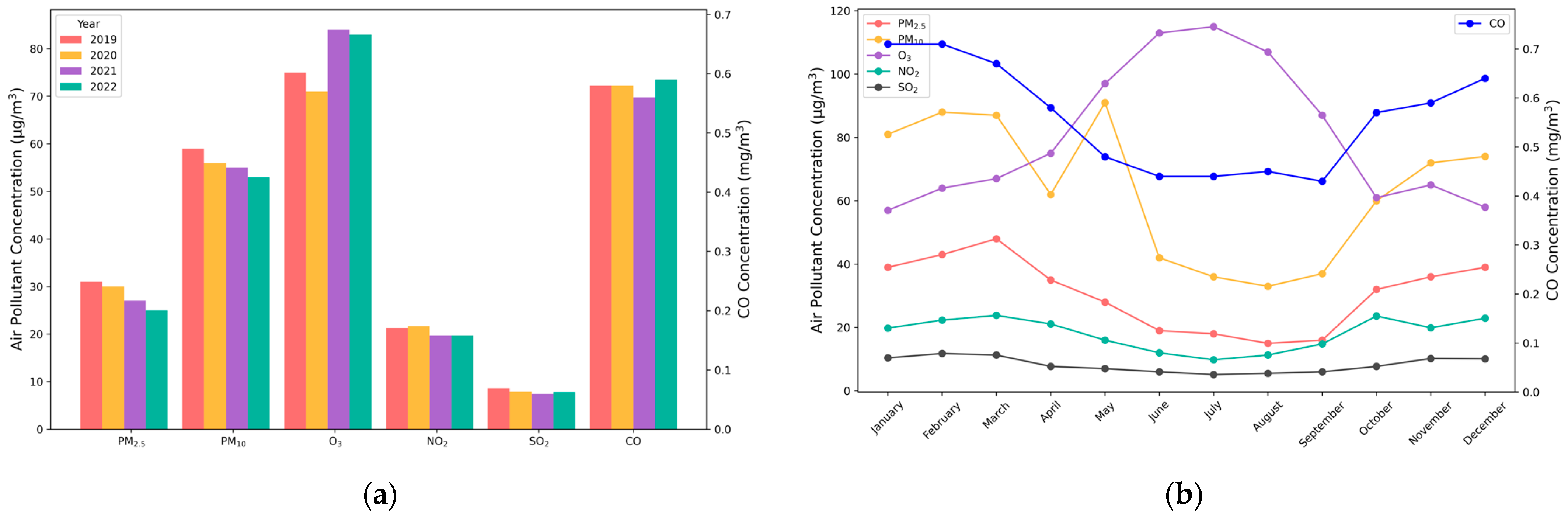
The annual average concentrations of air pollutants in the research area from 2019 to 2022 display various trends in Figure 4a: PM2.5, PM10, NO2, and SO2 display a consistent decrease, whereas O3 and CO display a trend of decreasing followed by increasing. The annual average concentrations of PM2.5 and PM10 decreased by approximately 6 μg/m3, with a decrease of 19% and 10%, respectively. The decreases in NO2 and SO2 were 8% and 10%, respectively. CO concentration decreased by 0.02 mg/m3 in 2021, followed by an increase of 0.03 mg/m3 in 2022. However, the annual concentration of CO was relatively stable and remained below 0.6 mg/m3. O3 concentration decreased by 3.4 μg/m3 in 2020, followed by an increase of 12.4 μg/m3 in 2021, with an overall increase of 11%, and finally remained around 83 μg/m3.

Figure 4.
Temporal change trends of different air pollutants in the research area: (a) Annual average values from 2019 to 2022; (b) Monthly average values in 2021.
The monthly concentrations of air pollutants in the research area in 2021 are shown in Figure 4b. PM2.5, PM10, NO2, CO, and SO2 concentrations show a “U”-shaped monthly trend, with the lowest pollutant concentrations in summer and the highest in winter. The reasons are analyzed: the increase in pollutant concentrations is primarily attributed to the heating season from November to March, involving substantial burning of coal, biomass, and biofuels, and an inverse temperature and high atmospheric pressure, causing pollutants to accumulate in the lower atmosphere with the movement of the descending airflow. On the contrary, the decrease in pollutant concentrations is primarily attributed to lower atmospheric pressure and higher temperatures from May to September, creating atmospheric instability and favoring pollutant dispersion, and increased rainfall during this period contributes to air purification. Notably, PM10 exhibited a high concentration anomaly in May, attributed to frequent sandstorms caused by cold air and strong winds, increasing dust and particulate matter levels, and worsening pollution.
O3 concentration shows the opposite trend to the other pollutants, peaking in summer, followed by spring, autumn, and winter. This is because near-surface O3 primarily arises from precursor elements such as volatile organic compounds (VOCs), carbon monoxide (CO), and nitrogen oxides (NOx) through complex photochemical reactions heavily influenced by sunlight and radiation intensity.
3.2.2. Spatial Distribution Characteristics
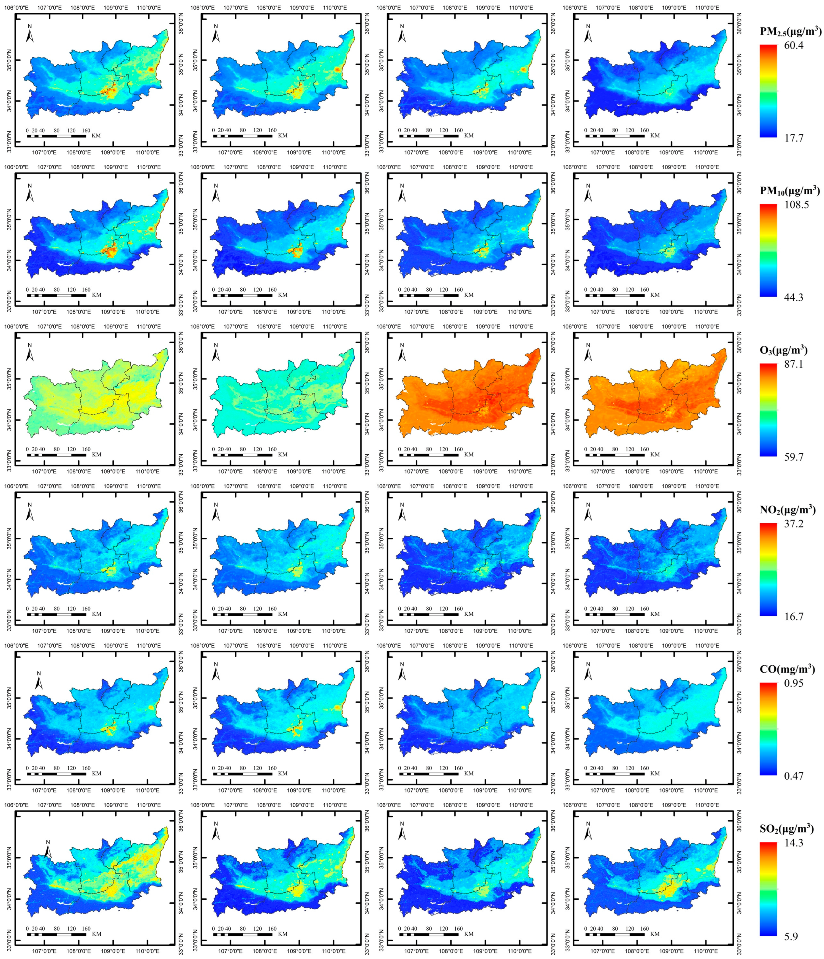
The annual-scale spatial distribution maps of air pollutants in the research area from 2019 to 2022, estimated by MODIS AOD data, showcase a consistent trend: a gradual increase from west to east, with the distribution of higher concentrations in the center of the built-up areas and lower in the surrounding rural areas (as depicted in Figure 5).
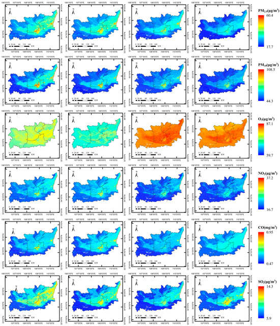
Figure 5.
Spatial distribution of the annual average values of different air pollutants from 2019 to 2022.
The high-pollution areas are mainly concentrated in the Guanzhong urban agglomeration, especially in the southern part of Xianyang, the northern part of Xi’an, the entire Weinan region, the central part of Baoji, and parts of southern Tongchuan. These areas are located in the lower elevation basin, bordered by the Loess Plateau in the north and the Qinling Mountains in the south, forming a trumpet-shaped topography with a higher west and lower east. East and northeast winds prevail in Guanzhong all year round, and the airflow enters from the eastern entrance along the Weihe Plain, making the concentration of air pollutants higher in the low-altitude areas within the basin. The low-pollution areas are mainly in the surrounding rural areas, with high-altitude mountain ranges, high vegetation cover, low human activities, and low industrial pollution.
Notably, PM2.5, PM10, NO2, CO, and SO2 show the highest concentration distribution in the urban areas of Xi’an and the adjoining regions bordering Shanxi Province and Weinan City, while O3 shows the lowest concentration distribution. This is because the meteorological conditions for the formation of O3 pollution are low humidity, low pressure, high temperature, and low wind, which is the opposite to the correlation between the other pollutants and meteorological factors.
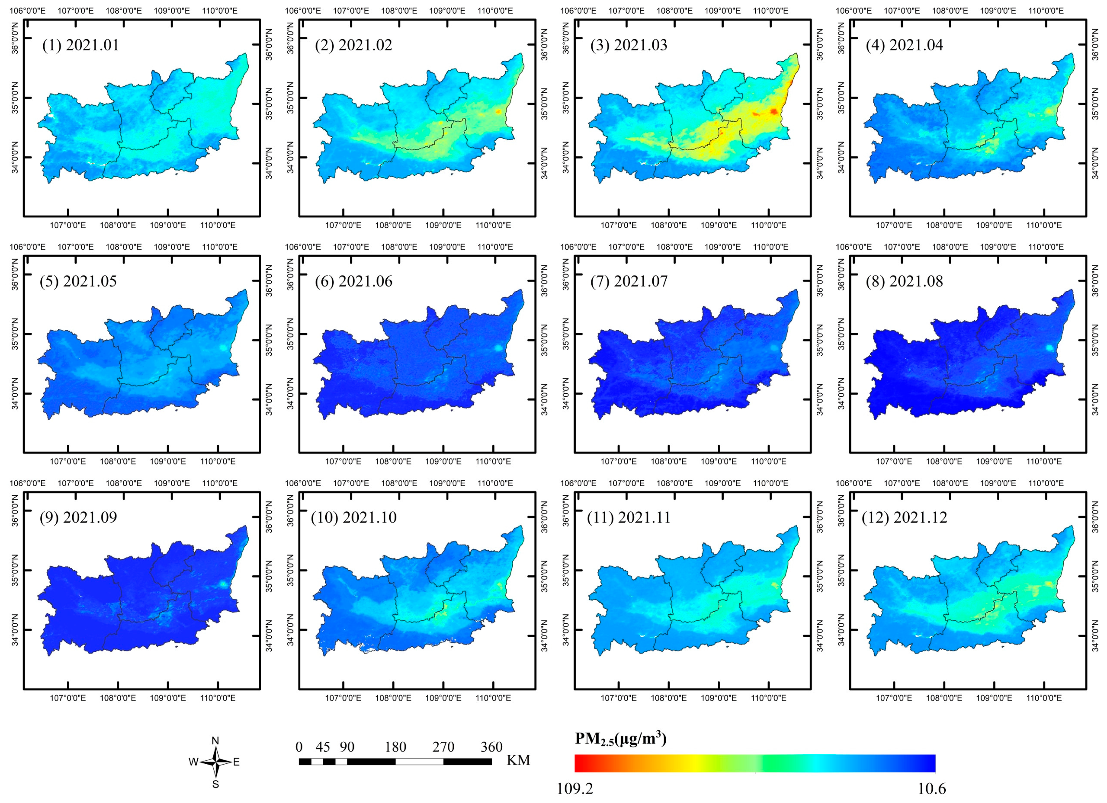
Figure 6 illustrates the spatial distribution of the monthly average concentration of PM2.5 in the research area in 2021. The spatial distribution of monthly average concentrations of other air pollutants can be found in Figure A4, Figure A5, Figure A6, Figure A7 and Figure A8 in Appendix B. It can be found that the monthly spatial distribution of PM2.5, PM10, NO2, CO, and SO2 is consistent with the annual spatial distribution. Meanwhile, pollutant concentrations are low from May to September and high in other months. The spatial distribution of O3 shows distinct fluctuations: concentrations are high in the center area and low in the peripheral area from March to October, whereas this pattern is reversed in other months. This variation reflects the complexity of O3 pollution with seasonal and meteorological conditions.
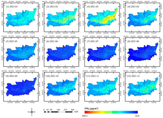
Figure 6.
Spatial distribution of the monthly average PM2.5 concentrations in 2021.
4. Discussion
In this research, RF- and MLBPN-based models have been respectively proposed for the estimation of the ground surface concentrations of PM2.5, PM10, O3, NO2, CO, and SO2 from the various satellite imagery of MODIS AOD, MODIS SR, Landsat 8 OLI, and Sentinel-2. The conducted experiments demonstrate that (a) except for the Landsat 8 OLI data, the RF-based model revealed a better estimation performance than the MLBPN-based model using the satellite imagery from MODIS AOD/SR and Sentinel-2; (b) the results estimated from the MODIS AOD, Sentinel-2, and Landsat 8 OLI satellite data revealed significantly higher accuracies than MODIS SR data; (c) the RF-based model combined with the MODIS AOD data revealed the best performance for the estimation of PM2.5 and O3—the R2 and RMSE reached 0.90 and 11.67 μg/m3 for PM2.5, and 0.92 and 12.26 μg/m3 for O3, respectively; while the RF-based model combined with the Sentinel-2 or MODIS AOD data achieved a comparable performance for PM10, NO2, CO, and SO2—the R2 and RMSE reached ca. 0.90 and 25 μg/m3 for PM10, ca. 0.75 and 9.3 μg/m3 for NO2, ca. 0.77 and 170 mg/m3 for CO, and ca. 0.6 and 3.5 μg/m3 for SO2, respectively.
Considering the estimation performance and the temporal resolution of the satellite data, the RF-based model together with the MODIS AOD data can be treated as the optimal combination of “model and data”—for PM2.5, PM10, and O3, the estimation results with the R2 of ca. 0.9 are convincing; for NO2 and CO, the results with the R2 close to 0.8 are still reliable; while for the SO2, the R2 reaches 0.65, and hence the estimation results can only be used under some kinds of specific conditions. The estimation accuracy of trace gases, especially SO2, is relatively lower than that of particulate matter. This may be due to the fact that the spectra range of the satellites used in the research did not include the ultraviolet (UV) band, which is crucial for the estimation of some trace gases, especially SO2.
Based on the discussions mentioned above, the RF-based model with the MODIS AOD data was employed for the analysis of the spatiotemporal distributions in the Guanzhong Region, China. In terms of annual scale changes, the average concentrations of PM2.5, PM10, NO2, and SO2 show a decreasing trend, while CO remains relatively stable, and O3 shows an increasing trend from 2019 to 2022. In terms of monthly scale changes, the concentrations of PM2.5, PM10, NO2, CO, and SO2 in 2021 showed a “U”-shaped trend, with the lowest pollutant concentrations in the summer and the highest in the winter, and the O3 concentration showed the opposite trend. The spatial distribution of air pollution presents a gradual increase from west to east in the research area, with the distribution of higher concentrations in the center of the built-up areas and lower in the surrounding rural areas.
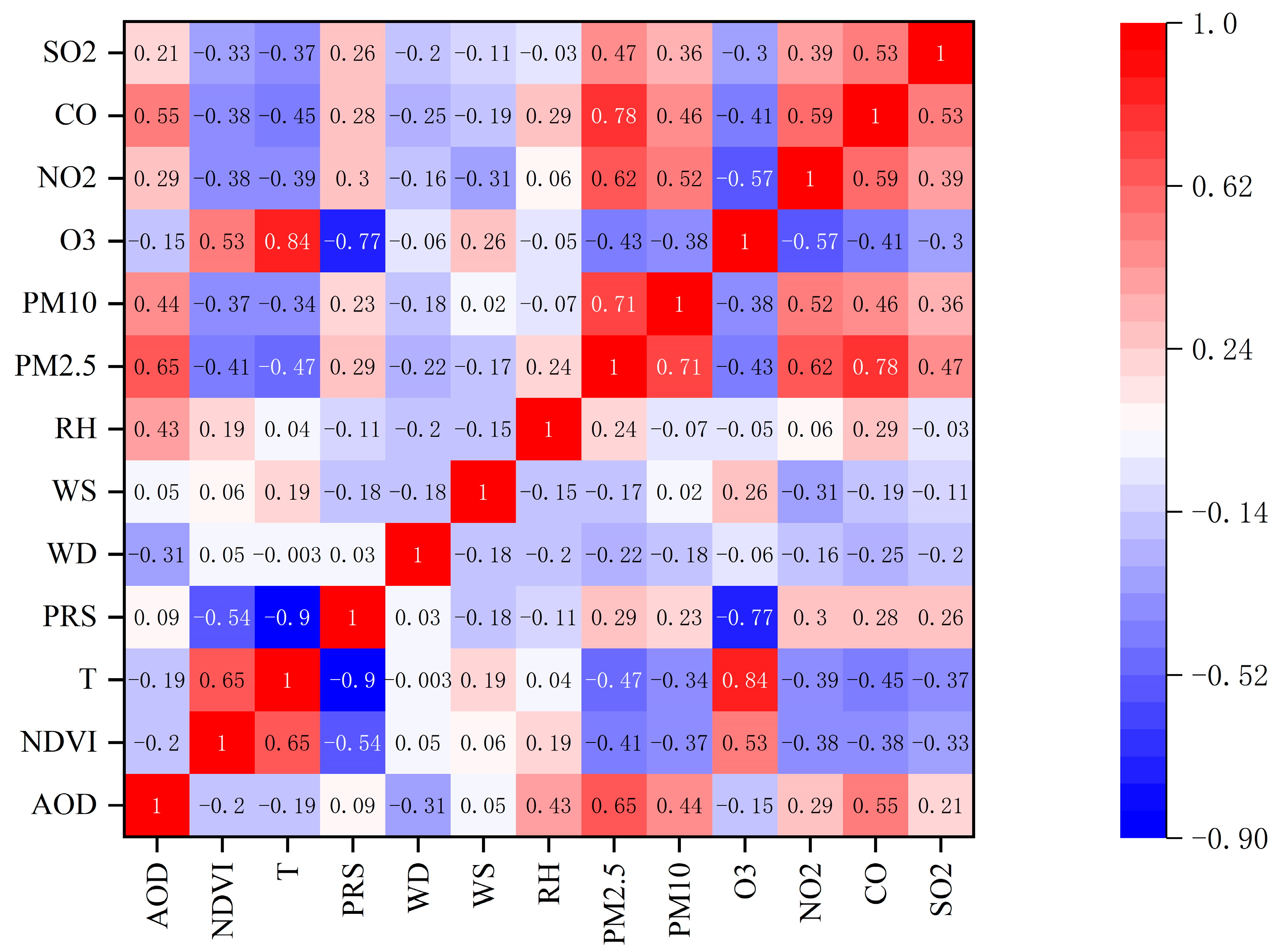
One particular aspect of the research is that we have also added meteorological data in addition to satellite remote-sensing data. The Pearson correlation coefficient heatmap based on MODIS AOD data, as shown in Figure 7, demonstrates a strong correlation between meteorological data and air pollutant concentrations.
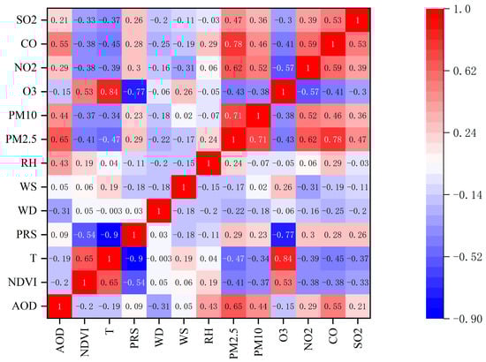
Figure 7.
Pearson correlation coefficient of modelling parameters based on MODIS AOD data.
Additionally, Table 6 presents the results of a comparative experiment conducted using meteorological parameters as independent variables based on the RF model and MODIS AOD data. It indicates a significant improvement in model accuracy when meteorological data are included, with the R2 increasing by approximately 0.3 for PM2.5 and CO, and approximately 0.4 for PM10, O3, NO2, and SO2.
Table 6.
Estimation performances with meteorological parameters as independent variables based on the RF model and MODIS AOD data.
However, the publicly available meteorological data from the National Oceanic and Atmospheric Administration consisted of only four stations within the research area. The limited meteorological data could have affected the generic nature of the sample data for model training and thereby could reduce the estimation accuracy and reliability in some kinds of specific situations. Hence, non-public meteorological data should be considered in further studies for a more detailed and accurate estimation of air pollutant concentrations.
5. Conclusions
This research compared the estimation results generated by different models from diverse types of satellite data, and the “optimal” model and satellite data were identified to provide one practical method for air pollutant concentration estimation. Furthermore, an analysis of spatiotemporal variations in the various primary air pollutants was conducted, which proved that the air quality tends to be better in mountainous areas than in urban centers, highlighting significant implications for public health. This discovery suggests that individuals may engage in more outdoor activities in mountainous regions to enhance opportunities for aerobic exercise, thereby promoting both physical and mental well-being. Additionally, it indicates that the air quality in the summer tends to be better than the other three seasons, suggesting the possibility of relaxing certain environmental restrictive policies, such as the bans on burning straw during this season.
To sum up, the conducted research can provide decision support for the development of relevant environmental protection measures to improve the air environmental quality and foster socioeconomic development in the Guanzhong Region.
Author Contributions
Y.L. and M.Z. conceived and designed the study; Y.L., M.Z., G.M., H.R. and E.Y. collected the data and completed the experiments; M.Z. initiated the overall research question and found funding for this project; Y.L. drafted the paper; M.Z. critically read and revised the draft. All authors have read and agreed to the published version of the manuscript.
Funding
This work was funded in part by the Key Research and Development Program of Shaanxi Province (China) under Grant 2020SF-434, and in part by the National Natural Science Foundation of China under Grant 41871315.
Institutional Review Board Statement
Not applicable.
Informed Consent Statement
Not applicable.
Data Availability Statement
All the data used in this study are publicly available, which can be found at https://earthengine.google.com, https://earthexplorer.usgs.gov/, http://www.cnemc.cn and https://gis.ncdc.noaa.gov/maps/ncei/cdo/hourly (accessed on 16 July 2023).
Acknowledgments
This research was supported by the Strategic Priority Research Program of the Chinese Academy of Sciences under Grant XDB40020200, and the Key Research and Development Program of Shaanxi Province (China) under Grants 2021SF-498 and 2021SF-501.
Conflicts of Interest
The authors declare no conflicts of interest.
Appendix A. Scatterplots between the Monitored Values and the Estimated Values
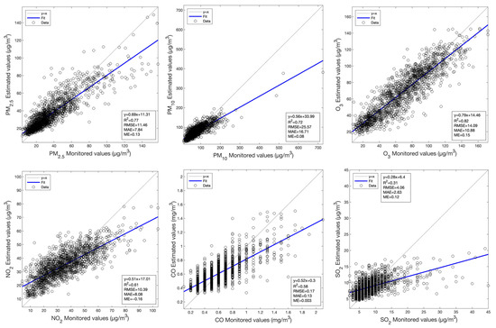
Figure A1.
Scatterplots between the monitored values and the values estimated by the RF model using MODIS SR data for the various primary air pollutants.
Figure A1.
Scatterplots between the monitored values and the values estimated by the RF model using MODIS SR data for the various primary air pollutants.
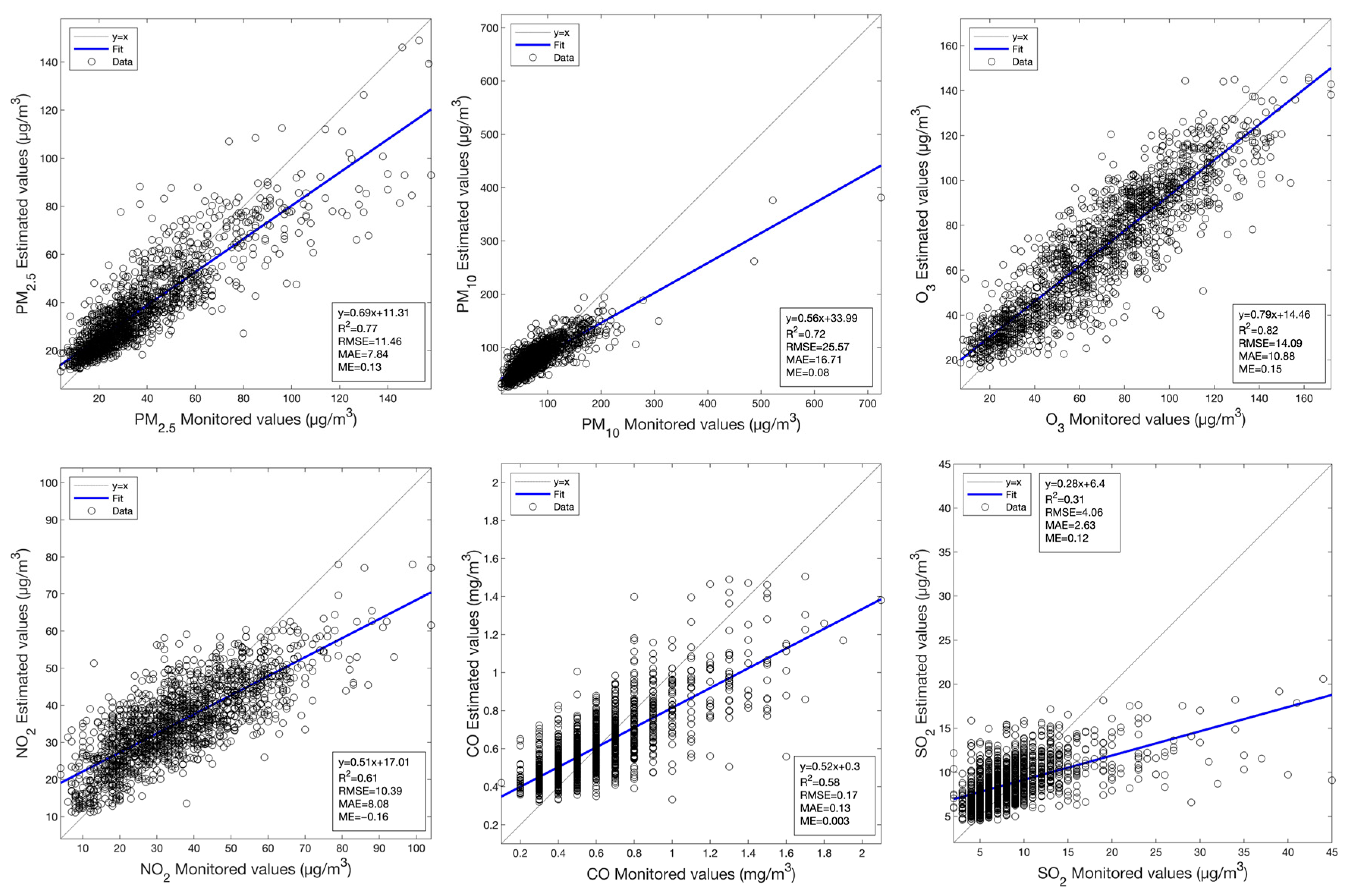
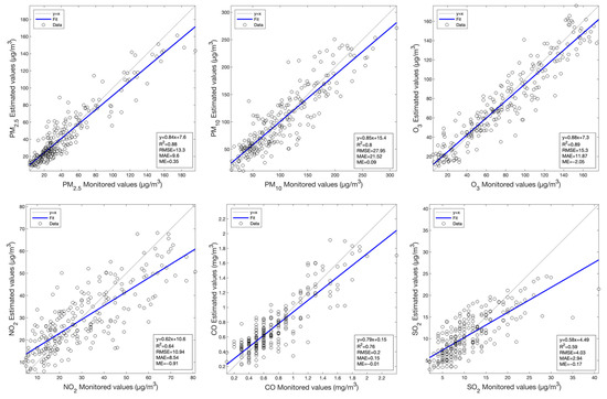
Figure A2.
Scatterplots between the monitored values and the values estimated by the MLBPN model using Landsat 8 OLI data for the various primary air pollutants.
Figure A2.
Scatterplots between the monitored values and the values estimated by the MLBPN model using Landsat 8 OLI data for the various primary air pollutants.
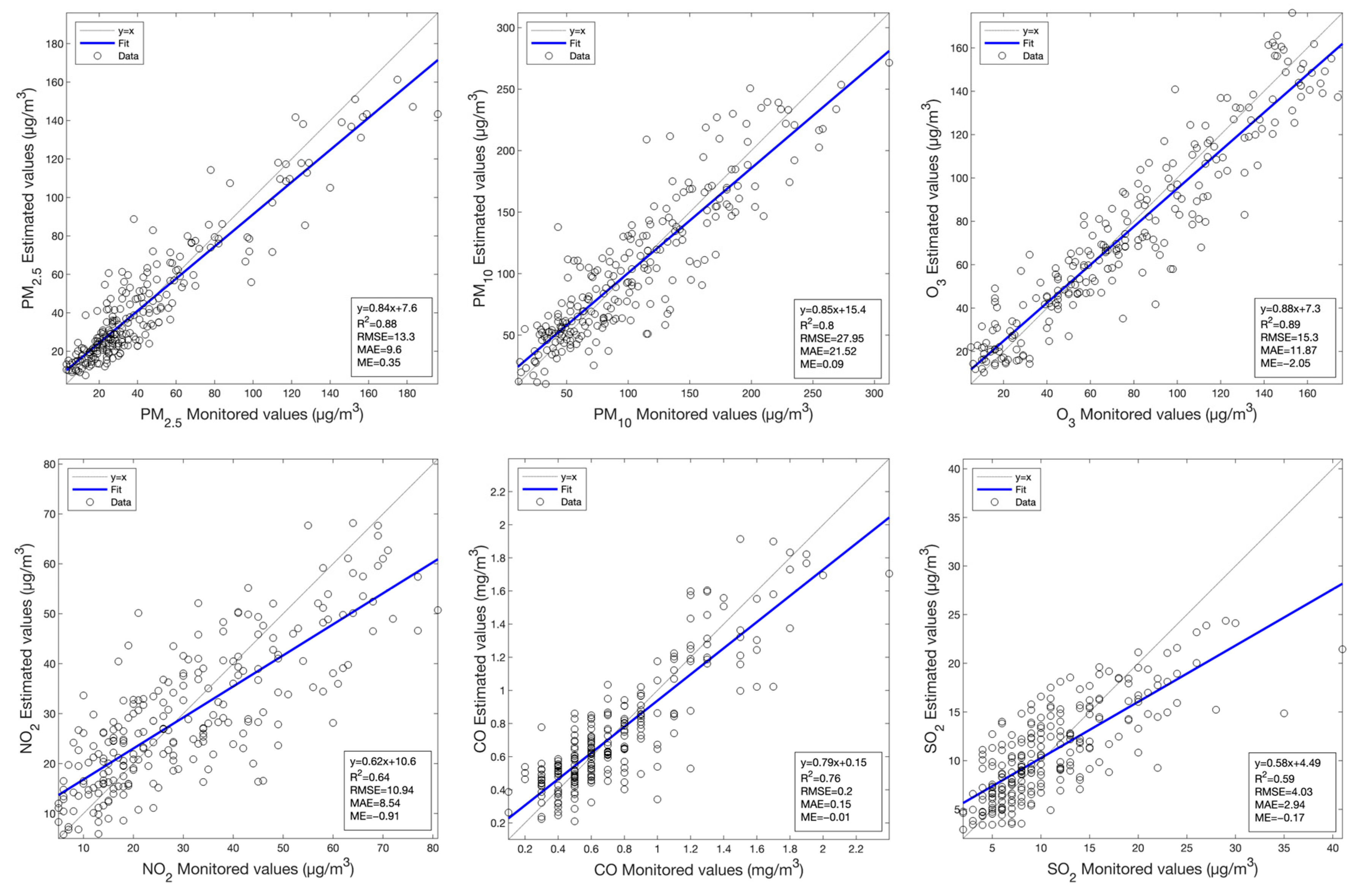
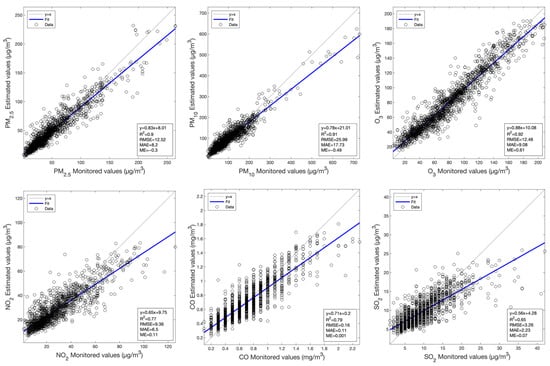
Figure A3.
Scatterplots between the monitored values and the values estimated by the RF model using Sentinel-2 data for the various primary air pollutants.
Figure A3.
Scatterplots between the monitored values and the values estimated by the RF model using Sentinel-2 data for the various primary air pollutants.
Appendix B. Spatial Distribution of the Monthly Average Air Pollutants’ Concentrations
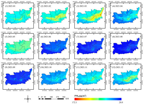
Figure A4.
Spatial distribution of the monthly average PM10 concentrations in 2021.
Figure A4.
Spatial distribution of the monthly average PM10 concentrations in 2021.
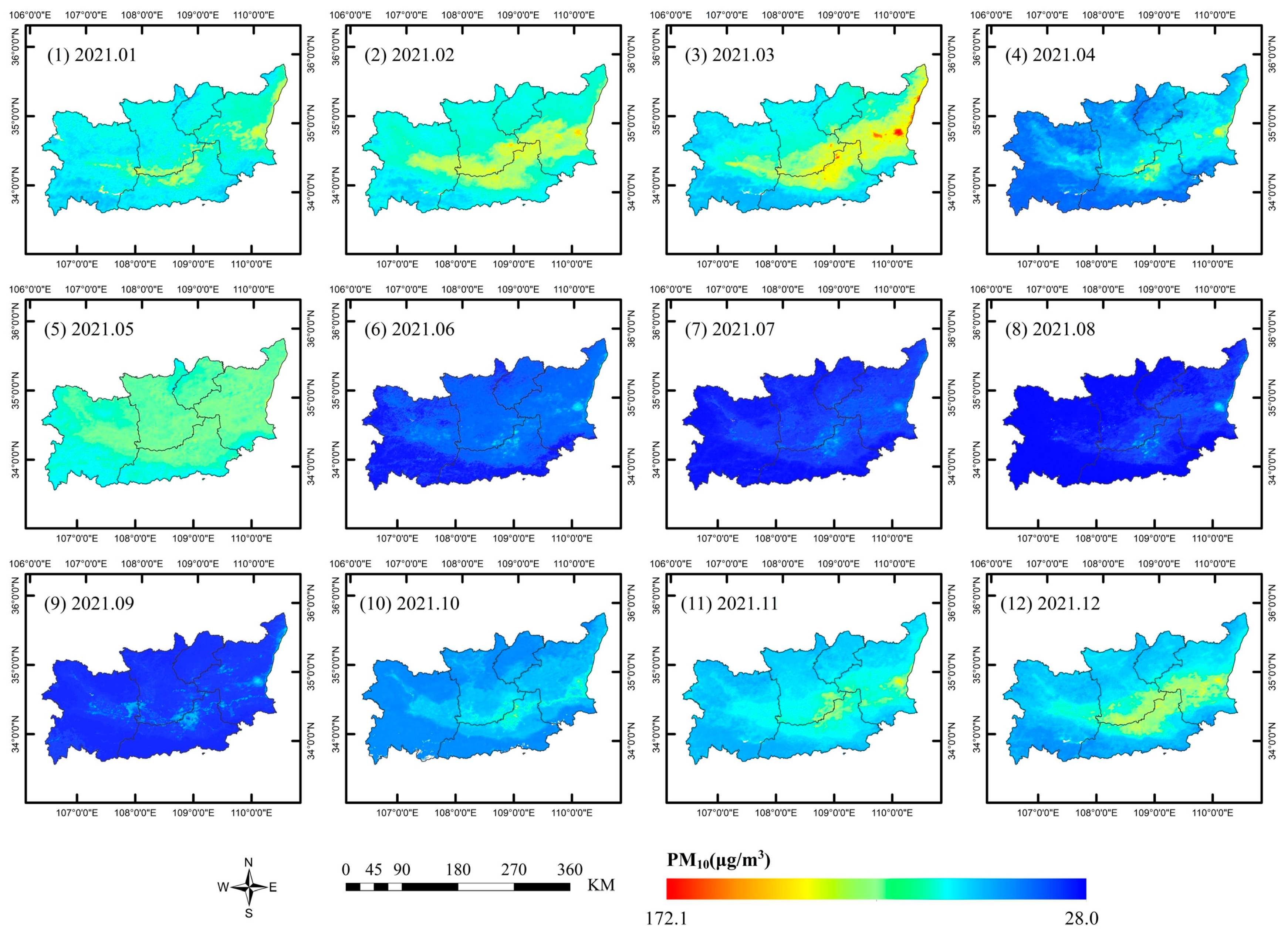
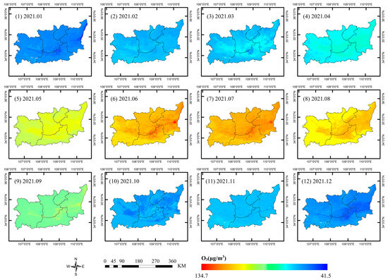
Figure A5.
Spatial distribution of the monthly average O3 concentrations in 2021.
Figure A5.
Spatial distribution of the monthly average O3 concentrations in 2021.
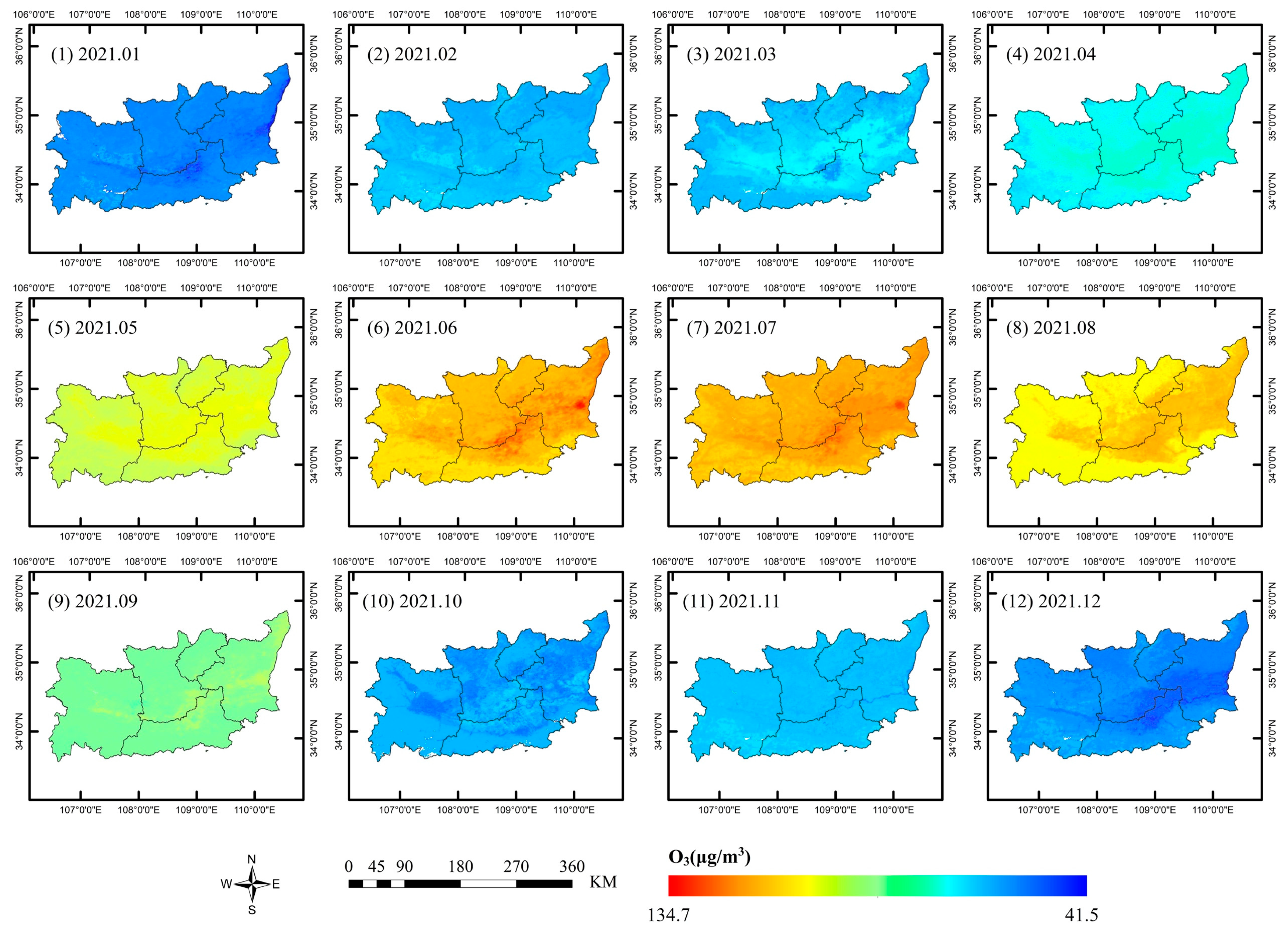
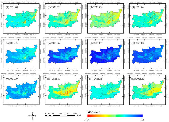
Figure A6.
Spatial distribution of the monthly average NO2 concentrations in 2021.
Figure A6.
Spatial distribution of the monthly average NO2 concentrations in 2021.
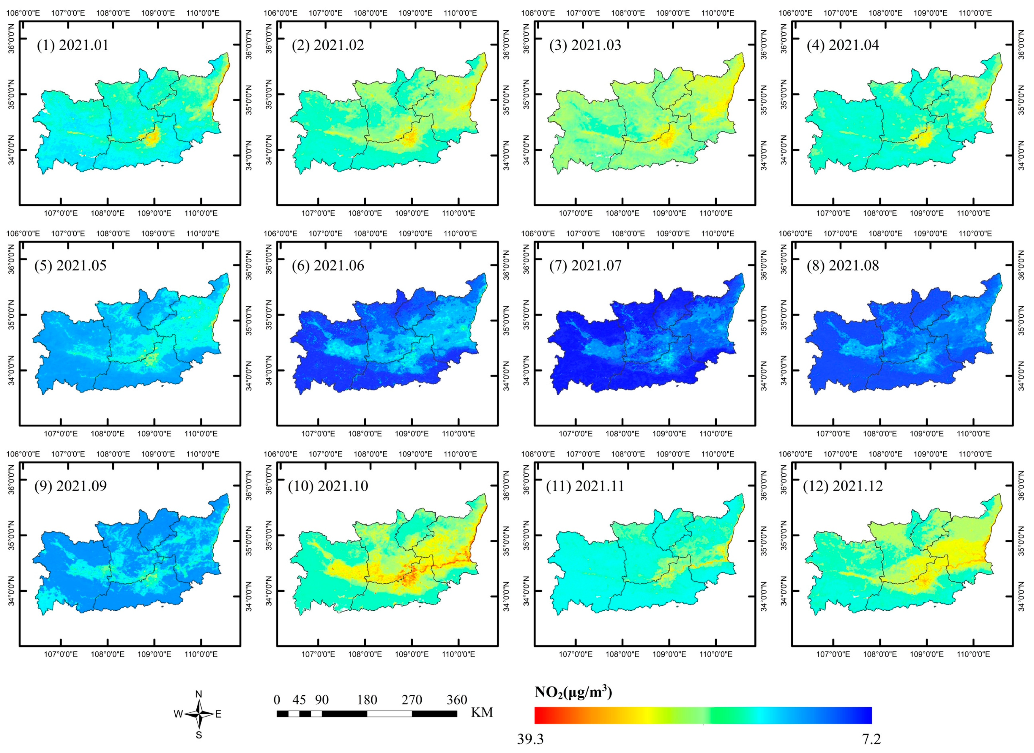

Figure A7.
Spatial distribution of the monthly average CO concentrations in 2021.
Figure A7.
Spatial distribution of the monthly average CO concentrations in 2021.
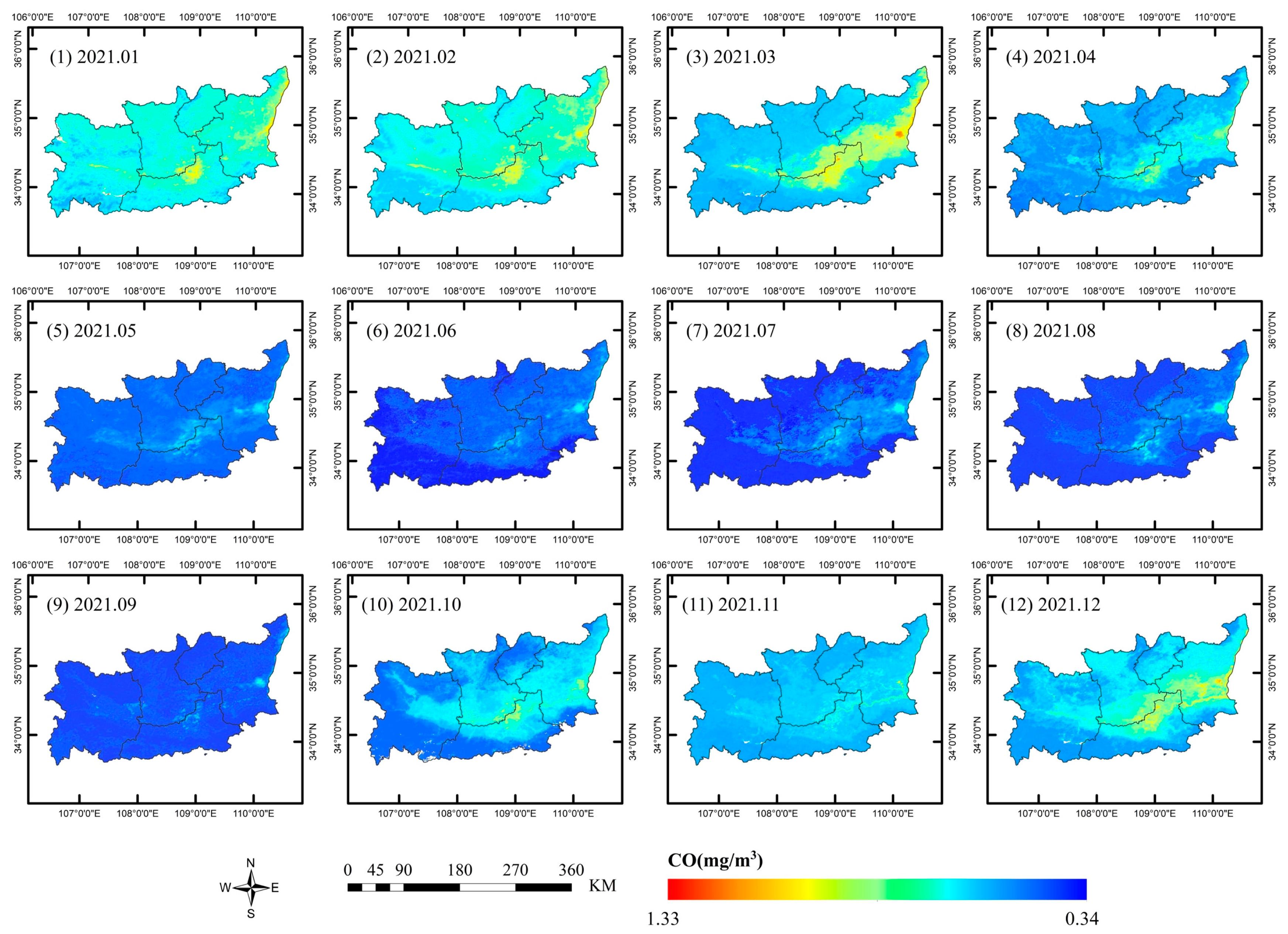
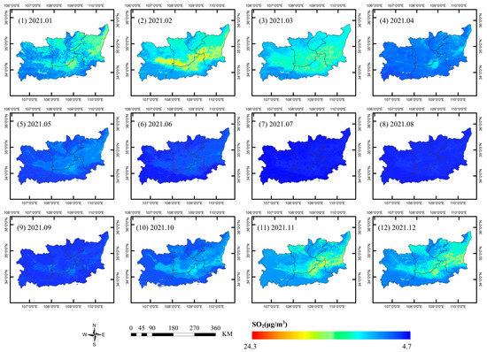
Figure A8.
Spatial distribution of the monthly average SO2 concentrations in 2021.
Figure A8.
Spatial distribution of the monthly average SO2 concentrations in 2021.

References
- Habre, R.; Moshier, E.; Castro, W.; Nath, A.; Grunin, A.; Rohr, A.; Godbold, J.; Schachter, N.; Kattan, M.; Coull, B.; et al. The effects of PM2.5 and its components from indoor and outdoor sources on cough and wheeze symptoms in asthmatic children. J. Expo. Sci. Environ. Epidemiol. 2014, 24, 380–387. [Google Scholar] [CrossRef] [PubMed]
- Guo, H.; Gu, X.; Ma, G.; Shi, S.; Wang, W.; Zuo, X.; Zhang, X. Spatial and temporal variations of air quality and six air pollutants in China during 2015–2017. Sci. Rep. 2019, 9, 15201. [Google Scholar] [CrossRef] [PubMed]
- Han, S.; Park, Y.; Noh, N.; Kim, J.-H.; Kim, J.-J.; Kim, B.-M.; Choi, W. Spatiotemporal variability of the PM2.5 distribution and weather anomalies during severe pollution events: Observations from 462 air quality monitoring stations across South Korea. Atmos. Pollut. Res. 2023, 14, 101676. [Google Scholar] [CrossRef]
- Wang, X.; Liu, M.; Luo, L.; Chen, X.; Zhang, Y.; Zhang, H.; Yang, S.; Li, Y. Spatial and Temporal Distributions of Air Pollutants in Nanchang, Southeast China during 2017–2020. Atmosphere 2021, 12, 1298. [Google Scholar] [CrossRef]
- Yuan, X.; Xia, Y.; He, J.; Cheng, M.; Qi, B.; Yu, Z.; Wang, B. Study on Accuracy Evaluation of MODIS AOD Products and Spatio-Temporal Distribution Characteristics of AOD in Hangzhou. Sustainability 2023, 15, 10171. [Google Scholar] [CrossRef]
- Liang, F.; Xiao, Q.; Wang, Y.; Lyapustin, A.; Li, G.; Gu, D.; Pan, X.; Liu, Y. MAIAC-based long-term spatiotemporal trends of PM2.5 in Beijing, China. Sci. Total Environ. 2018, 616-617, 1589–1598. [Google Scholar] [CrossRef]
- Zhang, Z.; Chang, L.Y.; Lau, A.K.H.; Chan, T.C.; Chieh Chuang, Y.; Chan, J.; Lin, C.; Kai Jiang, W.; Dear, K.; Zee, B.C.Y.; et al. Satellite-based estimates of long-term exposure to fine particulate matter are associated with C-reactive protein in 30 034 Taiwanese adults. Int. J. Epidemiol. 2017, 46, 1126–1136. [Google Scholar] [CrossRef]
- Wang, J.; Christopher, S.A. Intercomparison between satellite-derived aerosol optical thickness and PM2.5 mass: Implications for air quality studies. Geophys. Res. Lett. 2003, 30, 2095. [Google Scholar] [CrossRef]
- Engel-Cox, J.A.; Holloman, C.H.; Coutant, B.W.; Hoff, R.M. Qualitative and quantitative evaluation of MODIS satellite sensor data for regional and urban scale air quality. Atmos. Environ. 2004, 38, 2495–2509. [Google Scholar] [CrossRef]
- Zhang, T.; Zang, L.; Wan, Y.; Wang, W.; Zhang, Y. Ground-level PM2.5 estimation over urban agglomerations in China with high spatiotemporal resolution based on Himawari-8. Sci. Total Environ. 2019, 676, 535–544. [Google Scholar] [CrossRef]
- Qin, K.; Zou, J.; Guo, J.; Lu, M.; Bilal, M.; Zhang, K.; Ma, F.; Zhang, Y. Estimating PM1 concentrations from MODIS over Yangtze River Delta of China during 2014–2017. Atmos. Environ. 2018, 195, 149–158. [Google Scholar] [CrossRef]
- Su, T.; Li, J.; Li, C.; Lau, A.K.-H.; Yang, D.; Shen, C. An intercomparison of AOD-converted PM2.5 concentrations using different approaches for estimating aerosol vertical distribution. Atmos. Environ. 2017, 166, 531–542. [Google Scholar] [CrossRef]
- Mao, F.; Hong, J.; Min, Q.; Gong, W.; Zang, L.; Yin, J. Estimating hourly full-coverage PM2.5 over China based on TOA reflectance data from the Fengyun-4A satellite. Environ. Pollut. 2021, 270, 116119. [Google Scholar] [CrossRef]
- Shen, H.; Li, T.; Yuan, Q.; Zhang, L. Estimating Regional Ground-Level PM2.5 Directly From Satellite Top-Of-Atmosphere Reflectance Using Deep Belief Networks. J. Geophys. Res. Atmos. 2018, 123, 13875–13886. [Google Scholar] [CrossRef]
- Munchak, L.A.; Levy, R.C.; Mattoo, S.; Remer, L.A.; Holben, B.N.; Schafer, J.S.; Hostetler, C.A.; Ferrare, R.A. MODIS 3 km aerosol product: Applications over land in an urban/suburban region. Atmos. Meas. Tech. 2013, 6, 1747–1759. [Google Scholar] [CrossRef]
- Gupta, P.; Christopher, S.A. Particulate matter air quality assessment using integrated surface, satellite, and meteorological products: Multiple regression approach. J. Geophys. Res. Atmos. 2009, 114, D14205. [Google Scholar] [CrossRef]
- Yang, X.; Zhang, M.; Zhang, B. A Generic Model to Estimate Ozone Concentration From Landsat 8 Satellite Data Based on Machine Learning Technique. IEEE J. Sel. Top. Appl. Earth Obs. Remote Sens. 2021, 14, 7938–7947. [Google Scholar] [CrossRef]
- Brokamp, C.; Jandarov, R.; Hossain, M.; Ryan, P. Predicting Daily Urban Fine Particulate Matter Concentrations Using a Random Forest Model. Environ. Sci. Technol. 2018, 52, 4173–4179. [Google Scholar] [CrossRef]
- de Hoogh, K.; Heritier, H.; Stafoggia, M.; Kunzli, N.; Kloog, I. Modelling daily PM2.5 concentrations at high spatio-temporal resolution across Switzerland. Environ. Pollut. 2018, 233, 1147–1154. [Google Scholar] [CrossRef]
- Park, Y.; Kwon, B.; Heo, J.; Hu, X.; Liu, Y.; Moon, T. Estimating PM2.5 concentration of the conterminous United States via interpretable convolutional neural networks. Environ. Pollut. 2020, 256, 113395. [Google Scholar] [CrossRef]
- Yang, Q.; Yuan, Q.; Gao, M.; Li, T. A new perspective to satellite-based retrieval of ground-level air pollution: Simultaneous estimation of multiple pollutants based on physics-informed multi-task learning. Sci. Total Environ. 2023, 857, 159542. [Google Scholar] [CrossRef]
- Fisthtahler, L. Standard data products from the MODIS science team. Geosci. Remote Sens. 1996, 2820, 230–244. [Google Scholar]
- Chi, Y.; Shi, H.; Wang, X.; Qin, X.; Zheng, W.; Peng, S. Impact factors identification of spatial heterogeneity of herbaceous plant diversity on five southern islands of Miaodao Archipelago in North China. Chin. J. Oceanol. Limnol. 2016, 34, 937–951. [Google Scholar] [CrossRef]
- Lin, R.; Chen, H.; Wei, Z.; Li, Y.; Zhang, B.; Sun, H.; Cheng, M. Improved Surface Soil Moisture Estimation Model in Semi-Arid Regions Using the Vegetation Red-Edge Band Sensitive to Plant Growth. Atmosphere 2022, 13, 930. [Google Scholar] [CrossRef]
- Zhang, B.; Zhang, M.; Kang, J.; Hong, D.; Xu, J.; Zhu, X. Estimation of PMx Concentrations from Landsat 8 OLI Images Based on a Multilayer Perceptron Neural Network. Remote Sens. 2019, 11, 646. [Google Scholar] [CrossRef]
- Barenbrug, A.W.T. Psychrometry and Psychrometric Charts, 3rd ed.; Cape and Transvaal Printers Ltd.: Cape Town, South Africa, 1974. [Google Scholar]
- Wang, Z.; Zhang, M. Evaluation and Comparison of Different Machine Learning Models for NSAT Retrieval from Various Multispectral Satellite Images. Atmosphere 2022, 13, 1429. [Google Scholar] [CrossRef]
- Wu, Y.; Guo, J.; Zhang, X.; Tian, X.; Zhang, J.; Wang, Y.; Duan, J.; Li, X. Synergy of satellite and ground based observations in estimation of particulate matter in eastern China. Sci. Total Environ. 2012, 433, 20–30. [Google Scholar] [CrossRef]
- Lee, S.; Choeh, J.Y. Predicting the helpfulness of online reviews using multilayer perceptron neural networks. Expert. Syst. Appl. 2014, 41, 3041–3046. [Google Scholar] [CrossRef]
- Tarvainen, T.; Vauhkonen, M.; Kolehmainen, V.; Arridge, S.R.; Kaipio, J.P. Coupled radiative transfer equation and diffusion approximation model for photon migration in turbid medium with low-scattering and non-scattering regions. Phys. Med. Biol. 2005, 50, 4913–4930. [Google Scholar] [CrossRef]
- Wang, S.-T. Optimized Light Guide Plate Optical Brightness Parameter: Integrating Back-Propagation Neural Network (BPN) and Revised Genetic Algorithm (GA). Mater. Manuf. Process. 2014, 29, 1–8. [Google Scholar] [CrossRef]
- Mishra, P.K.; Karmakar, S. Performance of back-propagation neural network in chaotic data time series forecasting and evaluation over parametric forecast: A case study for rainfall-runoff modelling over a river basin. Int. J. Inf. Technol. 2018, 15, 917–935. [Google Scholar] [CrossRef]
- Hong, J.; Mao, F.; Min, Q.; Pan, Z.; Wang, W.; Zhang, T.; Gong, W. Improved PM2.5 predictions of WRF-Chem via the integration of Himawari-8 satellite data and ground observations. Environ. Pollut. 2020, 263, 114451. [Google Scholar] [CrossRef] [PubMed]
Disclaimer/Publisher’s Note: The statements, opinions and data contained in all publications are solely those of the individual author(s) and contributor(s) and not of MDPI and/or the editor(s). MDPI and/or the editor(s) disclaim responsibility for any injury to people or property resulting from any ideas, methods, instructions or products referred to in the content. |
© 2024 by the authors. Licensee MDPI, Basel, Switzerland. This article is an open access article distributed under the terms and conditions of the Creative Commons Attribution (CC BY) license (https://creativecommons.org/licenses/by/4.0/).