Integrated Predictive Modeling and Policy Factor Analysis for the Land Use Dynamics of the Western Jilin

Abstract

The external environment in the transitional zone of the ecological barrier is fragile, and economic growth has resulted in a series of land degradation issues, significantly impacting regional economic development and the ecological environment. Therefore, monitoring, assessing, and predicting land use changes are crucial for ecological security and sustainable development. This study developed an integrated model comprising convolutional neural network, cellular automata, and Markov chain to forecast the land use status of western Jilin, located in the transitional zone of the ecological barrier, by the year 2030. Additionally, the study evaluated the role of land use policies in the context of land use changes in western Jilin. The findings demonstrate that the coupled modeling approach exhibits excellent predictive performance for land use prediction in western Jilin, yielding a Kappa coefficient of 93.26%. Policy drivers play a significant role in shaping land use patterns in western Jilin, as evidenced by the declining farmland accompanied by improved land utilization, the sustained high levels of forest aligning with sustainable development strategies, the ongoing restoration of waters and grassland, which are expected to show positive growth by 2030, and the steady growth in built-up areas. This study contributes to understanding the dynamics of land use in the transitional zone of the ecological barrier, thereby promoting sustainable development and ecological resilience in the region.

1. Introduction

Constructing ecological civilization is a crucial strategy for ensuring sustainable development for humanity [1]. China has established the “two barriers and three belts” ecological security strategy framework, with a focus on regional resources, environment, and economy, to facilitate the systematic and well-organized assessment of future changes in surface ecological patterns. The primary objectives of the framework are to protect national ecological security and accomplish key milestones in sustainable development [2,3]. However, the transitional zones of the Northeast Forest belt and the Northern Sand prevention belt, located in the forest–grassland–desert transition belt, exhibit unstable internal structures and vulnerable external environments due to factors such as low precipitation and frequent wind and sandstorms [4,5]. Driven by economic interests, grasslands and wetlands have been extensively reclaimed for agricultural purposes, leading to land degradation. Moreover, the extensive cultivation of low-yield lands is a primary cause of desertification in the region [5]. The irrational land use patterns and lack of coordination in land utilization have particularly severe impacts on regional economic development and the ecological environment. Facing significant risks posed by global climate change and rapid economic development, as well as the multitude of complex ecological challenges, there is notable spatiotemporal uncertainty [6,7]. These challenges have significantly impeded the development of ecological projects and the formulation of related policies.

Located in the transitional belt of ecological barriers, the western part of Jilin Province presents a typical case with complex land use types. With the rapid advancement of industrialization and urbanization, the demand for various functional lands has increased, leading to a higher utilization intensity of land resources. Consequently, conflicts and contradictions arise among the different types of land use, resulting in an imbalanced spatial structure, which will significantly impact both the national land spatial pattern and regional sustainable development [8]. Resolving land use conflicts has become one of the urgent and critical issues. To address the challenges posed by global climate change, urbanization, and human activities, the Chinese government and local authorities have implemented a range of policies aiming to rationalize the utilization of the limited land resources [9,10,11,12,13]. Considering the complex and uncertain nature of land use issues, developing a probabilistic model that incorporates temporal and spatial factors can partially predict future trends in western Jilin, evaluate the appropriateness of current or related policies, analyze the synergistic relationship between land use and policies, and offer a scientific basis for future decision-making processes. This can promote regional ecological security and sustainable development, which is highly important and valuable for achieving green and sustainable development in the rapidly developing, human–environment-conflicting, and ecologically fragile western Jilin.

Several models have been developed for land use prediction, including the gray model [14]; the conversion of land use and its effects at small regional extent model [15]; the cellular automata model (CA) [16,17]; the Markov chain model (MC) [18]; the logistic regression model [19]; the SimWeight model [20]; the slope, land use, exclusion, urbanization, transportation and hillshade model [21]; the support vector machine model [22]; the land transformation model [23]; and the convolutional neural network model (CNN) [24]. The CA model can simulate the spatiotemporal evolution of various natural processes in a flexible and simple manner, reflecting the local interactions of system evolution dynamics. However, it heavily depends on spatial data and is constrained by the technical limitations of a single model [25]. The MC model is effective in simulating long-term quantity trends but does not fully consider spatial parameters, thus being unable of capturing the spatial variability in land use [18]. To overcome these limitations, some studies have modified and integrated the CA model into the MC model, resulting in the CA-MC model. This integrated model monitors the spatiotemporal changes in land use types by utilizing the transition matrix [26,27], in which the MC model controls the temporal changes [18] and the CA model’s spatial filter controls the spatial changes [28].

While the potential of the CA-MC model has been recognized, the driving factors to be considered in realistic simulations are highly complex. Therefore, integrating them into other models may be one effective approach to enhance the understanding of evolutionary patterns and improve predictive capabilities [26,29]. The CNN model, among the powerful artificial intelligence (AI) models, can effectively handle complex nonlinear relationships and high-dimensional data. However, it has limitations in terms of model interpretation and generalization ability [30]. In comparison, the CNN model can address the CA model’s deficiencies in neglecting the influence of macro-factors on the process; the CA and MC models can address the slow convergence, susceptibility to local minima, and challenges in determining the network structure of the CNN model [31,32]. Given the significance of the potential of the CA, MC, and CNN models, this study aims to develop a coupled CNN-CA-MC model for predicting the land use scenario of the western Jilin in 2030 and validate the rationality of the current policies, explore future policy trends and directions, and provide the support of theoretical foundation for the western Jilin land use planning and sustainable land resource development, thus promoting the sustainable utilization of land resources and the preservation of the ecological environment.

The paper is structured as follows. Section 2 provides the location of the study area, the database, the data preparation process, and the coupling method of the model. Section 3 presents the results of the land use change prediction for 2030 and analyzes the factors driven by policies. The discussion and conclusion are provided in Section 4 and Section 5, respectively.

2. Materials and Methods

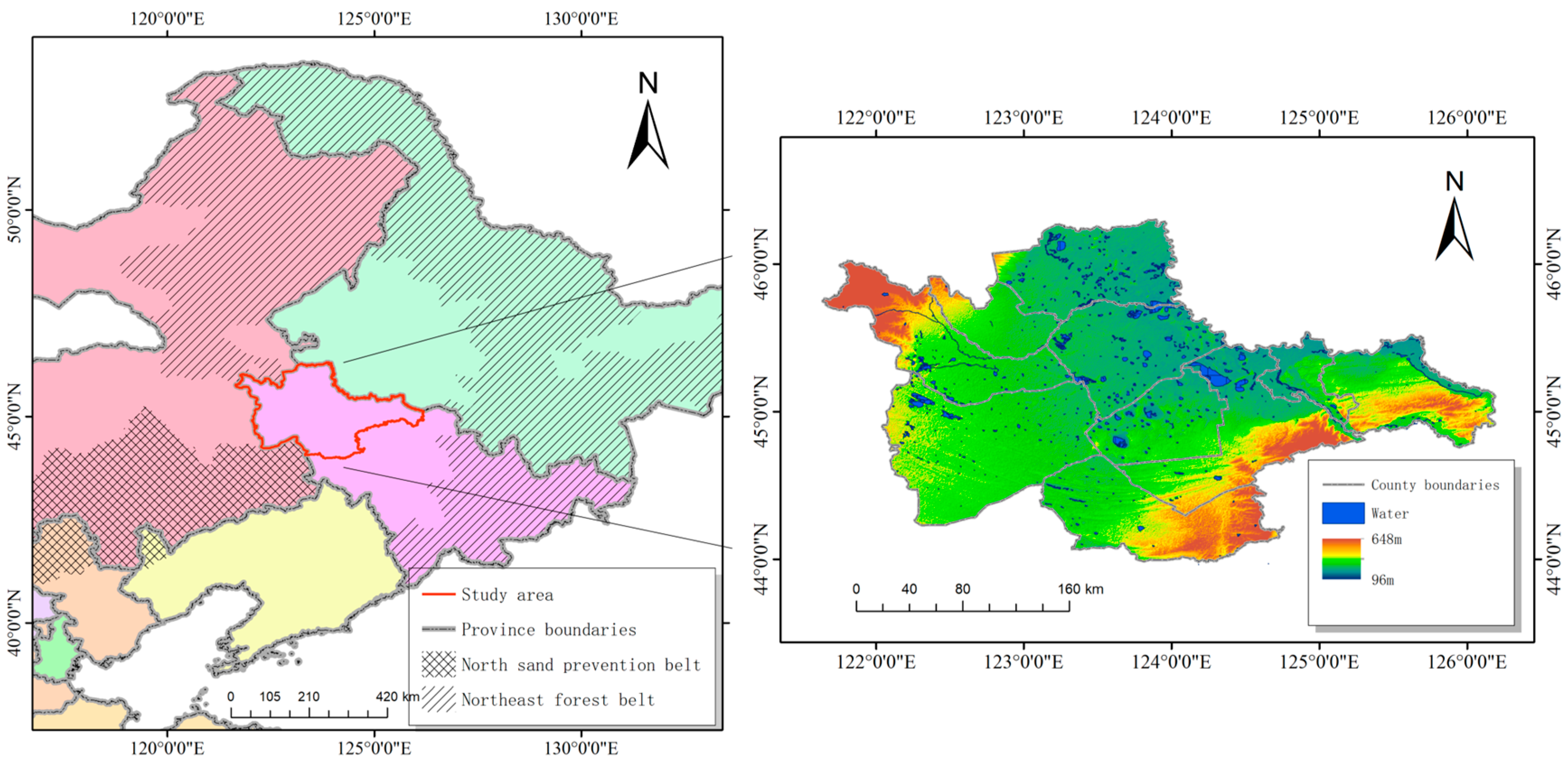
2.1. Study Area

The western of Jilin Province, spanning 121.38° E–126.11° E and 43.59° N–46.18° N, covers an approximate total area of 48,000 km² (Figure 1). It is located in the transitional area between the northeast forest zone and the northern sand prevention zone, characterized by a mosaic of low-lying, easily waterlogged saline–alkali and sandy areas, making the ecological environment extremely fragile. The administrative region includes two prefecture-level cities, Baicheng and Songyuan, with 10 county-level administrative divisions. The area is higher in the east, south, and west, while the northern and central parts are relatively lower, with elevations in the range of 96–648 m. The region is prone to risks, such as erosion and inadequate drainage. The average annual temperature ranges from 4 to 5 °C, and the annual rainfall varies between 400 and 500 mm, decreasing from the eastern to the western plains, with precipitation being significantly lower than evaporation. The area is located in the transitional zone between agriculture and animal husbandry in northern China, characterized as a typical semi-arid to semi-humid region. It faces severe issues, such as soil salinization, desertification, grassland degradation, wetland shrinkage, and irrational land use structures [33]. With rapid industrialization and urbanization, there is an increasing demand for different types of land and an intensification of land resource utilization. Consequently, conflicts and contradictions arise between different land use types, leading to an imbalanced land spatial structure. Therefore, this region is a focal point for our study, as it stands to benefit from the findings of our research.

2.2. Dataset and Preprocessing

Land use and land cover change (LUCC) is influenced by a multitude of natural, economic, and human factors. According to the principles of scientific rigor, representativeness, and systematic approach, the dataset and sources used in this study are presented in

Table 1. A sketch of the utilized geospatial and attribute data.

	Data	Type	Year	Resolution	Resource
1	Land use dataset	Raster	2000, 2010, 2020	30 m	https://www.resdc.cn/ (accessed on 15 December 2023)
2	GDEM V3	Raster	2000~2013	30 m	https://www.earthdata.nasa.gov/ (accessed on 15 December 2023)
3	Distance to water	Raster	2000, 2010, 2020	30 m	Calculated from Land use dataset
4	Reservoir	Raster	2000, 2010, 2020	30 m	Reclass from Land use dataset
5	Slope	Raster	2000~2013	30 m	Calculated from GDEM V3
6	Policy constraint factors	Raster	2000~2013	30 m	Manual statistics

. The primary land use monitoring data for this study were obtained from the Resource and Environmental Science Data Center, covering 3 periods (2000, 2010, and 2020). These data were generated by the Institute of Geographic Sciences and Natural Resources Research, Chinese Academy of Sciences, utilizing Landsat 8 remote sensing images as the primary information source. The data underwent rigorous professional processing, including radiometric and geometric corrections, with an accuracy of ≥90% [34]. Land use types were reclassified into 6 primary categories (farmland, forest, grassland, water, built-up area, and undeveloped land) based on the classification standard of the Chinese Academy of Sciences Land Resource Classification System [35,36,37].

GDEM V3 is a high-resolution elevation data covering the global land surface, which was derived from the Advanced Spaceborne Thermal Emission and Reflection Radiometer (ASTER). The Ministry of Economy, Trade, and Industry (METI) and the National Aeronautics and Space Administration (NASA) collaborated on its development. The distance to water data were derived by applying the Distance tool in IDRISI Sleva 17.0 [38,39,40] to the reclassed land use monitoring data. The reservoir data were also extracted from the reclassified land use monitoring data and used to generate and correct the suitability maps. The slope data were derived from GDEM V3. Given that the areas in proximity to water, characterized by lower DEM values and gentler slopes, are more conducive to plant growth and human activities, the distance from water, DEM, and slope data were reverse normalization. Moreover, the Chinese government has implemented regulations prohibiting the cultivation of land with slopes greater than 25° and granting special protection for forests with slopes greater than 25°, which have a profound influence on changes in ecological layout; hence, we considered it as a policy control factor. Considering that the number of agricultural land pixels in the study area was much greater than the number of forest land pixels and the number of pixels with slopes lower than or equal to 25° was much greater than the number of pixels with slopes greater than 25°, when reclassifying the slope data, we set the pixel values greater than 25° to 0 and the pixel values lower than or equal to 25° to 1, serving as a constraint factor for prediction and control.

The data underwent preprocessing, including projection unification, clipping, and calibration. The nearest-neighbor method was employed for resampling discrete data, whereas bilinear interpolation was utilized for resampling the continuous data. The final spatial resolution of all raster data was standardized to 30 m/pixel in the Krasovsky_1940_Albers (ESPG: 7024) coordinate system.

2.3. Methods

The specific process and input data in this study are shown in Figure 2 and

Table 2. Input dataset.

Name	Input 1		Input 2	Input 3	Input 4
	Input 1-1	Input 1-2
Dataset A	2000_11 and 2010_6	2010_11	2000_11 and 2010_6	2010_6	2020_6
Dataset B	2010_11 and 2020_6	2020_11	2010_11 and 2020_6	2020_6	-

, respectively. As shown in Table 2, the first 4 digits represent the year and the suffix “_11” denotes the inclusion of a total of 11 types of datasets, encompassing 6 types of land use (farmland, forest, grassland, water, built-up area, and undeveloped land), reservoir, distance from water, DEM, slope, and policy factor data. The suffix “_6” indicates the inclusion of only 6 types of land use data. Dataset A represents the data used to predict land use in 2020, whereas dataset B represents the data used to predict land use in 2030. During the prediction, dataset A was first fed into the model, and input 1 and input 2 served as the parameters to calculate the transfer probability matrix and suitability maps through the spatial transfer rule module and quantity transfer rule module, respectively. The resulting transfer probability matrix, suitability maps, and input 3 were collectively employed as parameters in the CA model. The prediction results were subsequently calibrated and compared to input 4. If the evaluation indicated that the model met the prediction requirements, the dataset B was used to predict land use changes in 2030. Detailed information on the specific module descriptions and computational processes are provided in the following sections.

In this study, the CA and MC models were implemented using IDRISI Sleva 17.0 and the CNN model was made using PaddlePaddle 2.3.2 with the interpreter CPython 3.10.12.

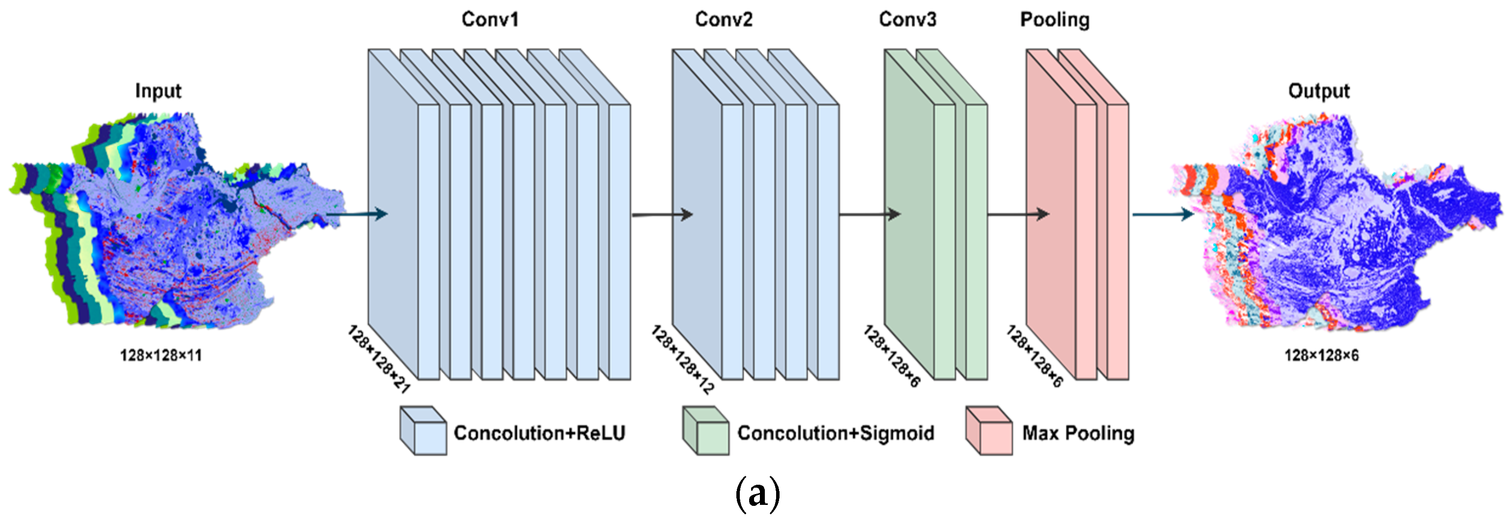
2.3.1. Spatial Transfer Rule and Convolutional Neural Network

The CNN, correct, and stretch steps were performed successively to obtain the suitability maps for the spatial transfer rule (Figure 2). The essence of the CNN model lies in the utilization of convolutional operations and pooling operations to achieve end-to-end training and classification and map the relationship from the input to the output [41].

A CNN model’s basic structure comprises an input layer, convolutional layers, activation function layers, pooling layers, fully connected layers, and an output layer [42]. Among these components, the convolutional layers are the core of the CNN. They perform convolution operations on input images using learnable convolution kernels, extracting features and capturing the spatial local relationships. Activation functions introduce nonlinearity and enhance the model’s expressiveness. Rectified linear unit (ReLU (1)) and sigmoid (2) can be applied to extract nonlinear features after each convolutional layer [43]. Pooling layers are used to reduce the spatial dimensions of feature maps, thereby reducing the computational complexity and extracting more prominent features. The fully connected layer transforms the feature maps into classification or regression outputs and is typically placed at the end of the convolutional neural network. It flattens the feature maps into a one-dimensional vector that is subsequently utilized for classification or regression predictions. The training of a CNN model commonly employs the backpropagation algorithm to optimize the model parameters by minimizing the loss function. During training, the CNN model can automatically learn features from the images without the need for manual feature extractors because fully connected layers can cause the loss and confusion of spatial information, this study did not include them.

$$\mathrm{ReLU}:f\left(x\right)=\max \left(0,x\right)$$

(1)

$$\mathrm{Sigmoid}:f\left(x\right)=\frac{1}{1+e^{-x}}$$

(2)

The CNN model in this study comprised 3 convolutional layers (Conv1, Conv2, and Conv3) and an adaptive max pooling layer (Figure 3a). Conv1 had 11 input channels and 21 output channels, Conv2 had 21 input channels and 12 output channels, and Conv3 had 12 input channels and 6 output channels. The kernel size for all convolutional layers was 3 × 3, with a stride of 1, and reflection padding was applied with a padding size of 1. ReLU was employed as the activation function after the first two convolutional layers (Conv1 and Conv2), whereas Sigmoid was used after the third convolutional layer (Conv3). Finally, the feature map size was adjusted to 128 × 128 through the adaptive max pooling layer.

The input layer parameters consisted of 6 types of land use data, DEM, distance from water, reservoir, slope, and policy control factor data. After partitioning the original data, the image was divided into multiple sub-images of 128 × 128 size, which were then used as input for training the constructed CNN model, which utilized 11 channels. During the forward propagation, the input data underwent convolution and adaptive max pooling operations, generating output data with 6 channels. Subsequently, the mean squared error was used as the loss function to compute the loss value. During the backward propagation, the Adam optimizer was used to compute the weights gradients and update the weights, thereby facilitating gradient descent. By performing multiple iterations and weight optimization, the best accuracy was achieved. Finally, the suitability maps were obtained by stitching the processed individual input images.

Taking dataset A as an example, the input 1-1 data was cropped into a size of 128 × 128, resulting in the generation of a dataset. Subsequently, the dataset was split into a training set and a validation set at an 8:2 ratio. Training was conducted on the training set, and the loss was computed by comparing the predicted results with the actual classification results (Figure 3b). Once the loss value on the validation set no longer decreased, input 1-2 was fed into the CNN model for prediction, generating a suitability map for 2010. After correcting the results obtained from the CNN operation, the grid values were scaled to the range from 0 to 255 while maintaining integer values. At this stage, the spatial transfer rule module finished its operation. The same procedure was applied to dataset B, where the input data from the years 2010 and 2020 were utilized to generate a suitability map for 2020.

2.3.2. Quantity Transfer Rules and Markov Chain Model

The MC model, which is a theory based on the process of the formation of Markov random process systems for the prediction and optimal control theory method, is utilized to calculate the quantity transfer rules, resulting in the generation of a transfer probability matrix and a transfer area matrix [44]. It is commonly used to predict geographical characteristics, especially in scenarios without an aftereffect event, making it a crucial method in geographic research. The prediction of land use changes is calculated using the conditional probability formula [17,45,46]:

$$S_{t+1}=P_{i,j}\times S_t$$

(3)

where $S_t$ and $S_{t+1}$ are the system status at the times of $t$ and $t+1$, respectively; and $P_{i,j}$ is the transition probability matrix in a state, which is calculated as follows:

$$P_{i,j}=\begin{array}{ccc}{P}_{11}& \dots & P_{1n}\\ ⋮& \ddots & ⋮\\ P_{n1}& \dots & P_{nn}\end{array},0\le P_{i,j}\le 1\mathrm{and}{\sum }_{j=1}^n{P}_{i,j}=1(i,j=1,2,\dots n)$$

(4)

2.3.3. Cellular Automata Model

The CA model is a dynamic system that evolves and simulates spatial and temporal processes based on a cell space and specific rules, which is characterized by discrete time, discrete space, and discrete states, where each variable can only take a finite number of states. The transition rules of the CA model are local in both time and space [47,48]. Its primary application is to describe discrete dynamic systems in spatial contexts. The CA model can be represented as:

$$A=\left(L_d,S,N,F\right)$$

(5)

where $A$ represents the CA model, $L_d$ represents the cell space in a d-dimensional cellular automaton, $S$ represents the set of all cell states, $N$ represents the neighborhood state of the central cell, and $F$ represents the transition rules.

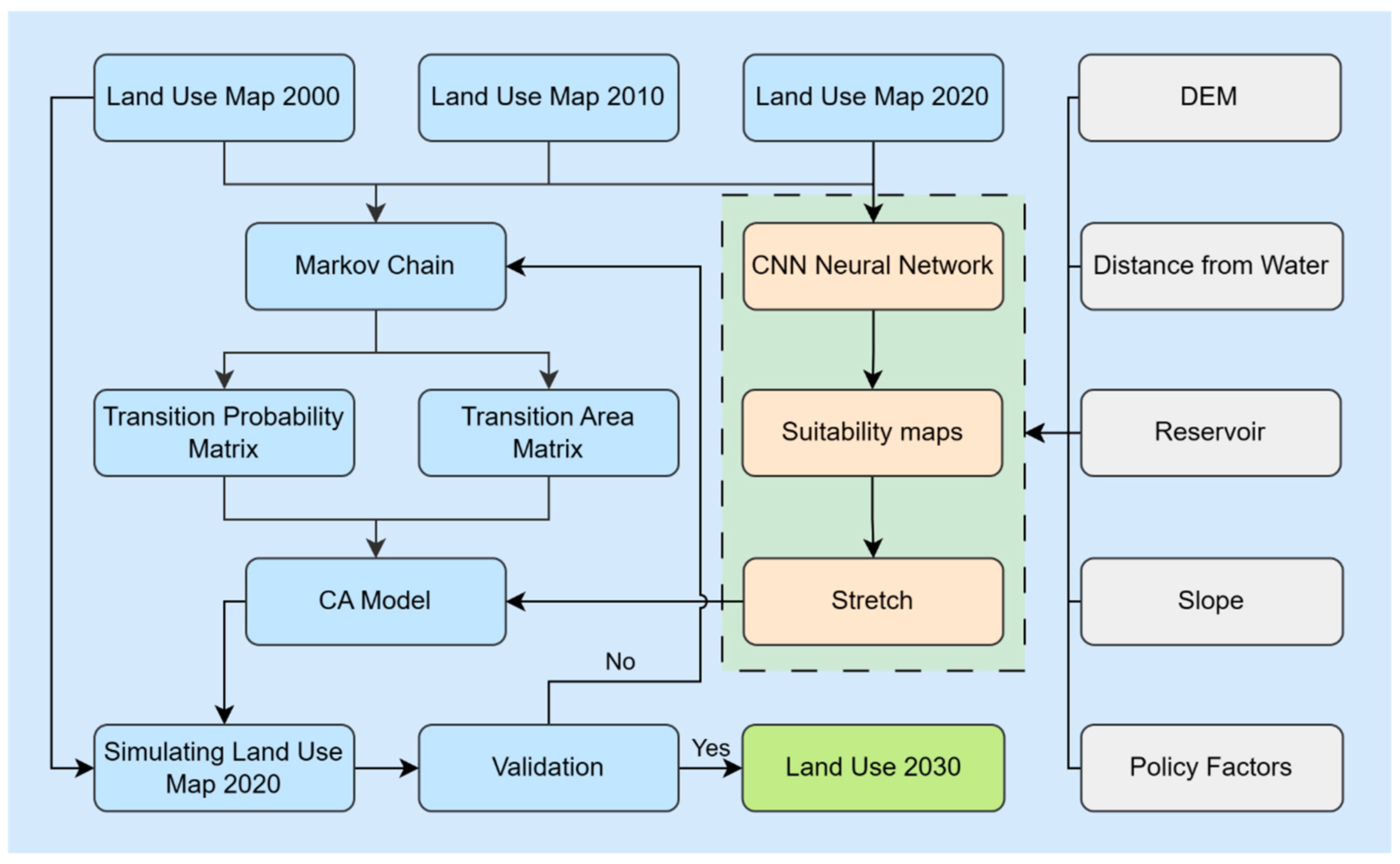
2.3.4. CNN-CA-MC Model and Accuracy Assessment

The CNN-CA-MC model builds upon the foundation of the CA model, integrating crucial components from the MC and CNN models. The construction of this model involves the following elements:

• Each grid with a spatial resolution of 30 × 30 m represents and stores the land use state, forming the cells. These cells collectively constitute the cellular space, distributed in spatial space.
• Each grid has an attribute known as the state, representing the land use type.
• The neighborhood concept employs a 5 × 5 Moore-type configuration, including the central cell and its 24 surrounding cells. It considers the influence of the surrounding cells on the attributes of the central cell.
• The transition rule governs the state of the neighborhood at the subsequent time step based on the current state of the cell and the condition of the neighborhood. It is defined as follows:

$$f:S_i^{t+1}=f\left(S_i^t{,S}_N^t\right)$$

(6)

where $f$ represents the transition rule, which comprises both quantity transition rules (derived from the transition probability matrix computed using the MC model) and spatial transition rules (generated by the CNN model in the form of suitability maps). $S_i^{t+1}$ denotes the state of cell $i$ at time $t+1$, $S_i^t$ represents the state of cell $i$ at time $t$, and $S_N^t$ represents the combined state of the neighborhood of cell $i$ at time $t$.

5.

The CA model evolves in discrete time steps. In this context, discrete time refers to the iteration count or time interval at which the CA model progresses. For this specific case, the iteration count aligns with the 10-year interval between the utilized basic data, resulting in a specified iteration count corresponding to a 10-year interval.

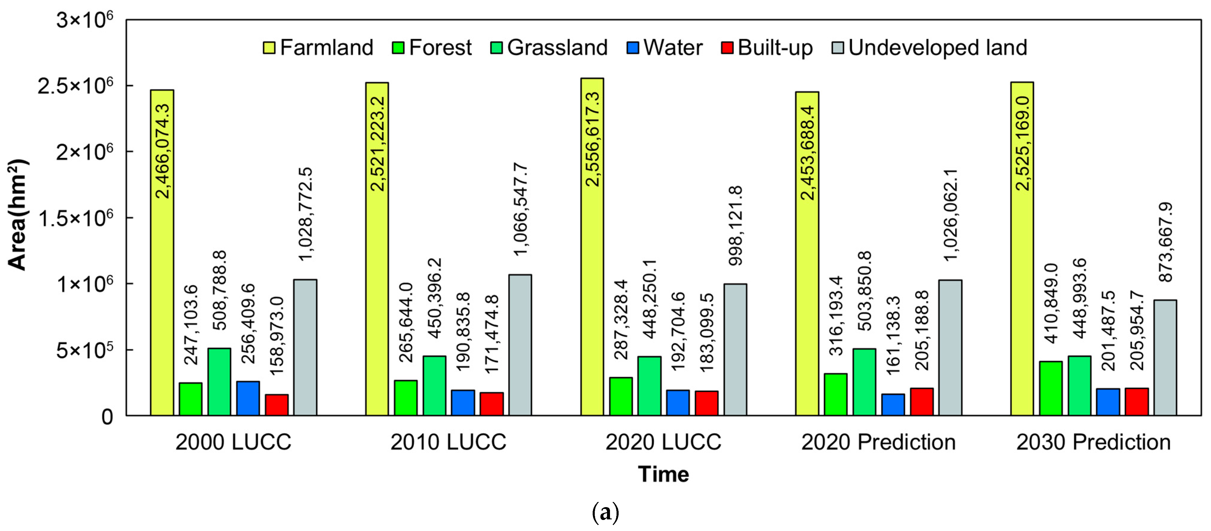
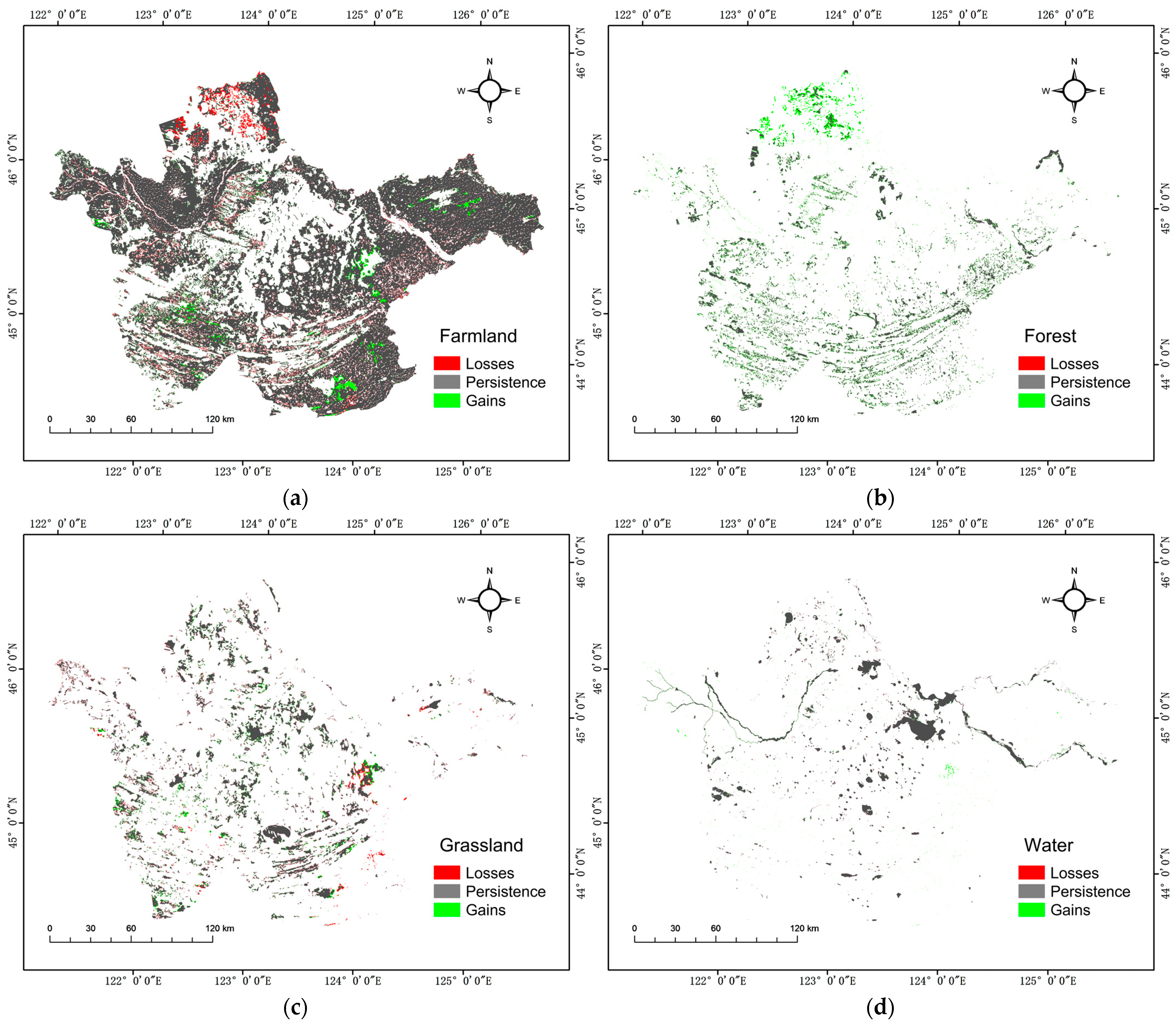
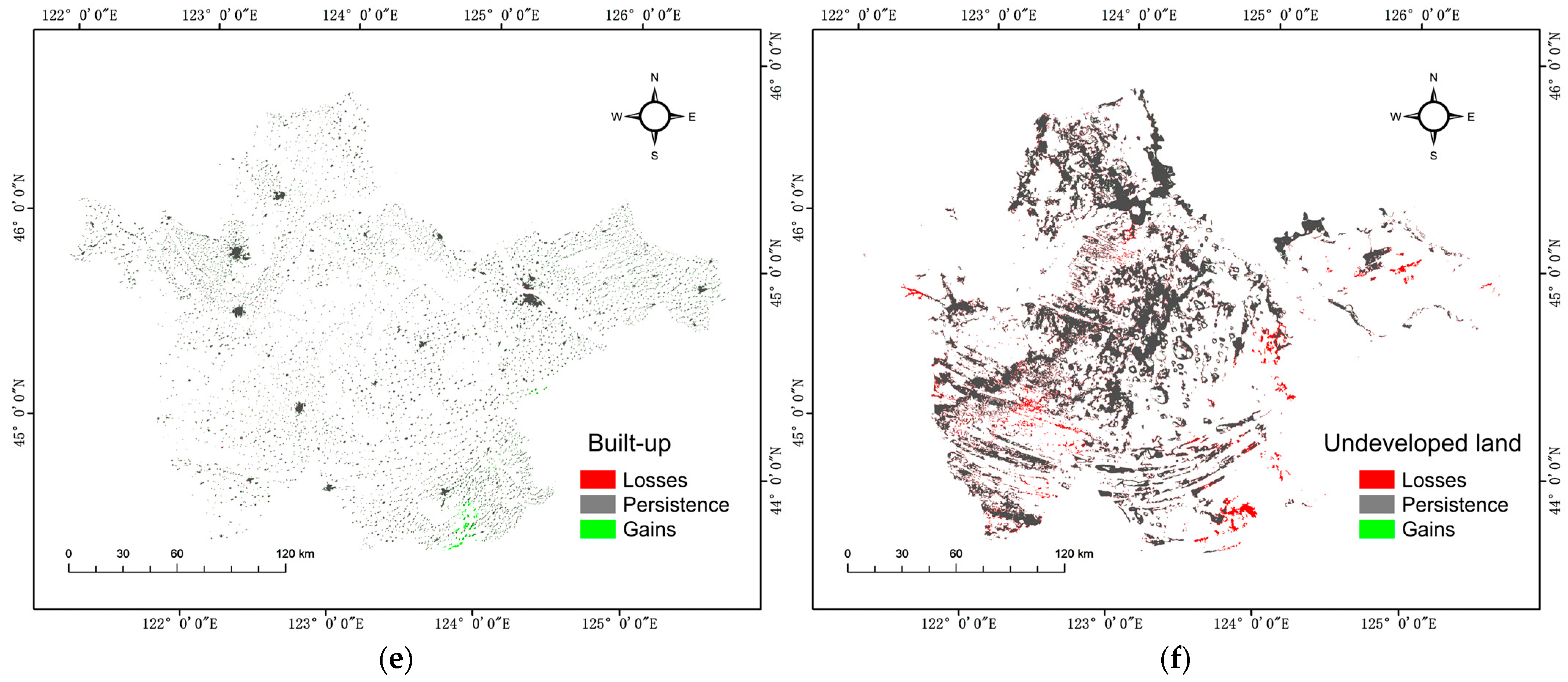
The CNN-CA-MC coupled model was validated for its accuracy by comparing the predicted land use results with the actual land use outcomes and calculating the $Kappa$ coefficient. A satisfactory level of accuracy is typically indicated by a $Kappa$ coefficient greater than 0.75 or 0.8 [49,50]. The computation of the $Kappa$ coefficient is as follows:

$$Kappa=\frac{P_0-P_c}{1-P_c}$$

(7)

where $P_0$ represents the proportion of correctly simulated cells and $P_c$ denotes the expected proportion of simulated cells.

3. Results

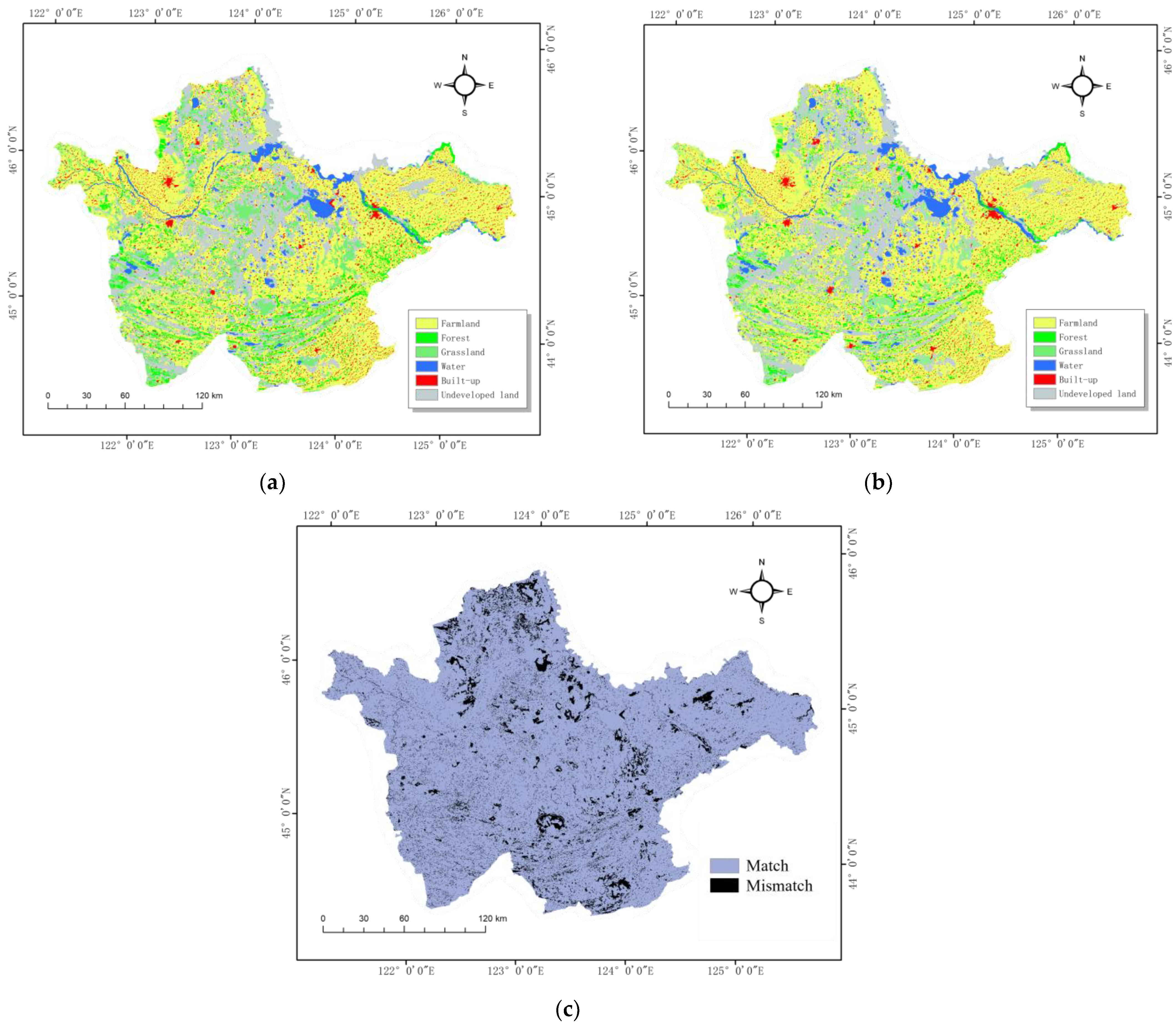
3.1. CNN-CA-MC Simulation

To further validate the accuracy of the model, the optimized CNN-CA-MC model was employed to predict land use firstly for 2020. The results of the transition area (probability) matrix indicate the likelihood of land use types transitioning to other land use types (

Table 3. Transition area (probability) matrix of the period from 2010 to 2020 (hm²).

	Farmland	Forest	Grassland	Water	Built-Up Area	Undeveloped Land
Farmland	1,325,715.1 (76.6%)	103,360.7 (6.0%)	112,233.5 (6.5%)	30,448.6 (1.8%)	63,766.6 (3.7%)	94,599 (5.5%)
Forest	53,769.8 (20.2%)	178,813.1 (67.3%)	17,693.0 (6.7%)	3536.3 (1.3%)	2540.9 (1%)	9290.9 (3.5%)
Grassland	111,277.9 (24.7%)	15,258.0 (3.4%)	243,024.4 (54%)	1513.6 (0.3%)	3055.1 (0.7%)	76,267.3 (16.9%)
Water	8085.2 (4.2%)	7820.8 (4.1%)	7061.5 (3.7%)	99,482.2 (52.1%)	1411.1 (0.7%)	66,974.9 (35.1%)
Built-up area	39,601.8 (23.1%)	2257.0 (1.3%)	2758.9 (1.6%)	333.9 (0.2%)	122,435.9 (71.4%)	4087.4 (2.4%)
Undeveloped land	115,745.3 (10.9%)	8682.5 (0.8%)	121,081 (11.4%)	34,216.3 (3.2%)	11,981.4 (1.1%)	774,841.1 (72.7%)

). It presents the probabilities of conversion between different land use types. For example, 76.6% of farmland was expected to remain unchanged, but there was a 6.5% probability of conversion to grassland, corresponding to an anticipated area change of 112, 233.5 hm². The area transition matrix also documented the pixels where specific land use and land cover changes occurred within the designated period. The comparison showed a good overall agreement between the predicted results and the actual distribution of land cover, with satisfactory predictions in terms of specific details (Figure 4). However, certain localized patches exhibited simulation errors, which could be attributed to the incomplete identification of the influencing factors or sudden impacts introduced by certain factors during the land use change process, such as policy interventions. Overall, the validated results of the CNN-CA-MC model show an impressive Kappa value of 93.26%, indicating a satisfactory performance for the simulation model. Additionally, the comparison of individual land cover areas showed a high degree of similarity.

In general, the coupled predictions of land use for the year 2020 using the CNN, CA, and MC models demonstrated relatively accurate simulation results, which can be utilized for predictive research. Before predicting the land use situation in the study area for 2030, it is necessary to adjust and modify the model parameters based on the 2020 data from the study area (Section 2.2). Correspondingly, the corresponding calculated transition area (probability) for each land use type from 2020 to 2030 is presented in

Table 4. Transition area (probability) matrix of the period from 2020 to 2030 (hm²).

	Farmland	Forest	Grassland	Water	Built-up Area	Undeveloped Land
Farmland	1458 (81.2%)	180.1 (10.0%)	27.5 (2.5%)	12.6 (0.7%)	64.4 (3.6%)	41.5 (2.3%)
Forest	68.4 (21.4%)	238.8 (74.8%)	2.3 (0.7%)	4.3 (1.4%)	1.1 (0.3%)	4.4 (1.4%)
Grassland	68.2 (13.7%)	11.1 (2.2%)	387.3 (77.8%)	7.6 (1.5%)	3.8 (0.8%)	20.1 (4.0%)
Water	6.4 (3.0%)	3.2 (1.5%)	2.4 (1.1%)	165.5 (77.3%)	0.3 (0.1%)	36.4 (17.0%)
Built-up area	26.3 (12.9%)	2.3 (1.1%)	1.5 (0.7%)	5.8 (2.8%)	164.7 (80.9%)	2.9 (1.4%)
Undeveloped land	119.5 (10.8%)	27.5 (2.5%)	67.3 (6.1%)	8.0 (2.5%)	11.9 (1.1%)	854.9 (77.1%)

and the land use forecast for 2030 is presented in Figure 5. From the predicted land use changes, it is evident that, during the period from 2020 to 2030, farmland primarily transitions to forest, with a transition area of 180.1 hm². The main sources of transition for forest, grassland, built-up area, and undeveloped land are farmland, with transition areas of 68.4 hm², 68.2 hm², 26.3 hm², and 119.5 hm², respectively. Water mainly transitions to undeveloped land, with a transition area of 36.4 hm². It is projected that, by 2030, farmland will cover 2,525,169 hm², accounting for 54.12% of the total area. The next largest land use categories are forest with 410,849.0 hm² (8.8%), grassland with 448,993.6 hm² (9.62%), built-up areas with 201,487.5 hm² (4.32%), water with 205,954.7 hm² (4.41%), and undeveloped land with 873,667.9 hm² (18.72%) (Figure 6a).

Furthermore, a comparison of the gains and losses in land use types (Figure 6b) and the corresponding changes in area pixels (Figure 7) is provided to further explore the dynamics of the various land use types. Comparing the results with the past 30 years (Table 4 and Figure 5 and Figure 6), clearly, farmland has remained stable and is considered the primary land use in the study area. Clearly, in 2030, farmland will remain the predominant land use type in the study area, while a significant portion of the land will be occupied by undeveloped land. The main changes expected in the coming years will occur in the conversion of farmland to forest in the southern part of the study area. Farmland demonstrates high dynamics, with a considerable loss of farmland offset by the emergence of new farmland, such as the conversion of large untapped areas in the southern and eastern parts of the study area. This transformation indicates the implementation of land reclamation and land consolidation policies, involving the conversion of a portion of farmland into forest. This aligns with the broader goals of ecological restoration and sustainable land management while remaining constrained by agricultural production demands and advancements in agricultural technologies. Forest land is expected to undergo significant growth, predominantly distributed in areas outside the central region of the study area, particularly the southern part. The loss of forest is minimal, possibly due to an increased focus on ecological conservation and sustainable development, as well as the implementation of environmental protection measures, such as “reforestation” and “afforestation”, particularly through the conversion from other land use types, notably farmland. The expansion of forest land in the study area further contributes to biodiversity conservation, ecosystem services, and climate change mitigation.

Grassland is projected to experience a moderate increase and remain relatively stable. The patterns of its transformation exhibit limited changes, primarily converted into agricultural fields or built-up areas. This suggests that, despite influences from urbanization, excessive grazing, and land degradation, protective measures and management have been maintained to ensure its ecological functions, including providing grazing resources and wildlife habitats and controlling soil erosion. Water is projected to expand, influenced by factors such as land development, urbanization, and utilization, which consistently impact water resources. The expansion can be attributed to the presence of significant saline–alkali land and the extensive irrigation needs of farmland in the study area. This expansion reflects a combined effort to prioritize water resource protection and implement measures such as wetland conservation and water management within the study area. The area of built-up land shows a steady increase, indicating stable urban expansion and land development within the study area. However, the pace of development is not rapid, and there has not been significant improvement in terms of intensification level. This expansion primarily occurs at the periphery. Possible factors contributing to this slower pace of development could include restrictions or control measures aimed at protecting agricultural land or the natural environment. To mitigate the adverse environmental impacts of urban expansion and promote efficient resource utilization, adequate land use planning and sustainable urban design are necessary.

During the forecast period, the area of undeveloped land is expected to decrease, primarily due to the transformation of undeveloped land at the periphery of the study area, as anticipated. The increasing demand driven by urbanization, land development, agricultural expansion, or land reclamation projects leads to the utilization and conversion of undeveloped land into other land use types. Although utilizing undeveloped land can stimulate economic development, environmental sustainability and the conservation of natural habitats are still crucial after carefully consideration.

In our research, we focused on a 10-year timeframe for the analysis, during which national policies played a crucial role. For instance, the significant expansion of forest land area provides evidence of the effectiveness of the “afforestation” and “reforestation” [51]. Additionally, the conversion of certain scales of built-up areas, forest, and grassland into arable land highlights the impact of “land reclamation” and “land consolidation” [52]. It is important to acknowledge that changes in forest land and construction land can occur within a short span of time. In the subsequent section, we conduct a detailed analysis of policy-driven factors to further examine the relationship between relevant policies and land use changes in the study area, including potential synergistic or antagonistic effects.

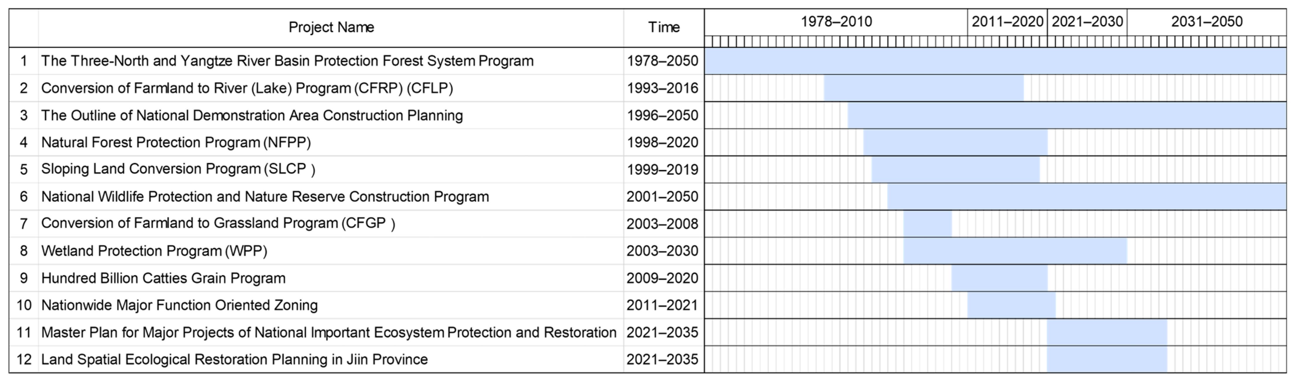
3.2. Policies-Driven Analysis

Significant work has been carried out in the fields of ecological environment protection and natural disaster prevention and control since the initiation of China’s reform and opening-up policy, as depicted in Figure 8. These efforts have resulted in notable ecological, economic, and social benefits, positioning China as a successful exemplar in global ecological governance. In November 1978, in response to the severe threat of sandstorms and soil erosion to agricultural production, China introduced the “Three-North Protection Forest Program (1978–2050)”, which pioneered large-scale ecological construction in the country. In 1995, to transform the traditional development model that resulted in resource depletion and environmental damage at a cost, and to implement sustainable development strategies, the State Environmental Protection Agency organized the formulation and publication of the “The Outline of National Demonstration Area Construction Planning (1996–2050)”. Ecological demonstration zone construction was gradually carried out nationwide, aiming to achieve a virtuous cycle of industrialization, urbanization, agricultural production, and ecological conservation [53].

A major flood disaster occurred in the Yangtze River in 1998, including the Nen River and Songhua River basins. In response, the China State Council urgently issued the “Conversion of Farmland to River (Lake) Program (1993–2016)” and the “Notice on the National Ecological and Environmental Construction Plan” [54,55], which provided specific plans for the protection of natural resources, such as natural forests, afforestation, soil and water conservation, desertification control, grassland construction, and ecological agriculture. Subsequently, the central government actively promoted the implementation of policies, such as the “Natural Forest Protection Program (2001–2050)” [56], the “Sloping Land Conversion Program (1999–2019)” [57], the “National Wildlife Protection and Nature Reserve Construction Program (2001–2050)” [58], the “Conversion of Farmland to Grass Program (2003–2008)” [59], and the “Wetland Protection Program (2003–2030)” [60].

In 2011, to implement the scientific development concept and promote the coordinated development of population, economy, resources, and the environment, the China State Council issued the “National Wide Major Function Oriented Zone (2011–2021)” [61], which provided an overall spatial layout based on the environmental carrying capacity of different regions. The northeast region is an important part of the agricultural strategic pattern of the “Seven Zones and Twenty-three Belts” and the ecological security strategic pattern of the “Two Barriers and Three Belts” [3]. In 2020, the National Development and Reform Commission and the Ministry of Natural Resources issued and implemented the “Master Plan for Major Projects of National Important Ecosystem Protection and Restoration (2021–2035)” [62], which further detailed the key projects in different ecological conservation areas, laying the institutional foundation for the ecological support of major national strategies and the sustainable development of the economy and society.

National policies constrain and guide people’s land use behaviors, exerting a significant influence on the national spatial pattern and ecological environment protection. Based on the results, it is observed that the study area has benefited from various ecological protection policies, such as the “Three-North Shelter Forestation Program (1978–2050)”, the “Natural Forest Protection Program (1998–2020)” [56], and the “Sloping Land Conversion Program (1999–2019)” [57], resulting in the protection of forest resources and a significant increase in the forest area in recent years. In addition, the policies implemented by the state for the protection of forests and wildlife reserves in the northeast region, such as “Forest Closed” [63], have led to minimal changes in the area of unused land within the study area. It can be seen that the series of ecological protection policies enacted by the state have produced positive effects on land rational utilization and the optimization of the national spatial layout.

Based on Figure 6 and Figure 8, the majority of the study area is located in the interior of the Northeast Plain, designated as the main agricultural production area in the “Seven Zones and Twenty-three Belts” and supported by the “Hundred Billion Catties Grain Program (2009–2020)”, and there is a tendency for some forest, grassland, built-up areas, and undeveloped land to be converted into farmland. However, the increase in farmland and its growth rate show a pattern of diminishing returns across three periods: 1990–2000, 2000–2010, and 2010–2020. When considering policies such as the “Conversion of Farmland to River (Lake) Program (1993–2016)”, the “Conversion of Farmland to Grassland Program (2003–2008)”, and the “Hundred Billion Catties Grain Program (2009–2020)”, it indicates that, in western Jilin, the pursuit of high productivity has led to improvements in production techniques and an increased utilization of farmland. This is projected to further decrease by 2030. The expansion of the forest land, which has been consistently increasing, demonstrates that the development in western Jilin largely aligns with the principles of sustainable development. While emphasizing production, due attention has been paid to the preservation of the ecological environment. The dynamism of the forest land has remained at a relatively high level, consistent with policies such as “The Three-North and Yangtze River Basin Protection Forest System Program (1978–2050)” and the “Natural Forest Protection Program (1998–2020)”. Against this backdrop, it is expected that the forested area will continue to increase by 2030. Under the influence of production and human activities, grassland has experienced a continuous reduction. However, supported by policies such as the “Conversion of Farmland to Grassland Program (2003–2008)”, the dynamism of grasslands has gradually decreased. Furthermore, by 2030, the grassland area is projected to exhibit a positive growth. Water, being a vulnerable component of the ecosystem, has benefited from the “Conversion of Farmland to River (Lake) Program (1993–2016)” and the “Wetland Protection Program (2003–2030)”. The water area in western Jilin has reached its minimum limit and is slowly recovering. It is predicted that, by 2030, the water area will begin to experience accelerated growth.

Taking a comprehensive perspective, policy-driven approaches play a crucial role in the spatiotemporal transformation of land use in western Jilin. Since 2020, several land use-related policies have been ongoing within the study area. According to the predicted results of this study, land use and ecological conservation in the study area still face numerous challenges. Considering the significant influence of policies on land use, it is necessary to develop more scientifically grounded policy measures that promote and incentivize the coordinated development of land use and ecological conservation.

4. Discussion

The CNN model is known for its ability to extract and learn feature representations of images effectively, making it suitable for image-processing tasks. It demonstrates a good generalization ability, computational efficiency, and prediction accuracy. However, when applied to land prediction, the CNN model often faces challenges, such as overfitting and poor interpretability. The combination of the CNN, CA, and MC models serves several purposes. Firstly, by utilizing the CNN model, we addressed the limitation of the CA model in neglecting the influence of macro-factors. Secondly, the CA and MC models help to overcome the drawbacks of the CNN model, such as slow convergence, susceptibility to local minima, and difficulty in determining network structures. Additionally, they contribute to mitigating the issues of overfitting and poor interpretability often observed in the CNN model, resulting in a higher prediction accuracy and generalization ability. In addition to the CNN, there are other neural network models commonly used, such as the multilayer perceptron (MLP) [64]. However, when coupling neural network models with the CA and MC models, the careful consideration of their network structures and processing methods is crucial to create appropriate models. For example, the MLP treats all features as equal when processing input data, disregarding spatial relationships and local features. On the other hand, the CNN utilizes convolutional kernels and pooling operations to effectively capture spatial structures and local features in the input data, thereby improving the model’s accuracy. Therefore, compared to the MLP, the CNN has stronger feature extraction capabilities and spatial awareness, making it more suitable for prediction and simulation tasks. Thus, our study can be seen as a positive attempt to use the CNN for land use prediction research.

Although we effectively predicted land use changes in western Jilin using the CNN-CA-MC model, there is still room for the in-depth interpretation of these findings. For example, a further understanding of the implications of the predicted land use changes for ecosystem services, biodiversity conservation, and climate change mitigation could provide valuable insights. However, it is important to acknowledge that land use change prediction is a complex issue. During our prediction process, inherent errors or incompleteness in the data sources can lead to inaccuracies in the model’s predictions. Additionally, errors may be introduced through parameter selection and estimation in the model, such as the transition probability matrix or the weights and biases of the neural network, which may not fully capture the complexity of land use changes. Furthermore, static parameters set based on simplified assumptions in the model may not fully capture the dynamic processes of actual land use changes. Land use changes are often influenced by stochastic factors, such as natural disasters, policy changes, or economic factors, which cannot be fully predicted or modeled, resulting in discrepancies between the predicted results and the actual conditions. Therefore, it is important to recognize the existence of these sources of errors in land use change prediction and take appropriate measures to minimize their impacts.

Despite these sources of errors, the CNN-CA-MARKOV-coupled model can still provide valuable predictions of land use changes. Linking various factors to different land use types can provide a reference and basis for land use in the future, while also offering insights into the changes in and dynamics of different land use types. However, it is essential to recognize that these findings are based on model predictions, and actual land use changes may be influenced by various factors. In future research, it is recommended to use higher quality map data and remote sensing images, ensuring data accuracy and completeness. Additionally, considering more land use-driving factors and dynamic processes as much as possible can improve the model’s performance in predicting land use changes. Multiscale modeling can be implemented to capture the CNN-CA-MC model’s performance at different scales. Introducing stochastic simulations or Monte Carlo methods to consider uncertainty can also be beneficial.

5. Conclusions

In this study, we developed an effective land use prediction method by combining the CNN model with the CA and MC models to address the limitations of each individual model and demonstrated the advantages of their integration and to predict the land use of the western Jilin. The results obtained from the coupled CNN-CA-MC model show a high prediction accuracy, exceeding 90%, indicating that the model can be effectively utilized for land use forecasting. An analysis of the policy factors related to land use was conducted to observe the significant impact on land use transformation in the short term. Further research is required to validate the accuracy of these factors. Additionally, we highlighted the suitability of the CNN model for land use prediction research, considering its strong feature extraction capabilities and spatial awareness compared to other neural network models. Despite the advantages of the CNN-CA-MC approach, the static nature of the parameters set for the CNN model in this study does not account for the dynamic nature of land use changes. Future research should strive to obtain dynamic transformation parameters to enhance the accuracy of the predictions. Furthermore, there are numerous influencing factors and threats that affect land use transformations, and incorporating more effective driving and threat factors could yield different results. Thus, a broader range of threat factors should be explored in the future.

References

1. Zhang, X.H.; Wang, Y.Q.; Qi, Y.; Wu, J.; Liao, W.J.; Shui, W.; Zhang, Y.Z.; Deng, S.H.; Peng, H.; Yu, X.Y.; et al. Evaluating the trends of China’s ecological civilization construction using a novel indicator system. J. Clean. Prod. 2016, 133, 910–923. [Google Scholar] [CrossRef]
2. Fan, J. Draft of major function oriented zoning of China. Acta Geogr. Sin. 2015, 70, 186–201. [Google Scholar] [CrossRef]
3. Fu, B. Several key points in territorial ecological restoration. Bull. Chin. Acad. Sci. 2021, 36, 64–69. [Google Scholar] [CrossRef]
4. Su, Y.Z.; Zhao, H.L.; Zhang, T.H.; Zhao, X.Y. Soil properties following cultivation and non-grazing of a semi-arid sandy grassland in northern China. Soil Tillage Res. 2004, 75, 27–36. [Google Scholar] [CrossRef]
5. Zhao, W.Z.; Xiao, H.L.; Liu, Z.M.; Li, J. Soil degradation and restoration as affected by land use change in the semiarid Bashang area, northern China. CATENA 2005, 59, 173–186. [Google Scholar] [CrossRef]
6. Piao, S.L.; Liu, Q.; Chen, A.P.; Janssens, I.A.; Fu, Y.S.; Dai, J.H.; Liu, L.L.; Lian, X.; Shen, M.G.; Zhu, X.L. Plant phenology and global climate change: Current progresses and challenges. Glob. Chang. Biol. 2019, 25, 1922–1940. [Google Scholar] [CrossRef] [PubMed]
7. Wang, X.; LESI, M.; Zhang, M. Ecosystem pattern change and its influencing factors of “two barriers and three belts”. Chin. J. Ecol. 2019, 38, 2138–2148. [Google Scholar] [CrossRef]
8. Bai, Y.; Wong, C.P.; Jiang, B.; Hughes, A.C.; Wang, M.; Wang, Q. Developing China’s Ecological Redline Policy using ecosystem services assessments for land use planning. Nat. Commun. 2018, 9, 3034. [Google Scholar] [CrossRef] [PubMed]
9. Li, C.; Wu, Y.M.; Gao, B.P.; Zheng, K.J.; Wu, Y.; Li, C. Multi-scenario simulation of ecosystem service value for optimization of land use in the Sichuan-Yunnan ecological barrier, China. Ecol. Indic. 2021, 132, 108328. [Google Scholar] [CrossRef]
10. Li, X.; Li, Y.; Wang, B.; Sun, Y.; Cui, G.; Liang, Z. Analysis of spatial-temporal variation of the saline-sodic soil in the west of Jilin Province from 1989 to 2019 and influencing factors. CATENA 2022, 217, 106492. [Google Scholar] [CrossRef]
11. Yin, L.; Wang, X.; Zhang, K.; Xiao, F.; Cheng, C.; Zhang, X. Trade-offs and synergy between ecosystem services in National Barrier Zone. Geogr. Res. 2019, 38, 2162–2172. [Google Scholar] [CrossRef]
12. Liang, J.; He, X.Y.; Zeng, G.M.; Zhong, M.H.; Gao, X.; Li, X.; Li, X.D.; Wu, H.P.; Feng, C.T.; Xing, W.L.; et al. Integrating priority areas and ecological corridors into national network for conservation planning in China. Sci. Total Environ. 2018, 626, 22–29. [Google Scholar] [CrossRef]
13. Wang, J.; Chen, Y.; Shao, X.; Zhang, Y.; Cao, Y. Land-use changes and policy dimension driving forces in China: Present, trend and future. Land Use Policy 2012, 29, 737–749. [Google Scholar] [CrossRef]
14. Zhou, B.; Xu, Y.P.; Vogt, R.D.; Lu, X.Q.; Li, X.M.; Deng, X.W.; Yue, A.; Zhu, L. Effects of Land Use Change on Phosphorus Levels in Surface Waters-a Case Study of a Watershed Strongly Influenced by Agriculture. Water Air Soil Pollut. 2016, 227, 160. [Google Scholar] [CrossRef]
15. Sun, C.Q.; Bao, Y.L.; Vandansambuu, B.; Bao, Y.H. Simulation and Prediction of Land Use/Cover Changes Based on CLUE-S and CA-Markov Models: A Case Study of a Typical Pastoral Area in Mongolia. Sustainability 2022, 14, 5707. [Google Scholar] [CrossRef]
16. Vaz, E.D.; Nijkamp, P.; Painho, M.; Caetano, M. A multi-scenario forecast of urban change: A study on urban growth in the Algarve. Landsc. Urban Plan. 2012, 104, 201–211. [Google Scholar] [CrossRef]
17. Yang, Q.S.; Li, X.; Shi, X. Cellular automata for simulating land use changes based on support vector machines. Comput. Geosci. 2008, 34, 592–602. [Google Scholar] [CrossRef]
18. Guan, D.J.; Zhao, Z.L.; Tan, J. Dynamic simulation of land use change based on logistic-CA-Markov and WLC-CA-Markov models: A case study in three gorges reservoir area of Chongqing, China. Environ. Sci. Pollut. Res. 2019, 26, 20669–20688. [Google Scholar] [CrossRef]
19. Hu, Z.Y.; Lo, C.P. Modeling urban growth in Atlanta using logistic regression. Comput. Environ. Urban Syst. 2007, 31, 667–688. [Google Scholar] [CrossRef]
20. Bununu, Y.A. Integration of Markov chain analysis and similarity-weighted instance-based machine learning algorithm (SimWeight) to simulate urban expansion. Int. J. Urban Sci. 2017, 21, 217–237. [Google Scholar] [CrossRef]
21. Saxena, A.; Jat, M.K. Capturing heterogeneous urban growth using SLEUTH model. Remote Sens. Appl. Soc. Environ. 2019, 13, 426–434. [Google Scholar] [CrossRef]
22. Karimi, F.; Sultana, S.; Babakan, A.S.; Suthaharan, S. An enhanced support vector machine model for urban expansion prediction. Comput. Environ. Urban Syst. 2019, 75, 61–75. [Google Scholar] [CrossRef]
23. Pijanowski, B.C.; Pithadia, S.; Shellito, B.A.; Alexandridis, K. Calibrating a neural network-based urban change model for two metropolitan areas of the Upper Midwest of the United States. Int. J. Geogr. Inf. Sci. 2005, 19, 197–215. [Google Scholar] [CrossRef]
24. Megahed, Y.; Cabral, P.; Silva, J.; Caetano, M. Land Cover Mapping Analysis and Urban Growth Modelling Using Remote Sensing Techniques in Greater Cairo Region-Egypt. ISPRS Int. J. Geo-Inf. 2015, 4, 1750–1769. [Google Scholar] [CrossRef]
25. Zhou, L.; Dang, X.W.; Sun, Q.K.; Wang, S.H. Multi-scenario simulation of urban land change in Shanghai by random forest and CA-Markov model. Sustain. Cities Soc. 2020, 55, 102045. [Google Scholar] [CrossRef]
26. Aburas, M.M.; Ho, Y.M.; Ramli, M.F.; Ash’aari, Z.H. Improving the capability of an integrated CA-Markov model to simulate spatio-temporal urban growth trends using an Analytical Hierarchy Process and Frequency Ratio. Int. J. Appl. Earth Obs. Geoinf. 2017, 59, 65–78. [Google Scholar] [CrossRef]
27. Jafari, M.; Majedi, H.; Monavari, S.M.; Alesheikh, A.A.; Zarkesh, M.K. Dynamic simulation of urban expansion through a CA-Markov model Case study: Hyrcanian region, Gilan, Iran. Eur. J. Remote Sens. 2016, 49, 513–529. [Google Scholar] [CrossRef]
28. Nouri, J.; Gharagozlou, A.; Arjmandi, R.; Faryadi, S.; Adl, M. Predicting Urban Land Use Changes Using a CA-Markov Model. Arab. J. Sci. Eng. 2014, 39, 5565–5573. [Google Scholar] [CrossRef]
29. Park, S.; Jeon, S.; Kim, S.; Choi, C. Prediction and comparison of urban growth by land suitability index mapping using GIS and RS in South Korea. Landsc. Urban Plan. 2011, 99, 104–114. [Google Scholar] [CrossRef]
30. Baig, M.F.; Mustafa, M.R.U.; Baig, I.; Takaijudin, H.B.; Zeshan, M.T. Assessment of Land Use Land Cover Changes and Future Predictions Using CA-ANN Simulation for Selangor, Malaysia. Water 2022, 14, 402. [Google Scholar] [CrossRef]
31. Zhang, X.R.; Zhou, J.; Song, W. Simulating Urban Sprawl in China Based on the Artificial Neural Network-Cellular Automata-Markov Model. Sustainability 2020, 12, 4341. [Google Scholar] [CrossRef]
32. Gharaibeh, A.; Shaamala, A.; Obeidat, R.; Al-Kofahi, S. Improving land-use change modeling by integrating ANN with Cellular Automata-Markov Chain model. Heliyon 2020, 6, e05092. [Google Scholar] [CrossRef]
33. Wang, X.; Li, Y.; Chu, B.; Liu, S.; Yang, D.; Luan, J. Spatiotemporal Dynamics and Driving Forces of Ecosystem Changes: A Case Study of the National Barrier Zone, China. Sustainability 2020, 12, 6680. [Google Scholar] [CrossRef]
34. Liu, J.Y.; Kuang, W.H.; Zhang, Z.X.; Xu, X.L.; Qin, Y.W.; Ning, J.; Zhou, W.C.; Zhang, S.W.; Li, R.D.; Yan, C.Z.; et al. Spatiotemporal characteristics, patterns, and causes of land-use changes in China since the late 1980s. J. Geogr. Sci. 2014, 24, 195–210. [Google Scholar] [CrossRef]
35. Guo, L.Y.; Wang, D.L.; Qiu, J.J.; Wang, L.G.; Liu, Y. Spatio-temporal patterns of land use change along the Bohai Rim in China during 1985–2005. J. Geogr. Sci. 2009, 19, 568–576. [Google Scholar] [CrossRef]
36. Liu, J.; Zhang, Z.; Xu, X.; Kuang, W.; Zhou, W.; Zhang, S.; Li, R.; Yan, C.; Yu, D.; Wu, S.; et al. Spatial patterns and driving forces of land use change in China during the early 21st century. J. Geog. Sci. 2010, 20, 483–494. [Google Scholar] [CrossRef]
37. Ning, J.; Liu, J.Y.; Kuang, W.H.; Xu, X.L.; Zhang, S.W.; Yan, C.Z.; Li, R.D.; Wu, S.X.; Hu, Y.F.; Du, G.M.; et al. Spatiotemporal patterns and characteristics of land-use change in China during 2010–2015. J. Geogr. Sci. 2018, 28, 547–562. [Google Scholar] [CrossRef]
38. Eastman, J.R. IDRISI Taiga Guide to GIS and Image Processing; Clark Labs Clark University: Worcester, MA, USA, 2009. [Google Scholar]
39. Eastman, J.R. IDRISI Kilimanjaro: Guide to GIS and Image Processing; Clark Labs Clark University: Worcester, MA, USA, 2003. [Google Scholar]
40. Eastman, J.R. IDRISI Andes Manual; Clark Labs, Clark University: Worcester, MA, USA, 2006. [Google Scholar]
41. Gu, J.X.; Wang, Z.H.; Kuen, J.; Ma, L.Y.; Shahroudy, A.; Shuai, B.; Liu, T.; Wang, X.X.; Wang, G.; Cai, J.F.; et al. Recent advances in convolutional neural networks. Pattern Recognit. 2018, 77, 354–377. [Google Scholar] [CrossRef]
42. Kattenborn, T.; Leitloff, J.; Schiefer, F.; Hinz, S. Review on Convolutional Neural Networks (CNN) in vegetation remote sensing. ISPRS J. Photogramm. Remote Sens. 2021, 173, 24–49. [Google Scholar] [CrossRef]
43. Oostwal, E.; Straat, M.; Biehl, M. Hidden unit specialization in layered neural networks: ReLU vs. sigmoidal activation. Phys. A 2021, 564, 125517. [Google Scholar] [CrossRef]
44. Getu, K.; Bhat, H.G. Dynamic simulation of urban growth and land use change using an integrated cellular automaton and markov chain models: A case of Bahir Dar city, Ethiopia. Arab. J. Geosci. 2022, 15, 1049. [Google Scholar] [CrossRef]
45. Muller, M.R.; Middleton, J. A Markov model of land-use change dynamics in the Niagara Region, Ontario, Canada. Landscape Ecol. 1994, 9, 151–157. [Google Scholar] [CrossRef]
46. Yang, X.; Zheng, X.Q.; Lv, L.N. A spatiotemporal model of land use change based on ant colony optimization, Markov chain and cellular automata. Ecol. Model. 2012, 233, 11–19. [Google Scholar] [CrossRef]
47. Batty, M.; Xie, Y.; Sun, Z. Modeling urban dynamics through GIS-based cellular automata. Comput. Environ. Urban Syst. 1999, 23, 205–233. [Google Scholar] [CrossRef]
48. Peterson, L.K.; Bergen, K.M.; Brown, D.G.; Vashchuk, L.; Blam, Y. Forested land-cover patterns and trends over changing forest management eras in the Siberian Baikal region. For. Ecol. Manag. 2009, 257, 911–922. [Google Scholar] [CrossRef]
49. Prieto-Amparán, J.A.; Pinedo-Alvarez, A.; Villarreal-Guerrero, F.; Pinedo-Alvarez, C.; Morales-Nieto, C.; Manjarrez-Domínguez, C. Past and Future Spatial Growth Dynamics of Chihuahua City, Mexico: Pressures for Land Use. ISPRS Int. J. Geo-Inf. 2016, 5, 235. [Google Scholar] [CrossRef]
50. Zadbagher, E.; Becek, K.; Berberoglu, S. Modeling land use/land cover change using remote sensing and geographic information systems: Case study of the Seyhan Basin, Turkey. Environ. Monit. Assess. 2018, 190, 494. [Google Scholar] [CrossRef]
51. Dai, L.M.; Zhao, W.; Shao, G.F.; Lewis, B.J.; Yu, D.P.; Zhou, L.; Zhou, W.M. The progress and challenges in sustainable forestry development in China. Int. J. Sustain. Dev. World Ecol. 2013, 20, 394–403. [Google Scholar] [CrossRef]
52. Jin, X.B.; Shao, Y.; Zhang, Z.H.; Resler, L.M.; Campbell, J.B.; Chen, G.; Zhou, Y.K. The evaluation of land consolidation policy in improving agricultural productivity in China. Sci. Rep. 2017, 7. [Google Scholar] [CrossRef]
53. Huang, P.; Westman, L. Policy experimentation in the construction of ecological civilisation in China. In Handbook on Adaptive Governance; Edward Elgar Publishing: Cheltenham, UK, 2023; pp. 176–191. [Google Scholar]
54. Ma, S.; Qiao, Y.P.; Jiang, J.; Wang, L.J.; Zhang, J.C. Incorporating the implementation intensity of returning farmland to lakes into policymaking and ecosystem management: A case study of the Jianghuai Ecological Economic Zone, China. J. Clean. Prod. 2021, 306, 127284. [Google Scholar] [CrossRef]
55. Yu, G.R.; Yang, M.; Chen, Z.; Zhang, L.M. Technical approach and strategic plan for large-scale ecological and environmental governance and national ecological security pattern construction. J. Appl. Ecol. 2021, 34, 1141–1153. [Google Scholar] [CrossRef]
56. Ren, G.P.; Young, S.S.; Wang, L.; Wang, W.; Long, Y.C.; Wu, R.D.; Li, J.S.; Zhu, J.G.; Yu, D.W. Effectiveness of China’s National Forest Protection Program and nature reserves. Conserv. Biol. 2015, 29, 1368–1377. [Google Scholar] [CrossRef]
57. Lu, G.; Yin, R.S. Evaluating the Evaluated Socioeconomic Impacts of China’s Sloping Land Conversion Program. Ecol. Econ. 2020, 177, 106785. [Google Scholar] [CrossRef]
58. Liu, W.; McGowan, P.J.K.; Xu, J.; Zhang, Z. A review and assessment of nature reserve policy in China: Advances, challenges and opportunities. Oryx 2012, 46, 554–562. [Google Scholar] [CrossRef]
59. Li, S.; Li, M. The development process, current situation and prospects of the conversion of farmland to forests and grasses project in China. J. Resour. Ecol. 2022, 13, 120–128. [Google Scholar] [CrossRef]
60. Shi, M.; Qi, J.; Yin, R. Has China’s Natural Forest Protection Program Protected Forests?—Heilongjiang’s Experience. Forests 2016, 7, 218. [Google Scholar] [CrossRef]
61. Jie, F.; Anjun, T.; Qing, R. On the historical background, scientific intentions, goal orientation, and policy framework of major function-oriented zone planning in China. J. Resour. Ecol. 2021, 1, 289–299. [Google Scholar] [CrossRef]
62. Cui, W.H.; Liu, J.G.; Jia, J.L.; Wang, P.F. Terrestrial ecological restoration in China: Identifying advances and gaps. Environ. Sci. Eur. 2021, 33, 123. [Google Scholar] [CrossRef]
63. Deng, X.Z.; Jiang, Q.O.; Zhan, J.Y.; He, S.J.; Lin, Y.Z. Simulation on the dynamics of forest area changes in Northeast China. J. Geogr. Sci. 2010, 20, 495–509. [Google Scholar] [CrossRef]
64. Taud, H.; Mas, J.F. Multilayer Perceptron (MLP). In Geomatic Approaches for Modeling Land Change Scenarios; Camacho Olmedo, M.T., Paegelow, M., Mas, J.F., Escobar, F., Eds.; Springer International Publishing: Cham, Switzerland, 2018; pp. 451–455. [Google Scholar]
Figure 1. The location of the study area.
Atmosphere 15 00288 g001
Figure 2. The framework of the CNN-CA-CN model.
Atmosphere 15 00288 g002
Figure 3. The details of the CNN model. (a) The model architecture of the CNN model. (b) The training of the CNN model.
Atmosphere 15 00288 g003aAtmosphere 15 00288 g003b
Figure 4. Land use in 2020. (a) Predicted. (b) Actual. (c) Predicted vs. actual land use match/mismatch map.
Atmosphere 15 00288 g004
Figure 5. The projected land use in 2030.
Atmosphere 15 00288 g005
Figure 6. Comparison of the land use area. (a) Actual and predicted land use areas. (b) Gains and losses in the period of 2020–2030 (% of area).
Atmosphere 15 00288 g006aAtmosphere 15 00288 g006b
Figure 7. Gains and losses of land use between 2020 and 2030. (a) Farmland. (b) Forest. (c) Grassland. (d) Water. (e) Built-up areas. (f) Undeveloped land.
Atmosphere 15 00288 g007aAtmosphere 15 00288 g007b
Figure 8. The main policies that are related to the study area.
Atmosphere 15 00288 g008