Abstract
As numerical weather forecasting advances, there is a growing demand for higher-quality atmospheric data. Hyperspectral instruments can capture more atmospheric information and increase vertical resolution, but there has been limited research into retrieval algorithms for obtaining hyperspectral microwaves in the future. This study proposes an atmospheric temperature profile detection algorithm based on Convolutional Neural Networks (CNN) and Local Attention Mechanisms for local feature extraction, applied to hyperspectral microwave sensors. The study utilizes the method of information entropy to extract more effective channels in the vicinities of 60 GHz, 118 GHz, and 425 GHz. The algorithm uses the brightness temperature as the input of the network. The algorithm addresses common issues encountered in conventional networks, such as overfitting, gradient explosion, and gradient vanishing. Additionally, this method isolates the three oxygen-sensitive frequency bands for modularized local feature extraction training, thereby avoiding abrupt changes in brightness temperature between adjacent frequency bands. More importantly, the algorithm considers the correlation between multiple channels and information redundancy, focusing on variations in local information. This enhances the effectiveness of hyperspectral microwave channel information extraction. We simulated the brightness temperatures of the selected channels through ARTS and divided them into training, validation, and test sets. The retrieval capability of the proposed method is validated on a test dataset, achieving a root mean square error of 1.46 K and a mean absolute error of 1.4 K for temperature profile. Detailed comparisons are also made between this method and other commonly used networks for atmospheric retrieval. The results demonstrate that the proposed method significantly improves the accuracy of temperature profile retrieval, particularly in capturing fine details, and is more adaptable to complex environments. The model also exhibits scalability, extending from one-dimensional (pressure level) to three-dimensional space. The error for each pressure level is controlled within 0.7 K and the average error is within 0.4 K, demonstrating effectiveness across different scales with impressive results. The computational efficiency and accuracy have both been improved when handling a large amount of radiation data.
1. Introduction
Temperature profiles play a crucial role in various fields such as atmospheric stability analysis, atmospheric boundary layer studies, climate change research, and weather forecasting [1,2,3,4,5]. Therefore, research on and the development of instruments for temperature profile detection, numerical calculations, and parameter retrieval are of great significance to the advancement of meteorology [6,7,8].
Hyperspectral observations can provide more atmospheric information. Currently, infrared hyperspectral technology is relatively mature for remote sensing, while microwave radiometers typically use a limited number of channels. A. E. Lipton et al. [9] proposed a method in 2003 to establish a suitable combination of center frequencies and bandwidths for atmospheric microwave detection. In 2011, W. J. Blackwell et al. [10] introduced the concept of hyperspectral microwaves, and then, D. Liu [11] and his team developed ground-based hyperspectral microwave radiometer products, which yielded excellent results. Subsequently, many scholars have conducted further research. For example, J.-F. Mahfouf et al. [12] optimized channel selection using the atmospheric database of the European Centre for Medium-Range Weather Forecasts (ECMWF). F. Aires et al. [13] investigated the advantages of satellite hyperspectral microwave sensors (HYMS) in inverting atmospheric temperature and humidity profiles under the background of numerical weather prediction (NWP). Recently, Yanmeng Bi [14] and his colleagues found that sampling thinner absorption lines at higher spectral resolutions not only allows for a higher vertical resolution but also helps in mitigating radio frequency interference. Therefore, research into satellite-based hyperspectral microwaves has a promising and clear prospect, enabling more effective characterization of atmospheric vertical distribution features.
Regarding the retrieval algorithm for secondary data from remote sensing instruments, several methods have been applied, including the eigenvector method [15], the optimal estimation method [16], the physical iteration method [17], and the more recent popular neural network method with better non-linear fitting capabilities [18]. Backpropagation neural network algorithms (BPNN) and their variants are widely used, with some models having multiple hidden layers to improve model generalization [19,20]. Additionally, some scholars have made improvements to these models by incorporating batch normalization layers and dropout layers to enhance model robustness [21,22]. Introducing a one-dimensional CNN model for training on one-dimensional data requires a novel approach. However, a detailed exploration of this method is lacking [23].
Despite many scholars having explored the prospects of hyperspectral microwave applications and there being many retrieval methods, no one has delved deep into the retrieval methods for hyperspectral microwaves. We propose an approach that takes into consideration the characteristics of hyperspectral data to address this issue. Specifically, we introduce a method for local feature extraction based on a CNN and attention mechanisms. This method utilizes convolutional kernels and pooling layers in high-density frequency channels, coupled with a local attention adaptation. It captures local information (referring to the peak centers of the weight functions) while suppressing unimportant information (referring to the mutual interference between channels). The method is validated and discussed by simulating brightness temperatures from the Seebor Version 5.0 (SeeborV5) global atmospheric profile data and Global/Regional Assimilation and Prediction System (GRAPES) database using the Atmospheric Radiative Transfer Simulator (ARTS). Simultaneously, the perturbation matrix (Jacobian matrix) was calculated. The information content method was then employed to extract channels with more information content and the concept of cumulative information was introduced. Furthermore, a detailed comparison with commonly used deep learning models for atmospheric profile retrieval is performed. The model also demonstrates adaptability across different scales, with its advantages in local information extraction making it suitable for temperature retrieval in three-dimensional space. In the final analysis, the performance of this model is validated using GRAPES data.
2. Data and Preprocessing
2.1. SeeborV5 Atmospheric Profiles Database
The training data were sourced from the Cooperative Institute for Meteorological Satellite Studies (CIMSS) global atmospheric profile database, SeeborV5. They include 15,704 temperature profiles and other atmospheric profiles under clear sky conditions. These data are sourced from climate monitoring instruments or sensors such as NOAA-88. For consistency and ease of subsequent brightness temperature simulation and comparison, we integrated the data to obtain 97 pressure levels with the same distribution. To enhance computational speed and validate the effectiveness of the method, we shuffled the dataset and randomly extracted 4440 profiles of pressure measurements from the Asian region, as shown in Figure 1. Subsequently, we partitioned the dataset into training, validation, and test sets, with proportions of 80%, 15%, and 5%, respectively. However, it should be noted that these data are not exact. Interpolation methods were applied when extending the pressure levels, leading to uncertain errors.
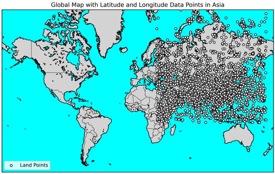
Figure 1.
SeeborV5 data distribution in the Asian region.
2.2. GRAPES Database
GRAPES (Global/Regional Assimilation and Prediction System) is an atmospheric numerical model system initiated by the China Meteorological Administration (CMA). The system aims to provide high-resolution and high-quality atmospheric observational data for numerical weather and climate predictions. GRAPES integrates global and regional observational data, employing advanced numerical models and data assimilation techniques to enhance the simulation and predictive capabilities of atmospheric and Earth-surface processes. The system encompasses meteorological elements at the global, regional, and multiple vertical height levels. Through the real-time assimilation of observational data, the model output aligns more closely with actual observed conditions. In this study, we selected the 40-layer pressure profiles for the Asian region in July 2022, with a spatial resolution of 0.5° in latitude and longitude. The GRAPES data grid has a high resolution and requires significant computational power. Only a portion of the data (60–150° E) were selected for network training. Figure 2 depicts the 3D temperature map for 1 July 2022, at 0000 UTC. The dataset comprises a total of 1302 samples for the month of July. The selection ratios for the training set, validation set, and test set are consistent with the aforementioned proportions. The vertical resolution is within 1–3 km, with an accuracy of 1 K.
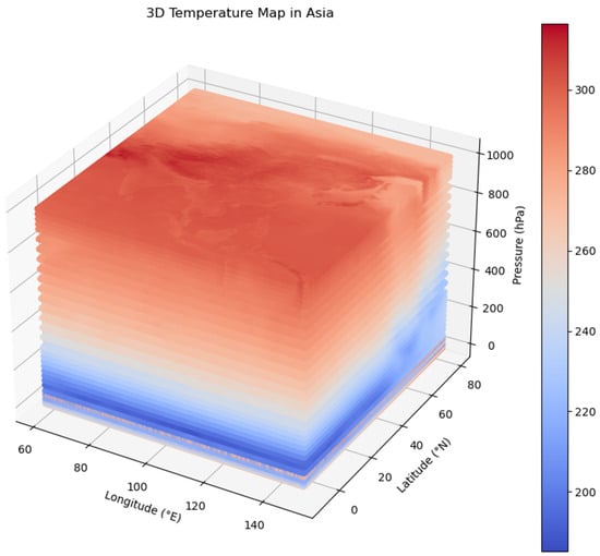
Figure 2.
GRAPS temperature gird data distribution at 60–150° E, 10–80° N.
2.3. The Simulation of Brightness Temperature Data
In this study, the Atmospheric Radiative Transfer Simulator (ARTS) was used to simulate a set of brightness temperature values near the oxygen absorption peak. We imported HITRAN2020 spectral absorption coefficient data into the ARTS transmission model to calculate Collision-induced absorption (CIA). The calculations involved the use of ARTS’ unique agenda for line-by-line numerical computations, accessing various coefficient files. The PWR-98 mode was employed when computing oxygen and water vapor. The model also allows for sensor simulation, requiring configuration of sensor responses, line of sight, altitude, azimuth, and other parameters.
Furthermore, ARTS is capable of calculating Jacobian matrices under non-scattering conditions to describe atmospheric disturbances from relevant molecules [24]. For this study, we selected a satellite orbit height of 450 km, a nadir viewing angle of 0–180°, and operational frequencies near 60 GHz, 118 GHz, and 425 GHz. We referenced the specifications of other instruments (HYMS, ATMS, and FY-4) to configure the simulation’s sensor parameters. Table 1 summarizes the main parameters.

Table 1.
ARTS simulation hyperspectral band parameter settings.
Before putting brightness temperature data into the model, each data item was normalized using the Z-score method [21]. The expressions are as follows.
2.4. Calculation of Cumulative Information Content
Currently, many scholars and researchers utilize the concept of information entropy to optimize the channels of radiometers, aiming to reduce design costs and instrument weight. In 2000, Rodgers introduced information theory into the optimization of high-spectral-resolution instruments by calculating the information entropy H(x) for each channel using the background error covariance, and observing the error covariance and the Jacobian matrix [25]. Later, J.-F. Mahfouf et al. [12] and others conducted detailed information content calculations for channels sensitive to temperature and water vapor using ECMWF data. They concluded that 137 channels, which account for 90% of the information content, are sufficient to achieve good results. Although this paper does not focus on channel selection, it still considers the 90% information content as the criterion for channel selection. Because the data itself carries inherent errors, the selected channels may only be applicable to this specific dataset. Below is a brief introduction to the information content calculation method used in this paper. The probability density function of the atmospheric state before measurement is denoted as P(x), and the probability density function of the atmospheric state after measurement is denoted as P(x|y). Here, x represents the atmospheric state variables, and y represents the observation values (brightness temperature). The obtained information content is calculated as follows:
To simplify the calculation, we assume that x follows a Gaussian distribution with a background error covariance matrix (calculated based on the sample database using the NMC method). The posterior covariance matrix is denoted as , and the observation error covariance matrix is denoted as (set as 0.2 K2 in this study). The estimation of is performed using a Bayesian model in its quadratic form.
where K represents weighting functions. In this paper, the method of channel-by-channel selection is used, and finally, the single-channel information content is simplified as follows:
where r represents:
In reality, although the weighting function for each channel is fixed, the perturbation of temperature profiles varies due to different atmospheric conditions influenced by various molecular absorption characteristics. Consequently, the actual peak values of the weighting functions can also change. Therefore, it may be necessary to adjust the frequency channels for different atmospheric conditions.
In Equation (7), we consider the summation of information entropy associated with varying Jacobian matrices, and then we obtain cumulative information. (If the data are time-dependent, this method can also be employed). This is because a geostationary satellite radiometer can continuously observe atmospheric physical information in a specific area over an extended period. The accumulated information content for observing a specific atmospheric physical feature over a continuous period is considered as a criterion for channel selection. The retrieved brightness temperature data from the profile forward modeling are treated as continuous observations from a satellite microwave radiometer. Figure 3 shows the selected 268 channels. The bandwidth is 50 MHz. Figure 4 shows the simulated brightness temperature of selected channel for one sample.
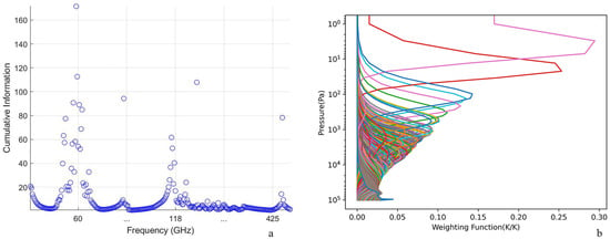
Figure 3.
(a) By employing the cumulative information content method, we have selected 268 temperature profile retrieval channels distributed around 60 GHz, 118 GHz, and 425 GHz. (b) Channel weighting function we selected.
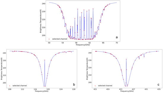
Figure 4.
Through the method of cumulative information content, 268 oxygen-sensitive channels were selected. (a) shows 155 channels in the range of 50–60 GHz, (b) shows 59 channels in the range of 108–128 GHz, and (c) shows 54 channels in the range of 415–435 GHz.
3. Method
3.1. CNN-LAA
This is a parallel structure composed of CNN, LAA, and fully connected layers. Based on the characteristics of the weight function and the Jacobian perturbation matrix, the channels in microwave detection should aim to minimize correlation. However, in between narrow peaks, the brightness temperature contributions should influence each other, leading to certain correlations. Therefore, we utilized convolution kernels (similar to filters) to integrate information from adjacent channels, capturing the brightness temperature variations and local features in a specific frequency band. The pooling layer extracts important information from local features while suppressing unimportant details, thus reducing information redundancy. Through the convolution and pooling layers, we extract the contributions of adjacent channels to the brightness temperature, effectively reducing redundancy. Therefore, selecting appropriate sizes for the convolution kernels and pooling layers is crucial. Figure 5 shows the process of convolution kernel computation. Each convolution operation integrates the brightness temperature values of adjacent frequency channels to obtain a new value, representing the overall information for that frequency range. Since the stride is smaller than the width of the kernel, it helps prevent the loss of information features.
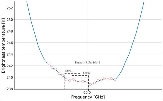
Figure 5.
We selected a sample with smooth brightness temperature variations near 60 GHz as an example for convolution kernel computation. In reality, channel frequencies are more densely spaced, but for the purpose of illustration, we chose a bandwidth of 50 MHz, a kernel size of 5, and a stride of 2. The window represents the region for each computation.
Using the aforementioned method to evaluate information content, we obtained a total of 268 high-information channels. In Figure 6, our proposed approach is based on the convolution, comprising two convolution layers, two pooling layers, dropout layers, and two fully connected layers. The 268 frequency channels are treated as input features in our method. Deeper networks with smaller convolutional kernels often yield better training results than shallower networks with larger kernels. The first convolution layer contains six channels (each channel is the result of applying different convolution kernels), each with a length of five. We applied the Relu activation function to the output of each layer (the activation function layer is omitted in the diagram). The length was then reduced by a pooling layer with a size of 2. The second convolution layer has ten channels, each with a kernel size of six, and the second pooling layer has a size of 2. The data then enter two fully connected layers, enhancing the model’s ability to handle non-linear relationships. The dropout layer (with a dropout rate of 0.1) is employed to prevent overfitting, limit the model’s flexibility, and improve robustness.
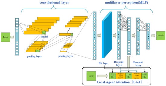
Figure 6.
Schematic of the CNN-LAA. Green color represents the input and output data. Blue color represents the layers.
During the model building and training process, we compared the effects of max pooling and average pooling layers. Both yielded similar results in terms of inversion. However, utilizing the average pooling layer considered the stacking effect of weight functions between adjacent channels, resulting in better handling of details. On the other hand, using the max pooling layer highlighted the response of sensitive channels but weakened the effect of high-spectral channels. However, without using pooling layers, the inversion effect degraded into that of a BPNN. With increased network depth, overfitting occurred on the validation set, making it unstable. Subsequently, we incorporated a parallel Attention mechanism, where the weights of key-sensitive channels were emphasized, compensating for the smoothing effect on sensitive channels. Therefore, we chose the average pooling layer.
It is important to note that the convolution will be calculated over adjacent data. However, the impact of different frequency bands on the retrieval result might not be the same, as each frequency band provides different information, which affects the temperature retrieval at corresponding altitudes differently. Bayesian’s residual network improves classified tasks performance [26]. Inspired by this, we incorporated a Local Agent Attention (LAA). In the first linear layer, we incorporate information from the input layer. This linear layer has more neurons than the 268 originally present. Consequently, we split the data from the 60 GHz, 118 GHz, and 425 GHz frequency channels into three parts, filling the adjacent parts with the output from the first dropout layer to match the dimensions of the first linear layer. We then used the and recorded by the Batch Normalization (BN) layers [27] corresponding to each frequency channel as weights and biases added to the three parts of the input data. The inclusion of this module resulted in a 15.7% improvement in performance. Therefore, adding input information can mitigate information crosstalk between different frequency bands. The added input data are:
We introduced a local attention mechanism and a block model, where the model focuses on a small portion of the input information in one step. The model structure of LAA is illustrated in Figure 7, using brightness temperature data from the 50 GHz to 70 GHz frequency range as an example. The local window size of the model is set to 3, with an additional patch added at both ends for padding, ensuring consistency in the dimensions between the output and input data. To simplify, we will abbreviate the model output as:
where represent the query, key, and value matrices, is the number of layers, and is the dimension. comes from a pooling operation applied to . And denotes Softmax attention operations.

Figure 7.
Schematic of the LAA layer. (a) illustrates a local attention mechanism, taking the 50–70 GHz frequency range as an example with a sliding window size of 3. (b) depicts the architecture of the Agent Attention model.
The input data contain brightness temperature values for each channel (possibly one-dimensional and three-dimensional data, with the three-dimensional data containing latitude and longitude). Each window slide includes brightness temperature values for three channels, thereby obtaining an input set.
where I represents the input data, and i represents the number of channels in three bands.
We introduced a new matrix A between Q and K. Initially, it replaces K, aggregating all the information from V and Q, undergoing a softmax attention operation. Subsequently, it serves as the new V returned to K for a second softmax attention operation. This agent possesses a hyperparameter n to maintain modeling capability and reduce computational complexity. To compensate for the lack of feature diversity, we incorporated the DWC module to enhance the model’s feature diversity. However, this is unnecessary for one-dimensional features.
The output of three frequency bands is concatenated with the output of the previous level. Equation (8) can be transformed into:
This approach selectively attends to a narrow window of the preceding and succeeding data, addressing three issues:
- The local attention mechanism reduces parameters, leading to faster training compared to soft attention, while maintaining differentiability in the data. The distinctive feature of Agent Attention (AA) [28], as compared to other attention mechanisms, lies in the introduction of the agent matrix, leading to a significant reduction in computational complexity. The algorithm complexity is O(Nnd).
- It is easier to train compared to hard attention, achieving a better balance between computational efficiency and model performance.
- It is more conducive to parallelization, as each step only needs to focus on a small local window, contributing to improved training and inference efficiency. During training, we observed that aligning the attention mechanism with the convolutional module’s kernel size yielded the best results, highlighting the significance of input data processing in the training process.
3.2. Other Retrieval Methods
A 1D-CNN (One-Dimensional Convolutional Neural Network) is typically used to handle sequential data with positional relationships. James [23] and his colleagues developed a deep neural network for evaluating future satellite-based hyperspectral microwave sensor designs. They utilized the predictive performance of these networks as an indicator of the overall suitability of the instrument, addressing the issue of optimal channel selection. Multiple 1D-CNN modules were applied in the process, providing a beneficial approach to solving the optimal channel selection problem. The study also found that the model is particularly well-suited for complex simulated instruments, exhibiting high accuracy.
BPNN (Backpropagation Neural Network) is a neural network algorithm and currently one of the most common methods used in retrieval algorithms. It can learn and continuously adjusts the model’s parameters with historical data, providing good non-linear fitting capabilities. X. Yan et al. [21] applied BPNN to the retrieval of temperature and relative humidity from ground-based microwave radiometers and made different improvements to the model. Similarly, many scholars used BPNN in their research on hyperspectral microwave channel selection. Comparing it with the method proposed in this paper would be meaningful.
XGBoost (eXtreme Gradient Boosting) is an ensemble learning algorithm that can be considered as a further optimization and extension of decision trees and random forests. It inherits the structure of decision trees and the ensemble algorithm ideas from random forests. In order to improve the accuracy of air quality predictions, Angel Anwagise [29] and his team developed a predictive model based on the XGBoost algorithm. They conducted experiments using a dataset collected from Kaggle. During the model’s development, they took into account the levels of pollutants such as lead, sulfur dioxide, and nitrogen dioxide, treating these data as a time series, and used them to train the model for predicting and evaluating air quality index.
SVM (Support Vector Machine) holds a crucial position in machine learning and is a powerful and versatile model, particularly representative in regression algorithms. It is frequently used in meteorology for inverting atmospheric parameters and classifying targets. For instance, A. Gong et al. [30] successfully employed SVM to perform nonlinear retrieval of near-surface air temperature using satellite remote sensing data and other information.
4. Results
4.1. Comparison of Retrieval Performance with Other Methods
To validate the performance of the proposed CNN-LAA model in this paper, we compared it with other commonly used methods for atmospheric profile retrieval and meteorological data monitoring. Table 2 provides a detailed comparison of the root mean square error (RMSE), mean absolute error (MAE), and coefficient of determination (R2) obtained from each method’s retrievals. We adapted the methods described in the literature above for use in an improved model tailored for satellite-based hyperspectral microwave applications. For the temperature profile retrieval, the CNN-LAA method achieved the best results with RMSE and MAE of 1.46 K and 1.40 K, respectively. It exhibited good fitting performance. Following closely was the BPNN method.

Table 2.
Comparison of retrieval performance with different methods.
The RMSE and MAE used here refers to the overall root mean square error as follows [31].
In terms of temperature retrieval, there is not a significant difference in accuracy between BPNN and CNN methods. However, it is worth noting that the CNN-LAA method performs better in capturing details. As shown in Figure 8a (where the temperature variation is smooth), there is an inversion layer (troposphere) at around 12 km (approximately 15,000 pa), and after breaking through the tropopause, the temperature gradually increases, entering the stratosphere, and then the temperature gradually decreases after crossing the stratopause. In the upper atmosphere, the electromagnetic energy of particles’ absorption and radiation experiences less atmospheric attenuation, contributing significantly to the radiance temperature of satellite-based microwave radiometers (the magnitude of contribution corresponds to the peak of the weighting function in frequency channels). Hence, at this altitude, frequency channels with strong sensitivity to oxygen molecules contain a substantial amount of information. The CNN’s convolutional layers and pooling layers can extract local features effectively. When temperature fluctuations occur, traditional BPNN’s retrieval results may not be sensitive to temperature changes, leading to the representation of only the overall trend. In contrast, CNN-LAA can capture variations in brightness temperature values in certain sensitive and narrow spectral channels, which effectively improves the model’s generalization ability. Most temperature profiles follow a smooth curve depicting the variation of temperature with altitude. Traditional deep learning methods can achieve satisfactory retrieval results based on such profiles. We selected a temperature profile situated near the subpolar low-pressure zone. Apart from the troposphere, both the stratosphere and mesosphere exhibit numerous small peaks. Details (retrieval bias of temperature) are shown in Figure 8b. We can see that, in an unstable atmospheric environment, the CNN-LAA method exhibits better robustness, which is conducive to understanding atmospheric patterns and improving meteorological forecasting. The error for each layer remains near the 0 K line, with the majority staying within 2 K.
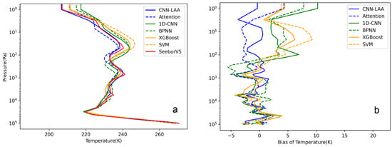
Figure 8.
(a) Comparison of temperature profiles generated by CNN1d, BPNN, XGBoost, and SVM retrieval methods for a special sample (63°68′ E,70°54′ N) in SeeborV5. In this sample, the data exhibit significant fluctuations or oscillations, indicating high volatility. (b) Retrieval bias of temperature by different methods from special sample in (a).
4.2. Bias of Temperature with Pressure
Each sample has 97 levels, and Figure 9 presents a comparison of temperature deviations in temperature profiles generated by six different deep learning retrieval methods at various vertical pressures, with a plot for every five layers. In the pressure layers above 1100 Pa, all methods exhibit relatively small temperature deviations. However, the retrieval performance in the high-altitude atmosphere is generally unsatisfactory due to two main reasons: firstly, there are very few frequency channels with weight function peaks located in the high-altitude atmosphere; secondly, the global atmospheric profile database under clear-sky conditions has a wide distribution, with significant variations in temperature profiles across different times, terrains, and climatic conditions, leading to “jumps” and uncertainties in the high-altitude atmospheric data. These two factors make it challenging for the information from the high-altitude atmosphere to be reflected in the brightness temperature values. It can be observed that the CNN still maintained a relatively high level of accuracy in such cases, which also provides new insights for the retrieval of upper atmospheric information. The results show that the CNN-LAA method performs well in the range of 10 hPa to 70 hPa, with errors controlled at around 1 K. It demonstrates good stability in the overall profile retrieval performance. Following closely are the 1D-CNN and Attention networks, with similar performances, possibly due to their similar model architectures, both possessing characteristics of local feature extraction and computation. BPNN also performs well at a mid-level pressure.
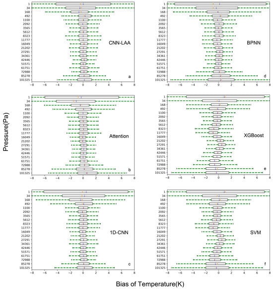
Figure 9.
The figure displays the temperature retrieval biases on the test set. Subfigures (a–f) shows the retrieval bias of temperature (the retrieval temperature minus testdata temperature) generated by six different deep learning retrieval methods. The yellow solid line represents the median, while the blue dashed line represents the mean.
From the image, it can be observed that the retrieval performance of SVM and XGBOOST methods seems to be relatively poor. In the atmospheric layers with higher and lower pressures, the retrieval results are not ideal. This aligns with the physical interpretation of frequency channel weighting functions, as microwave radiometers on satellites mainly receive radiation from the middle atmospheric layer, where the gas molecule content is higher, and the radiation capability is limited. The radiation from the lower atmospheric layer also undergoes losses during the path, impacting the retrieval results.
Regarding the retrieval performance in the middle atmospheric layer, the CNN-LAA, Attention, 1D-CNN, and BPNN methods show good results, with temperature bias primarily concentrated within ±1 K, while XGBoost and SVM exhibit relatively larger fluctuations. For the atmospheric top and bottom layers, CNN-LAA achieves the best performance.
4.3. The Retrieval Performance of CNN-LAA in Three-Dimensional Space
The three-dimensional CNN-LAA is capable of inverting observed brightness temperatures within a certain spatial range. It takes into account the spatial continuity and correlation of weather systems and atmospheric parameter distributions. The key difference from the one-dimensional CNN-LAA lies in the adjustment of the convolutional layer’s depth, which is increased to five convolutional layers. This deepening of the network makes it suitable for more complex relationship models, enhancing its generalization capabilities.
In the case of three-dimensional space, the model fully utilizes the advantages of convolutional networks in handling high-dimensional data. Simultaneously, it leverages the local attention mechanism to process local data effectively. The atmospheric temperature in the training sample dataset is based on GRAPES reanalysis data, divided into 40 layers vertically from 1000 hPa to 0.01 hPa. Taking the data from 2 July 2022, 0000 UTC as an example, the size of a single atmospheric temperature profile sample is 360 × 360 × 40 (Figure 10, using 1000 hPa temperature as an example). Due to the large data size of a single sample, exceeding the physical memory of computers, each sample is processed into 144 smaller samples of size 30 × 30 × 40. The brightness temperature images of frequency channels should also be segmented into the same size, with each sample having dimensions of 30 × 30 × 268.
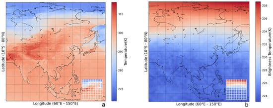
Figure 10.
(a) depicts the gridded temperature over the Asian region at 1000 hPa, segmented into 144, 30 × 30 images. Meanwhile, in figure (b), the brightness temperature image of the 58.50 GHz frequency channel is presented, also divided into 144, 30 × 30 images.
Figure 11 illustrates a scatter plot comparing the retrieved temperatures by the CNN-LAA with the test sample temperatures for the region in July 2022. The correlation coefficient between the CNN-LAA retrieved temperatures and the test sample temperatures is 0.9958, indicating a high level of correlation. The retrieved temperatures show an overall bias of 0.42 K compared to the test samples, with an RMSE averaged over the entire layer at 0.4 K. The temperature retrieved by the inversion shows a distribution on both sides of the 0.4 K line, roughly corresponding to the pressure range from 1000 hPa to 10 hPa. Around the altitudes of 200 hPa and 70 hPa, where the height of the atmospheric layers is concentrated, the fluctuation of the temperature profile retrieved by the inversion remains relatively small. The highest accuracy in temperature retrieval is observed in the middle layers of the troposphere (7–20 hPa), with temperature root mean square error (RMSE) hovering around 0.2 K. The difference between MAE and RMSE is within 0.1 K.
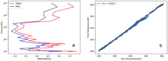
Figure 11.
(a) illustrates the RMSE and MAE of temperature retrieval at different pressure levels. (b) shows the correlation coefficient between the validation set and the predicted data.
5. Discussion
With the advancement of computers and improved instrument precision, we now have access to abundant and highly accurate historical data, providing strong support for neural network models in atmospheric profile retrieval. In the context of temperature profile retrieval, researchers often used single-layer or multi-layer feedback neural networks. Neural network methods primarily rely on training and adjusting network parameters to perform nonlinear function fitting. However, attention needs to be paid to the feature distribution of training samples, as well as the structures of input and output data, to select an appropriate model. The CNN-LAA method proposed in this paper differs from traditional algorithms as it considers the features of both inputs and outputs. Hyperspectral microwave data possess multiple frequency channels, which are constructed by establishing a large number of dense and interval-weighted functions, some of which may influence neighboring channels. The contribution of brightness temperature values is not only determined by the peak value of the current frequency weight function but also affected by adjacent frequencies. The convolutional layer can capture the features of neighboring channels, while the pooling layer aggregates local regions and emphasizes the most significant features of the previous layer’s output, suppressing some less important details (especially those with high correlations). These characteristics are not possessed by a traditional BPNN and its derivatives, making the CNN and Attention more suitable for temperature profile retrieval with hyperspectral data.
A large number of channels can enhance vertical resolution but also lead to significant overhead. As shown in Figure 12, selecting channels with 90% of the information content did not significantly improve the inversion performance. There was a slight improvement in performance in the intermediate layers, but the resource consumption was substantial. Therefore, we also adjusted the model’s structure, increasing the parameter count 16 times. Therefore, it is necessary to simplify channels using the information entropy method.
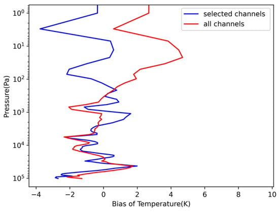
Figure 12.
Bias of Temperature in selected channels and all channels.
Currently, the microwave sensor has fewer channels but has achieved good results. Some researchers believe that the data generated by hyperspectral sensors are too large, leading to a burden on retrieval calculations. However, Yanmeng Bi [14] and his colleagues have verified that microwave satellites have many potential advantages for hyperspectral applications. For example, they can mitigate radio frequency interference (RFI), improve the certainty of inference for line strength and width, and facilitate inversion and modeling. In Figure 13, it can be observed that we compared a CNN network with five convolutional layers to CNN-LAA. Within the same training time, CNN-LAA demonstrated a faster training speed, reaching a smaller loss value when stabilized. This method is suitable for addressing the issue of high computational resource consumption due to the large data volume generated by hyperspectral sensors.
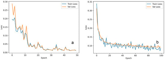
Figure 13.
(a) CNN-LAA training loss (blue line) and validation loss (yellow line) with epochs, and (b) shows CNN losses.
Furthermore, this method is beneficial in practical engineering applications for reducing the influence of noise on the model, improving model robustness, and enhancing generalization capability. After the convolution and attention operations, the model also incorporates two fully connected layers and dropout layers to enhance the nonlinear fitting ability and stability. Our paper utilizes the Adaptive Moment Estimation (Adam) optimization algorithm [32], which combines the ideas of momentum gradient descent and RMSprop. Adam can adaptively adjust the learning rates for each hyperparameter and introduces a momentum term for smooth parameter updates.
6. Conclusions
This study proposes a CNN-LAA algorithm for hyperspectral microwave temperature retrieval, which not only improves accuracy but also performs better in handling details. The article first optimizes the hyperspectral microwave channels based on information content, selecting 268 channels containing 90% of the information distributed around 60 GHz, 118 GHz, and 425 GHz. Then, the dataset is input into ARTS to simulate the corresponding brightness temperatures. Through the validation of the test set, the method achieves excellent retrieval results, with an RMSE of 1.46 K and an MAE of 1.40 K for temperature retrieval, outperforming the 1D-CNN, Attention, BPNN, XGBoost, and SVM methods at their best levels. In terms of handling details, CNN-LAA outperforms other methods, particularly demonstrating better robustness in the middle and upper atmospheric layers. This study demonstrates the effectiveness of the CNN-LAA approach for hyperspectral microwave temperature retrieval, which can capture subtle changes in atmospheric conditions, aiding in the understanding of atmospheric structures and enhancing the accuracy of weather forecasting. While improving the retrieval accuracy, this method can be extended to three-dimensional space and still perform well in complex scenarios, with errors controlled within 0.7 K, providing a new reference method for research on and the design of satellite-based hyperspectral microwave radiometers. In more intricate environments and simulated instrument scenarios, the model exhibits a more notable enhancement in accuracy, providing valuable assistance for future satellite multi-channel selection. This paper only discusses the application of this method in retrieving temperature profiles under clear-sky conditions, without considering cloud scattering effects, which can have a significant impact on the profiles. And we did not evaluate the impact of data uncertainty on the performance of the retrieval method. The uncertainty in the dataset might affect the selection of frequency channels. Numerical simulations could be conducted by adding random noise to each channel to obtain an appropriate channel set. These could be topics for future research.
Author Contributions
Methodology, software visualization and writing original draft, X.T.; Supervision, K.M.; Analysis and investigation, F.D. All authors have read and agreed to the published version of the manuscript.
Funding
This work was supported in part by the National Natural Science Foundation of China for Key Project under Grant 61831017, in part by the National Key Research and Development Program of China under Grant 2018YFB2202500.
Institutional Review Board Statement
Not applicable.
Informed Consent Statement
Not applicable.
Data Availability Statement
The data presented in this study are available on request from the corresponding author. The data are not publicly available due to access restrictions for some data.
Conflicts of Interest
The authors declare no conflicts of interest.
References
- Westwater, E.R. Ground-Based Passive Probing Using the Microwave Spectrum of Oxygen. J. Res. Natl. Bur. Stand. Sect. D Radio Sci. 1965, 69, 1201. [Google Scholar] [CrossRef]
- Westwater, E.R.; Sweezy, W.B.; McMillin, L.M.; Dean, C. Determination of Atmospheric Temperature Profiles from a Statistical Combination of Ground-Based Profiler and Operational NOAA 6/7 Satellite Retrievals. J. Clim. Appl. Meteorol. 1984, 23, 689–703. [Google Scholar] [CrossRef][Green Version]
- Troitsky, A.; Gajkovich, K.P.; Gromov, V.; Kadygrov, E.; Kosov, A. Thermal Sounding of the Atmospheric Boundary Layer in the Oxygen Absorption Band Center at 60 GHz. IEEE Trans. Geosci. Remote Sens. 1993, 31, 116–120. [Google Scholar] [CrossRef]
- Massaro, G.; Stiperski, I.; Pospichal, B.; Rotach, M.W. Accuracy of Retrieving Temperature and Humidity Profiles by Ground-Based Microwave Radiometry in Truly Complex Terrain. Atmos. Meas. Tech. 2015, 8, 3355–3367. [Google Scholar] [CrossRef]
- Xia, J.; Liu, Q.; Tan, L. A Deep Learning Method Integrating Multisource Data for ECMWF Forecasting Products Correction. IEEE Geosci. Remote Sens. Lett. 2023, 20, 1002105. [Google Scholar] [CrossRef]
- Gaikovich, K.P.; Markina, N.N.; Naumov, A.P.; Plechkov, V.M.; Sumin, M.I. Investigation of Remote Sensing Possibilities of the Lower Atmosphere in the Microwave Range and Some Aspects of Statistical Data Use. Int. J. Remote Sens. 1983, 4, 419–431. [Google Scholar] [CrossRef]
- Askne, J.; Skoog, G.; Winberg, E. Test of a Ground-Based Microwave Radiometer for Atmospheric Temperature Profiling with Meteorological Applications. Int. J. Remote Sens. 1985, 6, 1241–1256. [Google Scholar] [CrossRef]
- Blackwell, W.J. An Overview of the NASA Tropics Earth Venture Mission. In Proceedings of the 2017 IEEE International Geoscience and Remote Sensing Symposium (IGARSS), Fort Worth, TX, USA, 23–28 July 2017; pp. 5934–5937. [Google Scholar]
- Lipton, A.E. Satellite Sounding Channel Optimization in the Microwave Spectrum. IEEE Trans. Geosci. Remote Sens. 2003, 41, 761–781. [Google Scholar] [CrossRef]
- Blackwell, W.J.; Bickmeier, L.J.; Leslie, R.V.; Pieper, M.L.; Samra, J.E.; Surussavadee, C.; Upham, C.A. Hyperspectral Microwave Atmospheric Sounding. IEEE Trans. Geosci. Remote Sens. 2011, 49, 128–142. [Google Scholar] [CrossRef]
- Liu, D.; Lv, C.; Liu, K.; Xie, Y.; Miao, J. Retrieval Analysis of Atmospheric Water Vapor for K-Band Ground-Based Hyperspectral Microwave Radiometer. IEEE Geosci. Remote Sens. Lett. 2014, 11, 1835–1839. [Google Scholar] [CrossRef]
- Mahfouf, J.-F.; Birman, C.; Aires, F.; Prigent, C.; Orlandi, E.; Milz, M. Information Content on Temperature and Water Vapour from a Hyper-Spectral Microwave Sensor. Q. J. R. Meteorol. Soc. 2015, 141, 3268–3284. [Google Scholar] [CrossRef]
- Aires, F.; Prigent, C.; Orlandi, E.; Milz, M.; Eriksson, P.; Crewell, S.; Lin, C.-C.; Kangas, V. Microwave Hyperspectral Measurements for Temperature and Humidity Atmospheric Profiling from Satellite: The Clear-Sky Case. J. Geophys. Res. Atmos. 2015, 120, 11334–11351. [Google Scholar] [CrossRef]
- Bi, Y.; Yang, J.; Wei, C.; Dou, F.; Xu, W.; An, D.; Luan, Y.; Feng, J.; Zhang, L. Atmospheric Temperature Measurements Using Microwave Hyper-Spectrum from Geostationary Satellite: Band Design, Weighting Functions and Information Content. Remote Sens. 2024, 16, 289. [Google Scholar] [CrossRef]
- Huang, H.-L.; Antonelli, P. Application of Principal Component Analysis to High-Resolution Infrared Measurement Compression and Retrieval. J. Appl. Meteorol. Climatol. 2001, 40, 365–388. [Google Scholar] [CrossRef]
- Sica, R.J.; Haefele, A. Retrieval of Temperature from a Multiple-Channel Rayleigh-Scatter Lidar Using an Optimal Estimation Method. Appl. Opt. 2015, 54, 1872–1889. [Google Scholar] [CrossRef] [PubMed]
- Hewison, T.J. 1D-VAR Retrieval of Temperature and Humidity Profiles from a Ground-Based Microwave Radiometer. IEEE Trans. Geosci. Remote Sens. 2007, 45, 2163–2168. [Google Scholar] [CrossRef]
- Churnside, J.H.; Stermitz, T.A.; Schroeder, J.A. Temperature Profiling with Neural Network Inversion of Microwave Radiometer Data. J. Atmos. Ocean. Technol. 1994, 11, 105–109. [Google Scholar] [CrossRef]
- Jiang, N.; Xu, Y.; Xu, T.; Li, S.; Gao, Z. Land Water Vapor Retrieval for AMSR2 Using a Deep Learning Method. IEEE Trans. Geosci. Remote Sens. 2022, 60, 5803011. [Google Scholar] [CrossRef]
- Rysman, J.-F.; Claud, C.; Dafis, S. A Machine Learning Algorithm for Retrieving Cloud Top Height with Passive Microwave Radiometry. IEEE Geosci. Remote Sens. Lett. 2022, 19, 4500605. [Google Scholar] [CrossRef]
- Yan, X.; Liang, C.; Jiang, Y.; Luo, N.; Zang, Z.; Li, Z. A Deep Learning Approach to Improve the Retrieval of Temperature and Humidity Profiles from a Ground-Based Microwave Radiometer. IEEE Trans. Geosci. Remote Sens. 2020, 58, 8427–8437. [Google Scholar] [CrossRef]
- Yu, W.; Xu, X.; Jin, S.; Ma, Y.; Liu, B.; Gong, W. BP Neural Network Retrieval for Remote Sensing Atmospheric Profile of Ground-Based Microwave Radiometer. IEEE Geosci. Remote Sens. Lett. 2022, 19, 4502105. [Google Scholar] [CrossRef]
- MacKinnon, J.; Gambacorta, A.; Piepmeier, J.; Stephen, M.; Kroodsma, R.; Santanello, J.; Blumberg, G.; Blaisdell, J.; Moradi, I.; Gong, J.; et al. Deep Neural Networks For Evaluating Future Satellite-Based Hyperspectral Microwave Sensor Designs. In Proceedings of the IGARSS 2023—2023 IEEE International Geoscience and Remote Sensing Symposium, Pasadena, CA, USA, 16–21 July 2023; IEEE: Piscataway, NJ, USA, 2023; pp. 5210–5213. [Google Scholar]
- Eriksson, P.; Buehler, S.A.; Davis, C.P.; Emde, C.; Lemke, O. ARTS, the Atmospheric Radiative Transfer Simulator, Version 2. J. Quant. Spectrosc. Radiat. Transf. 2011, 112, 1551–1558. [Google Scholar] [CrossRef]
- Rodgers, C.D. Information Content and Optimisation of High Spectral Resolution Remote Measurements. Adv. Space Res. 1998, 21, 361–367. [Google Scholar] [CrossRef]
- Orescanin, M.; Petkovic, V.; Powell, S.W.; Marsh, B.R.; Heslin, S.C. Bayesian Deep Learning for Passive Microwave Precipitation Type Detection. IEEE Geosci. Remote Sens. Lett. 2022, 19, 4500705. [Google Scholar] [CrossRef]
- Ioffe, S.; Szegedy, C. Batch Normalization: Accelerating Deep Network Training by Reducing Internal Covariate Shift. In Proceedings of the 32nd International Conference on Machine Learning, PMLR, Lille, France, 6–11 July 2015. [Google Scholar]
- Han, D.; Ye, T.; Han, Y.; Xia, Z.; Song, S.; Huang, G. Agent Attention: On the Integration of Softmax and Linear Attention. arXiv 2023, arXiv:2312.08874. [Google Scholar]
- Varghese, A.A.; Krishnadas, J.; Antony, A.M. Robust Air Quality Prediction Based on Regression and XGBoost. In Proceedings of the 2023 Advanced Computing and Communication Technologies for High Performance Applications (ACCTHPA), Ernakulam, India, 20–21 January 2023; pp. 1–6. [Google Scholar]
- Gong, A.; Liu, W.; Shan, Y.; Chen, X.; Yue, J. Retrieval of Land Surface Temperature (LST) Based on Support Vector Machine (SVM) from HJ-1B Data with Single-Channel. In Proceedings of the 2012 IEEE International Geoscience and Remote Sensing Symposium, Munich, Germany, 22–27 July 2012; pp. 4229–4232. [Google Scholar]
- Wang, D.; Tong, L.; Gong, X.; Guan, X.; Wang, P.; Gao, B. Retrieval of Atmospheric Temperature Profiles from Hyperspectral Microwave Radiative Data Based on the Neural Network. In Proceedings of the 2021 IEEE International Geoscience and Remote Sensing Symposium IGARSS, Brussels, Belgium, 11–16 July 2021; pp. 7095–7098. [Google Scholar]
- Kingma, D.P.; Ba, J. Adam: A Method for Stochastic Optimization. arXiv 2017, arXiv:1412.6980. [Google Scholar]
Disclaimer/Publisher’s Note: The statements, opinions and data contained in all publications are solely those of the individual author(s) and contributor(s) and not of MDPI and/or the editor(s). MDPI and/or the editor(s) disclaim responsibility for any injury to people or property resulting from any ideas, methods, instructions or products referred to in the content. |
© 2024 by the authors. Licensee MDPI, Basel, Switzerland. This article is an open access article distributed under the terms and conditions of the Creative Commons Attribution (CC BY) license (https://creativecommons.org/licenses/by/4.0/).