An Ensemble-Based Model for Specific Humidity Retrieval from Landsat-8 Satellite Data for South Korea

Abstract

Specific humidity (SH) which means the amount of water vapor in 1 kg of air, is used as an indicator of energy exchange between the atmosphere and the Earth’s surface. SH is typically computed using microwave satellites. However, the spatial resolution of data for microwave satellite is too low. To overcome this disadvantage, we introduced new methods that applied data collected by the Landsat-8 satellite with high spatial resolution (30 m), a meteorological model, and observation data for South Korea in 2016–2017 to 4 machine learning techniques to develop an optimized technique for computing SH. Among the 4 machine learning techniques, the random forest-based method had the highest accuracy, with a coefficient of determination (R) of 0.98, Root Mean Square Error (RMSE) of 0.001, bias of 0, and Relative Root Mean Square Error (RRMSE) of 11.16%. We applied this model to compute land surface SH using data from 2018 to 2019 and found that it had high accuracy (R = 0.927, RMSE = 0.002, bias = 0, RRMSE = 28.35%). Although the data used in this study were limited, the model was able to accurately represent a small region based on an ensemble of satellite and model data, demonstrating its potential to address important issues related to SH measurements from satellites.

1. Introduction

The relationship between the atmosphere and the Earth’s surface influences weather conditions; sensible and latent heat transfer from the surface to the air account for a significant portion of the energy input to the atmosphere [1]. And moisture in the atmosphere is among the most important factors in this relationship. As a greenhouse gas, water vapor strongly influences the surface radiation budget and therefore the temperature and water cycle [2]. Moisture in the atmosphere near the surface supplies additional water vapor to the upper atmosphere through vertical mixing, creating a positive feedback effect. Accurate measurement of this moisture is essential for predicting and preparing for extreme weather events such as droughts, which directly affect agricultural crop production [3,4,5]. For example, previous study noted that 70% of the temperature increase in Europe was associated with a rapid increase in atmospheric moisture in Central Europe [2,6]. However, atmospheric moisture is characterized by high daily, annual, and spatial variability [2,7,8,9]. Therefore an accurate spatial representation of atmospheric moisture is very important. This representation of atmospheric moisture can be expressed in several ways, including relative humidity and Specific Humidity (SH). SH is the mass (g) of water vapor contained in 1 kg of total (wet) air, and it strongly influences the radiation budget at the Earth’s surface [3,4,5]. The accuracy of SH measurements affects that of data retrievals used in meteorological models such as convolutional long short-term memory and Numerical Weather Prediction (NWP) models [10,11,12]. In the field of satellite remote sensing, SH has been used as validation data for satellite measurements, including output from the Communication Oceanographic and Meteorological Satellite/Meteorological Imager (COMS/MI). Currently, studies of SH computation in remote sensing have been conducted for the atmosphere over the ocean, but studies of SH over land tend to be relatively scarce because it is difficult to obtain accurate values of SH near the surface [5,13,14]. Studies of SH over land have typically been conducted using radiometers, which are geographically limited because SH measurements can only be made in the area of the radiometer’s actual installation. Therefore, early attempts to compute land surface SH data were based on empirical relationships between average monthly precipitation and in-situ SH observations [15,16,17]. Later, a method was developed to obtain SH data by estimating the amount of water vapor using specialized sensor microwaves/imagers (SSM/I) [18]. Based on this, most of the later satellite-based SH calculation studies were performed using microwave sensors. Although studies using microwave sensors are meaningful as measurements over a wide range, the spatial resolution is over 20 km, so there are limitations in using such data for areas such as urban areas that contain many spatial structures in a small area. To overcome this limitation, it is essential to use materials with high spatial resolution. And we thought if SH can be computed with high spatial resolution, it can be used as an input to the various model such as Computational Fluid Dynamics model. And This is very useful when studying small areas that require high-resolution data. Therefore, we developed a method to compute SH by applying data ensemble of Landsat-8 satellite data and meteorological model data to an ML algorithm in this study. This method can achieves a high spatial resolution of 30 m, which is better than previous studies using microwaves. This high spatial resolution is particularly advantageous for analyzing areas with small and complex structures such as urban area.

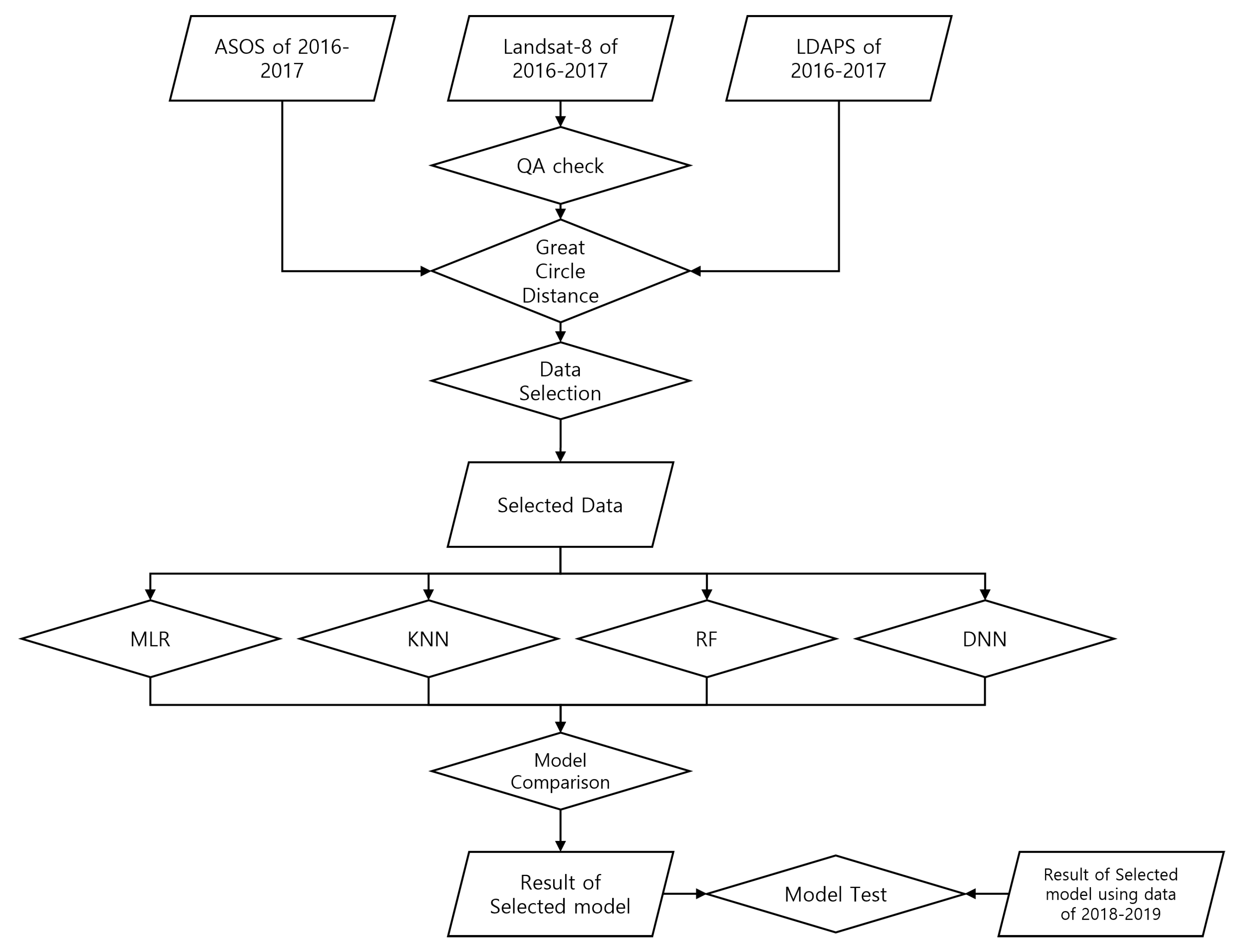
2. Materials and Methods

2.1. Study Area

The study area included South Korea, extending from about 33° N to 39° N and from 124° E to 130° E. South Korea is part of Northeast Asia, which experiences four seasons with considerably different characteristics regarding atmospheric readings. There are four air masses that affect the seasons of South Korea: the North Pacific air mass, characterized by a very high temperature and very high humidity in summer; the Siberian air mass, characterized by a very low temperature and low humidity in winter; the Yangtze-river air mass, which comes from China and brings warm temperatures in spring and autumn; and the Okhotsk Sea air mass, characterized by cool temperatures and high humidity. The Okhotsk Sea air mass brings rain to South Korea during the rainy season in summer and early autumn. Additionally, South Korea is surrounded on three sides by the sea; thus, both land and sea conditions affect the region’s humidity. And especially, previous studies referred effect to cold surges by arctic oscillation [19,20]. We thought if we can retrieve SH from satellite, the result can be used to analyze change of humidity in large area. For this reason, we chose South Korea as our study area to retrieve SH on the period from 2016 to 2019 for the corresponding spatial range.

2.2. Materials

2.2.1. Data from Direct Measurement

In this study, we utilized data from the Automated Synoptic Observing System (ASOS), which consists of in-situ data collected by the Korea Meteorological Administration (KMA). ASOS comprises 102 measurement sites across South Korea, generating a comprehensive set of meteorological observations on an hourly basis (Figure 1). In this study, we used on the 2:00 (UTC) data, which aligns with the optimal observation time for Landsat-8 satellite imagery. It’s worth noting that ASOS does not directly provide specific data for specific humidity (SH). To overcome this limitation, we computed the specific humidity using atmospheric pressure and water vapor pressure data collected by ASOS. This computation method, as suggested by Bolton [21], is as follows:

$$SH=622e/(p-378e)$$

(1)

where p is air pressure (hpa) and e is vapor pressure (hpa).

This approach allowed us to derive the specific humidity values required for our analysis, ensuring the compatibility of the ASOS data with our research objectives.

2.2.2. Data from Satellite

The Landsat-8 satellite, operated by the United States Geological Survey (USGS), observes the Earth on 4 visible and 3 infrared wavelength bands at a spatial resolution of 30 m and two thermal infrared (TIR) wavelength bands at a spatial resolution of 100 m and USGS provides TIR data re-sampled to 30 m. USGS provides top-of-canopy surface reflectance data corrected using Landsat-8 atmospheric observations; the data show surface reflectance with atmospheric effects such as clouds, water vapor, and ozone removed. In this study, we used 7 band data of Landsat-8 data for satellite data (Band 2(Blue), Band 3(Green), Band 4(Red), Band 5(NIR), Band 6(SWIR1), Band 10(TIR1), Band 11(TIR2)).

The normalized difference vegetation index (NDVI) uses differences between Red (0.64–0.67 $\mathsf{\mu }$m) and Near-InfraRed (NIR; 0.85–0.88 $\mathsf{\mu }$m) reflectance observations to distinguish vegetation coverage, as follows:

$$NDVI=(NIR-Red)/(NIR+Red)$$

(2)

For dense vegetation cover, NIR reflectance is high, leading to high NDVI values; conversely, sparse vegetation cover produces low NDVI values. Thus, NDVI has often been applied to resolve land surface changes related to global climate change, the carbon cycle, land coverage/use, and terrestrial ecology [22,23]. Because vegetation and moisture are closely related, we assumed that NDVI and SH would be strongly correlated; therefore, we used NDVI as a input parameter for the model used in this study. We computed NDVI for each pixel, and the pixel data were verified against quality assurance (QA) data prior to further computations.

The normalized difference water index (NDWI) represents surface water conditions; the first NDWI was based on NIR and short-wave IR, and the second used green and NIR wavelengths [24,25]. Our approach for inferring the surface moisture of a pixel was based on the Gao method, which is commonly used in remote exploration [26,27]. We computed NDWI using the Green (0.53–0.59 $\mathsf{\mu }$m) and Shortwave IR 1 (SWIR; 1.57–1.65 $\mathsf{\mu }$m) wavelengths for each pixel as follows:

$$NDWI=(SWIR1-Green)/(SWIR1+Green)$$

(3)

The resulting NDWI pixel data were cross-checked against QA data. And in this study, we utilized NDWI as a input parameter for the model.

We used surface EMIssivity (EMI) data which were obtained from 2 of InfraRed bands (11 $\mathsf{\mu }$m and 12 $\mathsf{\mu }$m) for Land Surface Temperature (LST) computations as a input parameter not to the model. We computed EMI as suggested by previous paper [28].

$$\epsilon 10=0.9897+0.029\ast ln\left(NDVI\right)$$

(4)

$$\epsilon 10-\epsilon 11=0.01019+0.01344\ast ln\left(NDVI\right)$$

(5)

We optimized the Landsat-8 based LST data using the Prata method [29], as follows:

$$LST=3.45\ast \frac{T10-273.15}{\epsilon 10}-2.45\ast \frac{T11-273.15}{\epsilon 11}+40\ast \frac{1-\epsilon 10}{\epsilon 10}+273.15$$

(6)

where $\epsilon$10 and $\epsilon$11 are the EMI, T11 and T12 are brightness temperature of 11 $\mathsf{\mu }$m and 12 $\mathsf{\mu }$m band data, respectively.

The Solar Zenith Angle (SZA) is defined as the angle between the zenith point directly above a specific location on the Earth’s surface and the line of sight extending from that location to the sun. Typically, the SZA is employed in conjunction with the Solar Azimuth Angle (SAA) to determine the precise position of the sun relative to a specific location on the Earth’s surface. Thus, both SZA and SAA undergo variations relative to the sun’s and satellite’s positions, and these fluctuations constitute a vital aspect of satellite imagery, as they have a direct impact on the reflectance characteristics of the Earth’s surface. In our study, we computed these values based on observation times and latitudes, incorporating them as input parameters for the model.

2.2.3. Data from Weather Prediction Model

The Korea Meteorological Administration (KMA) has been operating a weather forecast system based on the Unified Model developed by the Met Office since 2015. For this research, we utilized data from the Local Data Assimilation and Prediction System (LDAPS), which offers hourly data with spatial resolution of 1.5 km. Ta and DT are known to exhibit a strong correlation with atmospheric moisture. As a result, we incorporated Ta and DT as critical input variables for our analysis, recognizing their significance in characterizing atmospheric moisture conditions. When using only satellite data, sufficient accuracy may not be secured due to insufficient input data. Therefore, this study attempted to compensate for this weakness by using meteorological model data as input parameters.

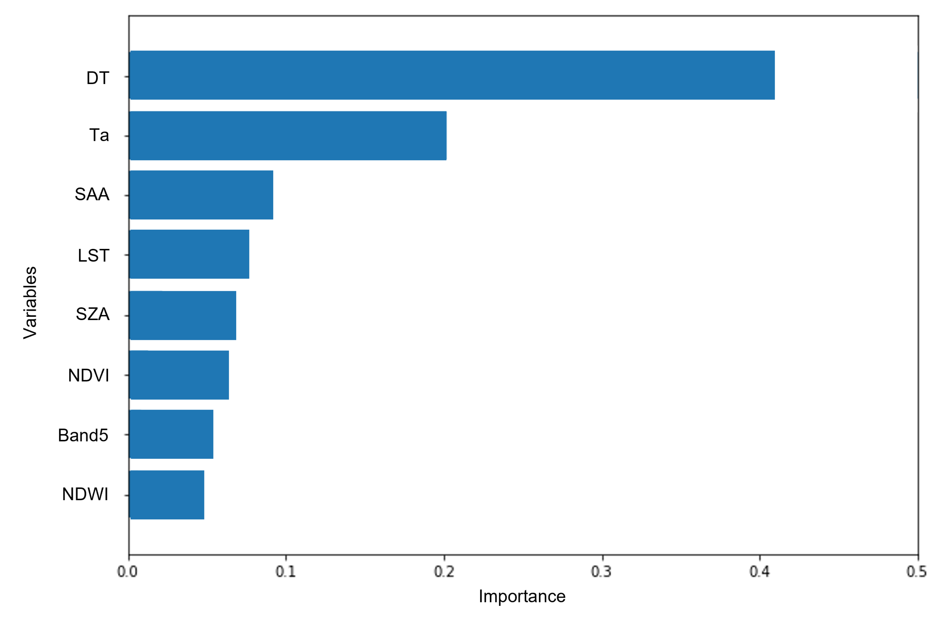
2.3. Variables Selection

The quality of the computed SH has the greatest influence on the accuracy of the optimal input variables. Incorrect data input may cause noise during the computation process, lowering accuracy and lengthening the computation time. Therefore, correlation analysis was performed between the ASOS-derived SH and each type of input data, and the values of Pearson’s correlation coefficient (R) were compared to select the appropriate input variable for the model, as described in a previous ML study [30,31]. The results showed that R ranged from −0.768 to 0.976 (

Table 1. Correlation coefficient between SH and each variable.

Variables	R	Selection	Variables	R	Selection
Band 1	−0.18	X	NDWI	0.613	O
Band 2	−0.233	X	SZA	−0.644	O
Band 3	−0.061	X	SAA	−0.768	O
Band 4	−0.39	X	LST	0.882	O
Band 5	0.621	O	Ta	0.914	O
Band 6	0.05	X	DT	0.976	O
Band 7	−0.232	X	Soil Moisture	−0.433	X
NDVI	0.689	O	Air Pressure	−0.433	X

). Generally, R value of 0.6 or higher is considered a moderate positive correlation, and an R value of 0.8 or higher is considered a strong positive correlation [32]. Therefore, we evaluated variables with |R| > 0.6 as appropriate input variables. As a result, we selected bands 5, NDVI, NDWI, SZA, SAA, LST, Ta and DT as model input parameters.

2.4. Methods

The primary objective of this study is to derive highly accurate Specific Humidity (SH) data by employing a variety of Machine Learning (ML) methods, incorporating data from satellite sources, model data, and ground-based measurements (Figure 2). This methodology involved the application of various regression techniques to computed SH. First of all, pixels were selected for good, clear sky condition data using the Landsat-8 QA product, and satellite-based input data were produced using the corresponding data. It is important to match the three types of data used in this study, Landsat-8 data, ASOS data, LDAPS data, exhibited temporal and spatial disparities due to differences in their acquisition characteristics. To match for these temporal variations, we specifically focused on data collected closest to 02:00 UTC, which aligns with the observation time of Landsat-8 over the study area. Additionally, to rectify spatial discrepancies stemming from the varying spatial resolutions of Landsat-8 and LDAPS data, we employed the Great Circle Distance (GCD) method. This method enabled us to select the nearest pixels from both Landsat-8 and LDAPS data in relation to the ASOS observation points. These adjustments were undertaken to ensure the coherence and consistency of the data sources used in our analysis.

To retrieve Specific Humidity (SH), we used a ensemble of satellite data (including bands 5, NDVI, NDWI, SZA, SAA, and LST) and weather prediction model data (Ta and DT), applying 4 machine learning algorithms: Multiple Linear Regression (MLR), K-Nearest Neighbors (KNN), Random Forest (RF), and Deep Neural Network (DNN).

For training each model, we used from 2016 to 2017, which are 4005 SH measurements obtained from ASOS as the dependent variable, while the independent variables included six satellite data parameters (bands 5, NDVI, NDWI, SZA, SAA, LST) and two weather model data variables (Ta, DT), resulting in a dataset of 24,030. To identify the optimal SH model, we followed a robust approach: we trained the models on 70% of the data and selected the best-performing model based on the remaining 30%. This training phase utilized 2083 SH measurements and 16,821 satellite and meteorological model data points.To enhance the models’ performance and address issues like multicollinearity and overfitting, we incorporated optimization techniques such as dropout, L1 or L2 regularization, and early stopping, as recommended by prior research [33,34].

The previously set 30% validation data of 7209 satellite and weather model data points were then applied to the trained model to compute 1202 SH. These computed SH were then validated by comparing them to the directly measured SH in ASOS to evaluate the optimal model for each method.

The selected optimal model allowed us to compute SH with the same dimensions as Landsat-8. We applied this model to data spanning from 2018 to 2019 and compared the computed SH values with those measured by ASOS during the same period to confirm the accuracy of our approach.

2.4.1. Multiple Linear Regression Algorithm

MLR extends simple linear regression for use with multiple variables. In both types of regression, the response variable is assumed to be directly related to a linear combination of the explanatory variables [35]. In this study, MLR was the first technique used to compute SH, using ASOS-based SH as the independent variable and 8 input variables. The remaining 30% of the satellite and meteorological model data was input into the model produced using 70% of the data to compute the SH data, and validation was performed by comparing the data with the actually measured ASOS SH data.

2.4.2. K-Nearest Neighbor Algorithm

KNN regression is a non-parametric regression analysis that predicts the amount of a predictor in real time by applying information derived from observed data without defining a predetermined parametric relationship between data [36,37]. The KNN algorithm interpolates field properties by considering the k-nearest neighbors based on an n-dimensional space.

In this study, SH was computed by applying the KNN algorithm to the optimal variables. The model was run by setting k to values from 1 to 20. For all k-value ranges accuracy showed R-value greater than 0.94 and an RMSE less than 0.016, and we chose the optimal k value 6 yields the most accurate result.

2.4.3. Random Forest Algorithm

RF regression is a supervised learning algorithm that uses ensemble learning methods, which combine predictions from variable ML algorithms to create more accurate predictions than a single model [38,39]. To determine hyper-parameter conditions to produce the most accurate results, RF models having 10–1000 decision trees were validated. All of them showed high accuracy which have R-value greater than 0.95 and an RMSE less than 0.015. As a result, RF model which had 120 trees which showed the highest accuracy, was selected in this study. And Individual decision trees typically can exhibit high variance and tend to overfit. To resolve overfitting, we used the injected randomness in forests yield decision trees with somewhat decoupled prediction errors. By taking an average of those predictions, we thought that errors can cancel out.

2.4.4. Deep Neural Network Algorithm

DNN algorithms are based on artificial neural networks, which are created by imitating the structure of a human neural network. Like the human brain, weights are applied to input data to produce the output [40]. For training step, we used a rectified linear unit (ReLU) activation function, and the number of hidden layers was set in the range of 4 to 6. The ReLU activation function was applied one to three times for each hidden layer. It is worth noting that the ReLU activation function can effectively approximate a linear finite element function, especially when multiple layers (at least two) are used, as suggested by previous research [41]. For our optimisation, we utilised the ADAM optimiser, which is known for its adaptive learning speed, ease of implementation and computational efficiency [42]. To determine the optimal hyperparameter settings, we performed an exhaustive search using the same input data used for the other ML techniques. We used the ADAM optimiser, exploring a range of epochs from 100 to 3000 and batch sizes from 32 to 2048. We ultimately selected a configuration of epoch 100 and batch size 512 as the optimal settings for the DNN model.

3. Results

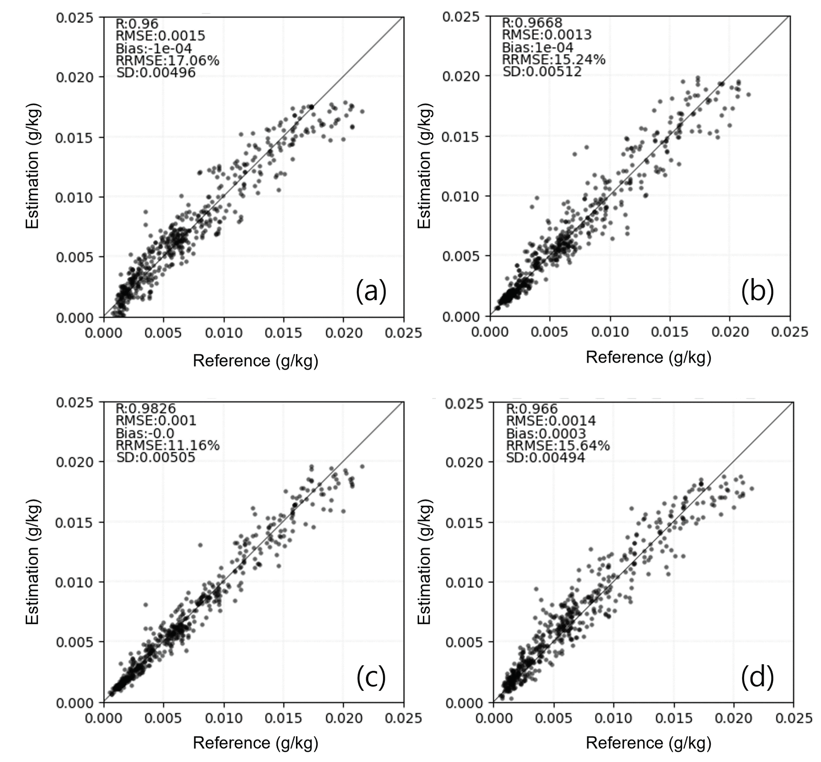
3.1. Model Comparison

For the MLR, KNN, RF, and DNN algorithms, SH was computed by applying the final input variable set determined by comparing accuracy indices for the model results. Training was performed using a random selection of 70% of the data, and the optimal model was selected by comparing the results with the remaining 30%. Previous studies have evaluated SH model results using only R and the root mean square error (RMSE); however, SH values at the surface are much lower than those obtained in studies conducted at sea level [13,14]. Therefore, we evaluated model accuracy according to the relative RMSE (RRMSE) as well as R, RMSE, bias, and Standard Deviation (SD) (Figure 2,

Table 2. Comparison with Results of validation of 4 machine learning methods.

	Mutiple Linear Regression	K-Nearest Neighbor	Random Forest	Deep Neural Network
R	0.96	0.9668	0.9826	0.966
RMSE (g/kg)	0.0015	0.0013	0.001	0.0014
Bias (g/kg)	−0.0001	0.0001	0	0.0003
RRMSE (%)	17.06	15.24	11.16	15.64
SD (g/kg)	0.00496	0.00512	0.00505	0.00494

). The accuracy indices of the MLR algorithm were as follows: R = 0.96, RMSE = 0.0015, bias = 0, RRMSE = 17.06%, and SD = 0.00496. The KNN algorithm resulted in R = 0.9668, RMSE = 0.0013, bias = 0, RRMSE = 15.24% and SD = 0.00512. The RF algorithm resulted in R = 0.9826, RMSE = 0.001, bias = 0, RRMSE = 11.16%, and SD = 0.00505. The DNN resulted in R = 0.966, RMSE = 0.0014, bias = 0.0003, RRMSE = 15.64%, and SD = 0.00494. A comparison of the R, RMSE, and RRMSE values indicated that model accuracy descended in the order RF, KNN, DNN, MLR except SD. In these results, R, RMSE, Bias, SD were showed similar values and RRMSE values showed a relatively large difference. Therefore, RF was determined to be the most appropriate SH computation model (Figure 3 and Figure 4). And the importance of input variables was evaluated using the GINI coefficient through the method in the references [43,44], and the importance was in the order of DT, Ta, SAA, LST, SZA, NDVI, Band 5, and NDWI, with the highest correlation DT had the highest importance (Figure 5). DT is an input variable that must be included in SH computation, and we thought that other variables had sufficient influence.

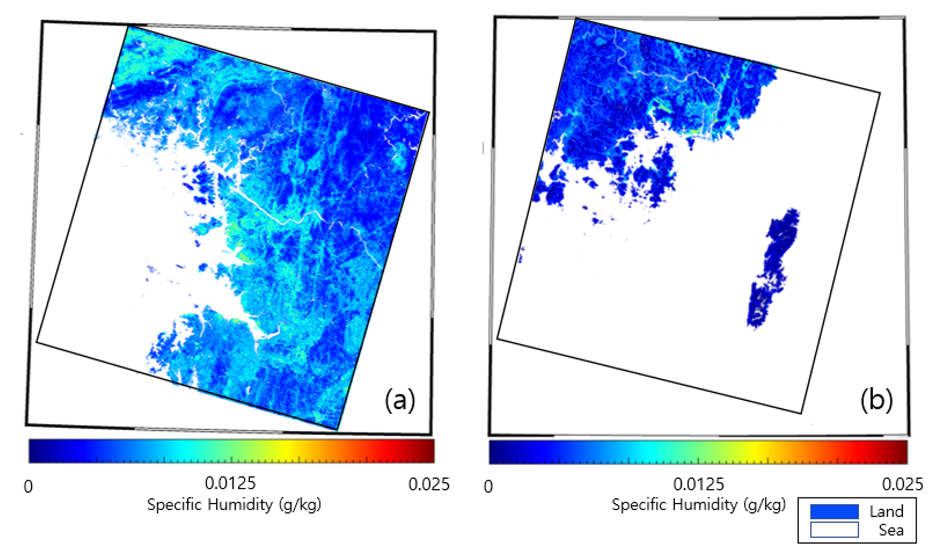
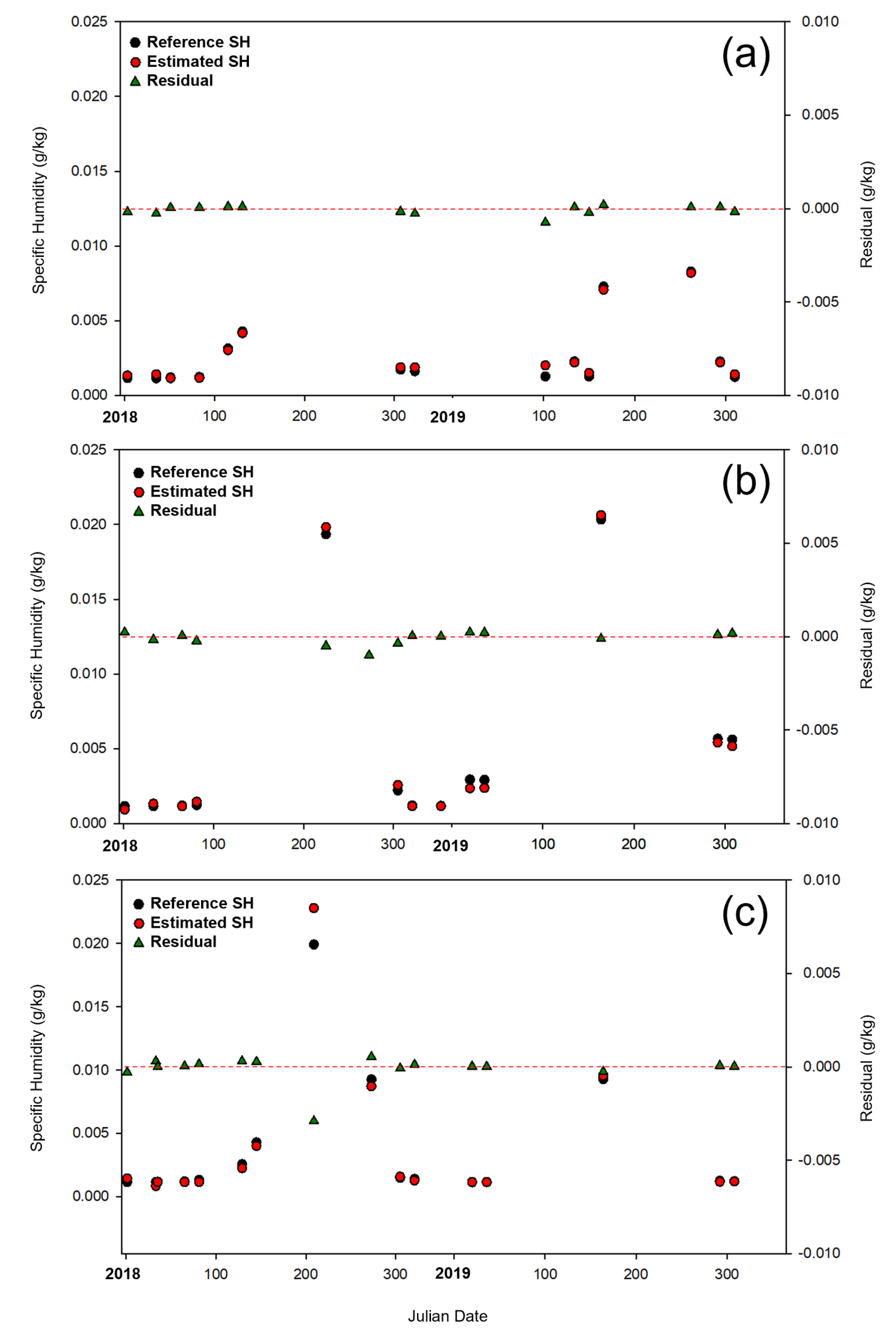
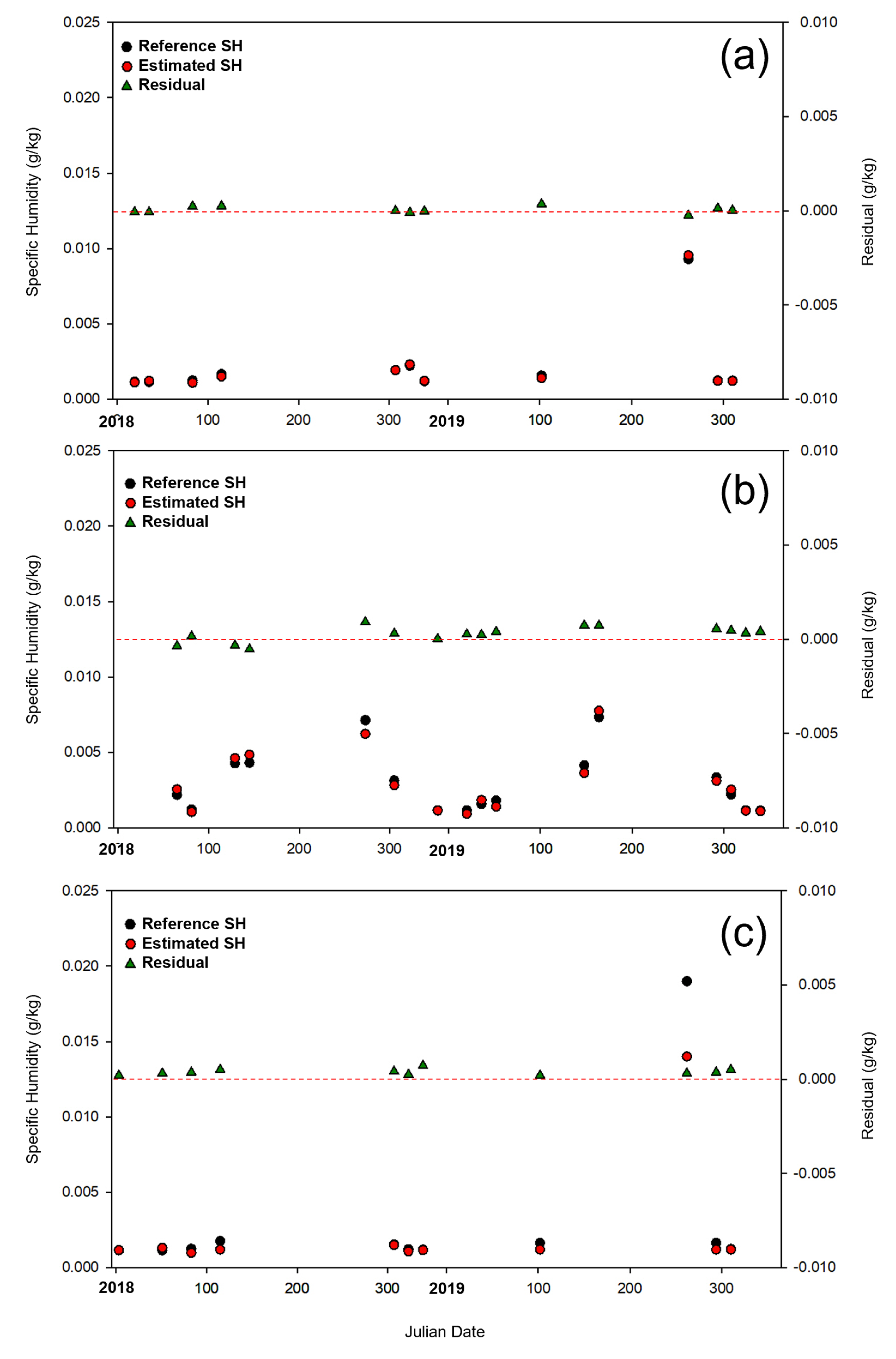
3.2. Model Test Using ASOS Point from 2018 to 2019

Typically, data are divided into training, validation, and testing sets in ML studies. But, we performing training and validation using data from 2016 to 2017, and testing using ASOS observations and six satellite data parameters (bands 5, NDVI, NDWI, SZA, SAA, LST) and two weather model data variables (Ta, DT) from 2018 to 2019 in this study. First, we checked the accuracy of the RF model using data from 2018 to 2019. The data applied to the selected RF model and the results were compared to ASOS SH (Figure 6). The R was 0.9273, RMSE was 0.002, Bias was 0.0001, RRMSE was 28.35% and SD was 0.004. Their accuracy was a little lower than the training step, but we thought they showed good accuracy. This means the model can be used to compute SH for various periods. And the second testing was conducted using a total of six datasets corresponding to Seoul (Figure 7a), Busan (Figure 7b), Incheon (Figure 7c), Andong (Figure 8a), Gyeongju (Figure 8b), and Chuncheon (Figure 8c). Seoul data were used to test SH computation accuracy for urban areas, and Busan and Incheon data were used to test SH computation accuracy for high-moisture conditions, due to their proximity to the sea. Gyeongju data were used to test SH computation accuracy for regions with rich vegetation because the area around the observation station was forested. Andong and Chuncheon data were used to test SH computation accuracy for agricultural areas. The testing results indicated that all six regions had higher SH values (0.08–0.19) from June to September due to the effects of a warm, humid North Pacific air mass than in other periods, due to a cool, dry Siberian air mass from December to February. The R values for each region were 0.931 (Seoul), 0.912 (Busan), 0.8 (Incheon), 0.832 (Andong), 0.988 (Chuncheon), and 0.907 (Gyeongju), with an overall R of 0.868. The RMSE values for each region were 0.0002 (Seoul), 0.0003 (Busan), 0.0008 (Incheon), 0.0001 (Andong), 0.0001 (Chuncheon), and 0.0003 (Gyeongju), with an overall RMSE of 0.0004. Comparing these results with the model verification results, the R value was reduced by approximately 0.12 and RMSE was increased by approximately 0.0003. Although the accuracy for these tests was lower than that for the model validation results, the difference between reference and computation SH values was very low, within 0.001 in all regions (urban, high-moisture, forest, and agricultural areas) and periods. As a result, the SH model developed in this study was concluded to have high accuracy.

4. Discussion

In this study, we compared four machine learning techniques and then we selected RF model to compute surface SH based on optical satellite data. The model is computation land SH, unlike most studies that focus on the SH in the ocean. Because very few studies of land surface SH computation using satellite exist, we inevitably compare the accuracy of this study to those of ocean SH, and the results are shown in

Table 3. Comparison with previous studies.

	Jin et al. (2015) [13]	Gao et al. (2019) [14]	Jackson et al. (2009) [15]	This Study
RMSE (g/kg)	0.78	1.53	1.56∼2.11	0.001
Bias (g/kg)	-	0.17	−0.02∼0.46	0

[13,14,15]. This study showed the results in the only South Korea area, and the results showed higher accuracy in both RMSE and Bias compared to previous studies. These results showed that the machine learning model of this study used for computing specific humidity shows very good performance. The SH data in this study are expected to contribute to urban microclimate analysis by being utilized as input data for various models such as Computational Fluid Dynamics (CFD), which can produce a variety of meteorological data with high spatial resolution and high accuracy [45]. It can also help to respond to weather changes in cities such as the heat island effect.

5. Conclusions

The main objective of this study was to develop a machine learning model to calculate land surface SH with high spatial resolution using optical satellite data, which overcomes the weakness of spatial resolution of microwave sensors and aims to compute SH for areas containing various structures in a small area such as urban area. We applied machine learning to data from the Landsat-8 satellite, which has a high spatial resolution of 30 m and LDAPS, a weather model, collected in 2016 and 2017, to calculate accurate SH. 8 input variables that are highly correlated with SH were applied to MLR, KNN, RF, and DNN, and the RF model showed the best performance, which showed the highest accuracy of R (0.982), RMSE (0.001), bias (0), and RRMSE (11.45%). To test the availability of a high-performance SH calculation model, we applied the 2018–2019 data to the RF model to evaluate its accuracy. The results showed stable results of R (0.927), RMSE (0.002), bias (0), and RRMSE (28.35%). Then, to test the model performance under various atmospheric and land surface conditions, we applied the data to six ASOS point data. As a result, it showed high accuracy of R was greater than 0.868, RMSE was less than 0.0004, and the difference between the actual ASOS SH and the calculated SH was almost 0. This confirms that the RF model developed in this study perform well under various atmospheric and land surface conditions. However, there are some limitations of the proposed RF model. First, we only used data for the period of 2016–2017, so the impact of special events cannot be reflected. For example, in 2020, extreme weather events such as rainy seasons, floods, and heat waves occurred around the world, and these impacts also affected South Korea. Therefore, the model did not reflect the impacts for that period, and we recommend that models should be considered about using long-term data, including periods before 2016 and after 2017 in the future. Second, despite the high spatial resolution, it is important to recognize that this study relies on Landsat-8 data, which is limited by the relatively low temporal resolution. Because of these limitations, the results of this study are valuable as a case study, but not enough to generalize. Third, this study utilizes the four most basic types of machine learning, which has the weakness of not being able to take advantage of recent machine learning models, which means that the potential exists to produce better results. However, the main purpose of this study is to confirm that there is a potential for machine learning to be used in computing SH of the land surface. Therefore, because these limitations, we focused our research on presenting our methodology to other researchers along with ideas for calculating surface SH using optical satellite data and machine learning. Although this study is limited to Korea and has a weakness in terms of the study area, we have shown that the RF model developed in this study has sufficient performance to calculate the surface SH using satellite data, and we have also shown the possibility of calculating SH using satellite data. Based on this study, we believe that further research can be conducted to calculate various meteorological variables by applying satellite data to ML. We also expect that the various meteorological variables produced based on this study can be used as inputs to other studies or as inputs to various meteorological models and play a role in various atmospheric analyses. And we suggest that future studies should use a longer period of data and various satellite data, including Landsat-8, and use various machine learning techniques.

References

1. Jackson, D.L.; Wick, G.A.; Bates, J.J. Near-surface retrieval of air temperature and specific humidity using multisensor microwave satellite observations. J. Geophys. Res. Atmos. 2006, 111, D10306. [Google Scholar] [CrossRef]
2. Ruckstuhl, C.; Philipona, R.; Morland, J.; Ohmura, A. Observed relationship between surface specific humidity, integrated water vapor, and longwave downward radiation at different altitudes. J. Geophys. Res. Atmos. 2007, 112, D03302. [Google Scholar] [CrossRef]
3. Wizemann, H.D.; Ingwersen, J.; Högy, P.; Warrach-Sagi, K.; Streck, T.; Wulfmeyer, V. Three year observations of water vapor and energy fluxes over agricultural crops in two regional climates of Southwest Germany. Meteorol. Z. 2015, 24, 39–59. [Google Scholar] [CrossRef]
4. Augustine, J.A.; Dutton, E.G. Variability of the surface radiation budget over the United States from 1996 through 2011 from high-quality measurements. J. Geophys. Res. Atmos. 2013, 118, 43–53. [Google Scholar] [CrossRef]
5. Hartmann, D.; Ramanathan, V.; Berroir, A.; Hunt, G. Earth radiation budget data and climate research. Rev. Geophys. 1986, 24, 439–468. [Google Scholar] [CrossRef]
6. Philipona, R.; Dürr, B.; Ohmura, A.; Ruckstuhl, C. Anthropogenic greenhouse forcing and strong water vapor feedback increase temperature in Europe. Geophys. Res. Lett. 2005, 32, L19809. [Google Scholar] [CrossRef]
7. Held, I.M.; Soden, B.J. Water vapor feedback and global warming. Annu. Rev. Energy Environ. 2000, 25, 441–475. [Google Scholar] [CrossRef]
8. Dai, A.; Wang, J.; Ware, R.H.; Van Hove, T. Diurnal variation in water vapor over North America and its implications for sampling errors in radiosonde humidity. J. Geophys. Res. Atmos. 2002, 107, ACL-11-1–ACL-11-14. [Google Scholar] [CrossRef]
9. Trenberth, K.E.; Dai, A.; Rasmussen, R.M.; Parsons, D.B. The changing character of precipitation. Bull. Am. Meteorol. Soc. 2003, 84, 1205–1218. [Google Scholar] [CrossRef]
10. Tekin, S.F.; Karaahmetoglu, O.; Ilhan, F.; Balaban, I.; Kozat, S.S. Spatio-temporal weather forecasting and attention mechanism on convolutional lstms. arXiv 2021, arXiv:2102.00696. [Google Scholar]
11. Treadon, R.E.; Pan, H.L.; Wu, W.S.; Lin, Y.; Olson, W.S.; Kuligowski, R.J. Global and regional moisture analyses at NCEP. In Proceedings of the ECMWF/GEWEX Workshop on Humidity Analysis, Reading, UK, 8–11 July 2002; pp. 33–47. [Google Scholar]
12. Carminati, F.; Migliorini, S.; Ingleby, B.; Bell, W.; Lawrence, H.; Newman, S.; Hocking, J.; Smith, A. Using reference radiosondes to characterise NWP model uncertainty for improved satellite calibration and validation. Atmos. Meas. Tech. 2019, 12, 83–106. [Google Scholar] [CrossRef]
13. Jin, X.; Yu, L.; Jackson, D.L.; Wick, G.A. An improved near-surface specific humidity and air temperature climatology for the SSM/I satellite period. J. Atmos. Ocean. Technol. 2015, 32, 412–433. [Google Scholar] [CrossRef]
14. Gao, Q.; Wang, S.; Yang, X. Estimation of surface air specific humidity and air–sea latent heat flux using FY-3C microwave observations. Remote Sens. 2019, 11, 466. [Google Scholar] [CrossRef]
15. Jackson, D.L.; Wick, G.A.; Robertson, F.R. Improved multisensor approach to satellite-retrieved near-surface specific humidity observations. J. Geophys. Res. Atmos. 2009, 114, D16303. [Google Scholar] [CrossRef]
16. Liu, W.T.; Niiler, P.P. Determination of monthly mean humidity in the atmospheric surface layer over oceans from satellite data. J. Phys. Oceanogr. 1984, 14, 1451–1457. [Google Scholar] [CrossRef]
17. Liu, W.T. Statistical relation between monthly mean precipitable water and surface-level humidity over global oceans. Mon. Weather Rev. 1986, 114, 1591–1602. [Google Scholar] [CrossRef]
18. Schulz, J.; Schluessel, P.; Graßl, H. Water vapour in the atmospheric boundary layer over oceans from SSM/I measurements. Int. J. Remote Sens. 1993, 14, 2773–2789. [Google Scholar] [CrossRef]
19. Jeong, J.H.; Ho, C.H. Changes in occurrence of cold surges over East Asia in association with Arctic Oscillation. Geophys. Res. Lett. 2005, 32. [Google Scholar] [CrossRef]
20. Woo, S.H.; Choi, J.; Jeong, J.H. Modulation of ENSO teleconnection on the relationship between arctic oscillation and wintertime temperature variation in South Korea. Atmosphere 2020, 11, 950. [Google Scholar] [CrossRef]
21. Bolton, D. The computation of equivalent potential temperature. Mon. Weather Rev. 1980, 108, 1046–1053. [Google Scholar] [CrossRef]
22. Choi, S.; Jin, D.; Seong, N.H.; Jung, D.; Sim, S.; Woo, J.; Jeon, U.; Byeon, Y.; Han, K.s. Near-Surface Air Temperature Retrieval Using a Deep Neural Network from Satellite Observations over South Korea. Remote Sens. 2021, 13, 4334. [Google Scholar] [CrossRef]
23. Seong, N.H.; Jung, D.; Kim, J.; Han, K.S. Evaluation of NDVI estimation considering atmospheric and BRDF correction through Himawari-8/AHI. Asia-Pac. J. Atmos. Sci. 2020, 56, 265–274. [Google Scholar] [CrossRef]
24. Gao, B.C. NDWI—A normalized difference water index for remote sensing of vegetation liquid water from space. Remote Sens. Environ. 1996, 58, 257–266. [Google Scholar] [CrossRef]
25. McFeeters, S.K. The use of the Normalized Difference Water Index (NDWI) in the delineation of open water features. Int. J. Remote Sens. 1996, 17, 1425–1432. [Google Scholar] [CrossRef]
26. Ustin, S.L.; Roberts, D.A.; Pinzon, J.; Jacquemoud, S.; Gardner, M.; Scheer, G.; Castaneda, C.M.; Palacios-Orueta, A. Estimating canopy water content of chaparral shrubs using optical methods. Remote Sens. Environ. 1998, 65, 280–291. [Google Scholar] [CrossRef]
27. Serrano, L.; Ustin, S.L.; Roberts, D.A.; Gamon, J.A.; Penuelas, J. Deriving water content of chaparral vegetation from AVIRIS data. Remote Sens. Environ. 2000, 74, 570–581. [Google Scholar] [CrossRef]
28. Han, K.S.; Viau, A.; Anctil, F. An analysis of GOES and NOAA derived land surface temperatures estimated over a boreal forest. Int. J. Remote Sens. 2004, 25, 4761–4780. [Google Scholar] [CrossRef]
29. Prata, A.J. Land surface temperatures derived from the advanced very high resolution radiometer and the along-track scanning radiometer: 1. Theory. J. Geophys. Res. Atmos. 1993, 98, 16689–16702. [Google Scholar] [CrossRef]
30. Jebli, I.; Belouadha, F.Z.; Kabbaj, M.I.; Tilioua, A. Prediction of solar energy guided by pearson correlation using machine learning. Energy 2021, 224, 120109. [Google Scholar] [CrossRef]
31. Senan, E.M.; Abunadi, I.; Jadhav, M.E.; Fati, S.M. Score and correlation coefficient-based feature selection for predicting heart failure diagnosis by using machine learning algorithms. Comput. Math. Methods Med. 2021, 2021, 8500314. [Google Scholar] [CrossRef]
32. Schober, P.; Boer, C.; Schwarte, L.A. Correlation coefficients: Appropriate use and interpretation. Anesth. Analg. 2018, 126, 1763–1768. [Google Scholar] [CrossRef] [PubMed]
33. Chan, J.Y.L.; Leow, S.M.H.; Bea, K.T.; Cheng, W.K.; Phoong, S.W.; Hong, Z.W.; Chen, Y.L. Mitigating the multicollinearity problem and its machine learning approach: A review. Mathematics 2022, 10, 1283. [Google Scholar] [CrossRef]
34. Sim, S.; Lee, E.; Seo, M.; Seong, N.h.; Jeong, D.; Woo, J.; Han, K.s. Deep neural network-based spatial gap-filling of MODIS ice surface temperatures over the Arctic using satellite and reanalysis data. Remote Sens. Lett. 2022, 13, 1213–1221. [Google Scholar] [CrossRef]
35. Tranmer, M.; Elliot, M. Multiple linear regression. Cathie Marsh Cent. Census Surv. Res. (CCSR) 2008, 5, 1–5. [Google Scholar]
36. Modaresi, F.; Araghinejad, S.; Ebrahimi, K. A comparative assessment of artificial neural network, generalized regression neural network, least-square support vector regression, and K-nearest neighbor regression for monthly streamflow forecasting in linear and nonlinear conditions. Water Resour. Manag. 2018, 32, 243–258. [Google Scholar] [CrossRef]
37. Chirici, G.; Mura, M.; McInerney, D.; Py, N.; Tomppo, E.O.; Waser, L.T.; Travaglini, D.; McRoberts, R.E. A meta-analysis and review of the literature on the k-Nearest Neighbors technique for forestry applications that use remotely sensed data. Remote Sens. Environ. 2016, 176, 282–294. [Google Scholar] [CrossRef]
38. Farooq, F.; Ahmed, W.; Akbar, A.; Aslam, F.; Alyousef, R. Predictive modeling for sustainable high-performance concrete from industrial wastes: A comparison and optimization of models using ensemble learners. J. Clean. Prod. 2021, 292, 126032. [Google Scholar] [CrossRef]
39. Sagi, O.; Rokach, L. Ensemble learning: A survey. Wiley Interdiscip. Rev. Data Min. Knowl. Discov. 2018, 8, e1249. [Google Scholar] [CrossRef]
40. Bengio, Y.; Courville, A.; Vincent, P. Representation learning: A review and new perspectives. IEEE Trans. Pattern Anal. Mach. Intell. 2013, 35, 1798–1828. [Google Scholar] [CrossRef]
41. He, J.; Li, L.; Xu, J.; Zheng, C. Relu Deep Neurak Networks And Linear Finite Elememts. J. Comput. Math. 2020, 38, 502–527. [Google Scholar]
42. Kingma, D.P.; Ba, J. Adam: A method for stochastic optimization. arXiv 2014, arXiv:1412.6980. [Google Scholar]
43. Jin, D.; Lee, K.S.; Choi, S.; Seong, N.H.; Jung, D.; Sim, S.; Woo, J.; Jeon, U.; Byeon, Y.; Han, K.S. An improvement of snow/cloud discrimination from machine learning using geostationary satellite data. Int. J. Digit. Earth 2022, 15, 2355–2375. [Google Scholar] [CrossRef]
44. Menze, B.H.; Kelm, B.M.; Masuch, R.; Himmelreich, U.; Bachert, P.; Petrich, W.; Hamprecht, F.A. A comparison of random forest and its Gini importance with standard chemometric methods for the feature selection and classification of spectral data. BMC Bioinform. 2009, 10, 213. [Google Scholar] [CrossRef] [PubMed]
45. Toparlar, Y.; Blocken, B.; Maiheu, B.; Van Heijst, G. A review on the CFD analysis of urban microclimate. Renew. Sustain. Energy Rev. 2017, 80, 1613–1640. [Google Scholar] [CrossRef]
Figure 1. ASOS points in South Korea.
Atmosphere 15 00218 g001
Figure 2. Flowchart of this study.
Atmosphere 15 00218 g002
Figure 3. Result of validation of 4 machine learning methods. (a) Multiple Linear Regression, (b) K-Nearest Neighbor, (c) Random Forest, (d) Deep Neural Network.
Atmosphere 15 00218 g003
Figure 4. Results of Specific Humidity using Random Forest in South Korea. (a) Seoul 19 March 2017, (b) Busan 19 April 2016.
Atmosphere 15 00218 g004
Figure 5. Importance of input variables in RF model.
Atmosphere 15 00218 g005
Figure 6. Result of comparison to ASOS Specific Humidity from 2018 to 2019.
Atmosphere 15 00218 g006
Figure 7. Result of test using ASOS point (a) Seoul, (b) Busan, (c) Incheon.
Atmosphere 15 00218 g007
Figure 8. Result of test using ASOS point (a) Andong, (b) Gyeongju, (c) Chuncheon.
Atmosphere 15 00218 g008