Analyzing Wintertime Extreme Winds over Türkiye and Their Relationships with Synoptic Patterns Using Cluster Analysis

Abstract

This study investigates the patterns of extreme winds and the correlation between synoptic patterns in Türkiye throughout the winter season, using the cluster analysis technique. We utilized the k-means algorithm to detect the surface patterns of extreme winds. Additionally, we deployed the Self-Organizing Map (SOM) technique to identify clusters of geopotential height at the 500 hPa level, average temperature at the 850 hPa level, and mean sea level pressure. We adopted the dataset from the New European Wind Atlas (NEWA) project for analyzing surface-level weather conditions and the ERA5 datasets for studying upper-level weather conditions. The k-means algorithm identifies six distinct clusters when applied to the ground-level data in Türkiye. These clusters are predominantly located around the Taurus Mountain ranges, which stretch in an east-west and northeastern direction along the Black Sea coast. The formation of these clusters is controlled by the characteristics of the land and its physical features. The higher-level clusters, consisting of nine SOM nodes, are unaffected by terrain and weather systems, which are characteristic of the macro-Mediterranean climate. These clusters are detected in the Eastern Mediterranean, Black Sea, and inner Aegean areas, emphasizing the impact of topography on surface patterns.

1. Introduction

The assets that modern societies have developed are severely threatened by the strong winds and violent storms of today [1]. Studies on climatology and mid-latitude cyclones have grown in recent years to evaluate severe storms and strong winds. In order to represent this link, global or regional climate models are used. These models attempt to capture the relationship between the frequency and intensity of cyclones and extreme winds. According to research [1,2], severe winds are occurring more frequently in Europe now than they did at the end of the twenty-first century.

Numerous studies have been carried out in the existing body of literature to develop models for climatological variables, including temperature, precipitation, and strong or extreme wind patterns. Most of the scholarly work in the field of study employs statistical methodologies, including but not limited to Extreme Value Theory, Generalized Pareto Distribution (GPD), Annual Maxima, and Peak Over Threshold. In addition, statistical decomposition techniques, such as Principal Component Analysis (PCA) and Empirical Orthogonal Function (EOF), are frequently employed in climatological analyses. Furthermore, in the field of meteorological analysis, clustering methods like Ward’s and k-means, as well as artificial network approaches like Self-Organizing Map (SOM) are also commonly utilized machine learning methods.

The main objective of all of these techniques is to classify data (observations or variables) into defined subgroups with similar attributes. Using meteorological stations or gridded data and considering characteristics like temperature, wind, and precipitation, this division can yield equally distributed observations. However, an accurate evaluation requires precise data aggregation so that the aggregation of ensemble members helps assess uncertainty and model performance. As a prerequisite for statistical models to give accurate results, long-term data helps classical statistical models to yield better results.

Extreme Value Theory and GPD analysis are proven statistical models utilized in climatological studies [3,4,5,6,7]. Advanced statistical approaches, such as cluster analysis, PCA, and EOF, are employed for the purposes of exploring data and reducing dimensionality. Their primary focus lies on comprehending the structure and patterns within large quantities of data, often employed for analyzing severe phenomena such as wind events. EOF analysis [8] is an additional statistical approach employed in climate studies. It aims to identify structures within a two-dimensional dataset that account for the greatest amount of variation, like PCA [9]. It is also employed to decrease the size of a dataset containing multiple variables into a smaller dataset with fewer variables, hence lowering variance. One dimension reflects the structure to be discovered, whereas the other does not represent its realization size. For instance, when studying spatial structures that vary over time, time is the structure size and space is the sample dimension. EOFs are first-dimensional structures from the analysis. The variability of wind direction statistics for both average and extreme wind occurrences [10], as well as surface wind patterns [11,12], has been evaluated by the application of EOF analysis in several studies.

Aside from traditional statistical techniques, clustering method k-means, as well as artificial network approaches like SOM, are commonly employed in the study of meteorological data. Cluster analysis utilizes a similarity matrix to group climatic time-series datasets that have similar characteristics. These categories can be further analyzed in detail to get insight from the shared properties of the datasets in each climatic sub-region group. Cluster analysis in climatology or meteorology aims to establish distinct categories of synoptic types or climate regimes, as well as to identify climatic subregions by grouping stations and/or grid points [13]. The examination of clustering methods is typically categorized into two groups: hierarchical and non-hierarchical procedures.

As a non-hierarchical clustering method, the k-means algorithm is widely acknowledged as a prominent clustering approach and is extensively employed in academic research. Several extensions of the k-means algorithm have been presented in academic literature. The k-means clustering algorithm, developed by Wong and Hartigan in 1979 [14] is a method of vector quantization that facilitates the partitioning of data into a predefined number of clusters. The k-means approach and its extensions, commonly used in unsupervised learning for clustering in pattern recognition and machine learning, are consistently impacted by the initializations of clusters that are predetermined. According to Sinaga and Yang [15], it may be inferred that the k-means algorithm does not fall under the category of unsupervised clustering methodologies. The implementation of the k-means approach is quite straightforward, and it is capable of handling large-scale data collections. The proposed algorithm ensures convergence and exhibits generalizability to clusters of varying forms and sizes, including elliptical clusters.

There exist numerous studies that employ the k-means clustering on wind event analysis due to its simplicity and linear nature. The study conducted by Pena et al. [16] examines the correlation between strong wind events and atmospheric circulation patterns in Catalonia through the utilization of k-means clustering. The subject of Bernardino and his friends’ discussion was the categorization of synoptic and local-scale wind patterns in a coastal area of the Tyrrhenian Sea (Italy) using the k-means clustering method [17]. Another study implemented the k-means algorithm to cluster the multivariate wind speed data from the 75 Turkish provinces. The clustering was based on monthly mean wind speed datasets [18]. Burlando utilized k-means cluster analysis to evaluate the synoptic-scale surface wind climate patterns in the Mediterranean Sea [19]. The study employed k-means and EOF analysis to evaluate the occurrence of severe windstorms over Europe in both current and future climate conditions [20].

On the other hand, the SOM [21] is a categorization technique commonly employed in climate research. Unlike k-means clustering, SOMs can effectively reveal complex and non-linear relationships within high-dimensional data spaces. They utilize a neural network algorithm and an unsupervised learning approach to discern patterns within datasets. The method generates a two-dimensional array of categories that represent the probability density function of the input data. The array contains a greater number of categories in regions where the data density is higher. The ultimate allocation organizes comparable attributes in proximity, disparate ones at a further distance, and gradual transitional categories in the intervening space [22].

Cavazos employed the SOM technique to uncover significant intra-seasonal changes in the North American monsoon. This is achieved by analyzing various atmospheric variables daily, including 850 hPa meridional winds, 700 hPa specific humidity, 500 hPa geopotential heights, and 850–500 hPa thickness [23]. The SOM is employed for the purpose of categorizing the variables of the mid-troposphere, namely the air temperature, geopotential height, and specific humidity at the 700 hPa level. This classification is conducted to identify generalized atmospheric patterns. Additionally, the SOM is utilized to recreate the synoptic patterns of climate in the Antarctic region, based on data obtained from ice cores [24]. The classification of meteorological station data using the SOM technique is discussed in another study to evaluate many factors, including temperature, humidity, wind, daylight hours, and solar radiation, among others [25]. In their study, Khedairia and Khadir conducted a classification analysis on meteorological data from the Annaba region, located in the North-East of Algeria. They employed SOM and k-means clustering methods for their research [26]. The origin of wind gusts in Australia was investigated using the SOM approach by Spassiani et al., focusing on meteorological factors [27]. In another study, Zhao et al. utilized SOM to identify the specific characteristics of large-scale atmospheric circulation patterns that contribute to extreme wind events in Beijing, China during the spring and winter seasons [28]. In a study conducted by Kim et al., the researchers examined the categorization of strong wind events and gusty winds in Korea. They utilized the SOM technique to identify and classify locations with similar wind characteristics [29].

In Türkiye, there has been specialized research conducted on the spatial dispersion of temperature, humidity, and precipitation, as well as their correlation with synoptic and large-scale wave patterns. In a study done by Türkeş et al. [30], k-means and hierarchical clustering were used to review Türkiye’s climatic zones and compare historical periods. The dataset contained 1950–2010 air temperature and precipitation. Western, central, and southern regions that have a dry summer subtropical Mediterranean climate experienced less rain than northern and eastern regions. Kömüşcü et al. [31] investigated the spatio-temporal variability of precipitation clusters in Türkiye through the application of k-means clustering. During the time span from 1980 to 2020, the analysis identified five distinct groups, each consisting of four to eight sub-periods lasting either 5 or 10 years. The Arctic Oscillation has a stronger association with the Aegean and Mediterranean regions due to the presence of clustering structures and teleconnection patterns. The research indicates that precipitation patterns changed throughout time. Another study examined unusual air movements at the 500 hPa geopotential level during periods of severe North Atlantic Oscillation (NAO) Index in Türkiye. The findings indicate that the average yearly, winter, spring, autumn, and partially summer composite precipitation averages are generally more humid compared to the long-term average circumstances during the negative phase of the NAO Index. On the other hand, positive NAO Index responses are associated with drier conditions throughout the year and in all seasons except for summer. Noticeable variations in precipitation levels were particularly evident in the western and central regions of Türkiye. The NAO pattern exerted influence on the weather conditions in the North Atlantic and Europe, resulting in less precipitation during the positive phase of the NAO Index [32].

Studies on extreme winds and associated synoptic patterns, aside from variables like temperature and precipitation, are quite rare in research done especially for Türkiye. In one study, mesoscale models and climatic forecasts were used to investigate how climate change may affect wind energy resources in Türkiye, a Mediterranean hotspot. The findings indicate that Türkiye’s wind resources are expected to be impacted by climate change, with summertime increases and wintertime declines. During the winter, wind speeds in the Aegean Sea, Aegean Region, Marmara Region, and Marmara Sea are expected to decrease, but may increase at other times. The energy production predictions for two wind farms were also computed using mesoscale model data [33]. Tornadoes, which are abrupt natural calamities, have resulted in substantial damage in Türkiye in recent times, as indicated by another study. A synoptic pattern classification was devised to categorize tornado occurrences from 2000 to 2020. This classification is based on factors such as the circulation type at the 500 hPa level, the placement of troughs and ridge axes, and surface characteristics. The study analyzed a total of 520 tornado occurrences and 408 days, categorizing them into three distinct types: “Sharp Trough”, “Spanning Trough”, and “Closed System” [34].

Türkiye possesses a highly complex geographical terrain. Depending on their dynamic and physical characteristics as well as the trajectories they follow, synoptic and large-scale atmospheric systems that influence Türkiye interact with this complex topographic structure in different ways, resulting in a structure that changes both seasonally and regionally. The topography and atmospheric systems have a significant impact on winds, which is an important meteorological parameter. Türkiye has seasonal and local variations in its wind patterns as a result of its coastline being bordered by the sea on three sides and the existence of elevated plateaus in its interior regions. This study examines the relationship between the wind regime in Türkiye and synoptic and large-scale wave patterns, with a focus on the winter season. The study specifically investigates how the systems that are effective on the synoptic scale, particularly during winter, impact the wind regime in Türkiye. The wind regime in Türkiye is classified based on this consideration.

This study aims to present the initial efforts to analyze extreme winds over Türkiye using k-means clustering on ground-level data and SOM clustering on upper-level data, respectively. The k-means clustering approach was chosen due to its simplicity and ability to differentiate similar patterns. [35]. Moreover, the SOM algorithm provides an efficient means of objective classification by classifying and visualizing synoptic states in the time series of atmospheric state variables, utilizing input data to discover archetypical states [22].

Accordingly, this study analyzed the association between the clustering results at the lower and upper levels and investigated the impact of upper-level patterns on extreme wind speeds at the lower level. The paper is organized into three main sections, excluding this introductory section. In Section 2, the two datasets are introduced: 100 m above ground level for wind speed cluster analysis and a set parameter for upper-level clustering. The data selection criteria are also explained. Valuable insights regarding the wind speed data are given before proceeding to the clustering process. Next, the clustering process at 100 m above ground level and synoptic level are described in detail, and cluster validation metrics are discussed. In Section 3, both k-means and SOM clustering results are evaluated in synoptic terms. In Section 4, we conclude with the findings of the study.

2. Materials and Methods

2.1. Data

In this study, two sets of data are utilized to apply the methodology described in the context of this paper: (i) time-series of wind speed at 100 m above ground level from 1989 to 2018; (ii) time-series of upper-level variables between 1989 to 2018. Both datasets are employed in cluster analysis purposes at ground-level and upper-level, respectively.

2.1.1. Wind Speed Data

The wind speed data are the simulation results obtained from the New European Wind Atlas (NEWA) project. NEWA is a European project aiming to develop a standard for wind energy site assessment. It uses mesoscale simulations and field measurements to estimate extreme winds, crucial for wind turbine design. The atlas focuses on the 10 min average wind speed at hub height, known as the 50-year wind, following IEC-61400-1:2005 standards [36]. The objectives of the NEWA project are to undertake air flow tests in difficult terrain, establish a model chain for the atlas, and produce a freely accessible wind atlas covering Europe and Türkiye. Extreme winds, turbulence, shear, and wind turbine siting characteristics are the key areas of study. Additionally, the research combines large-eddy modeling and computational fluid dynamics (CFD) to better understand flow over complex terrain and aid in the creation of simpler, more effective models [37].

The NEWA project uses WRF model simulations with 3 km horizontal resolution, 396 × 612 grids per 3 km, 250 m terrain, and 1 km altitude data, with 48 daily datapoints for 7 levels which are 50, 75, 100, 150, 200, 250, and 500 m. a.g.l., respectively [38]. The dataset, also referred to as NEWA, contains a total of 396 × 612 grid points as latitude and longitude pairs. Every grid point within the dataset contains distinct data variables, such as wind speed, wind direction, temperature, etc., with 30 min model simulation data frequency (a total of 48 simulation datapoints per calendar day). In order to simplify the clustering process, the grid point reduction method was applied to the original dataset. The grid point reduction (Figure 1) was conducted in a systematic manner based on the selection criteria as follows:

$$\left(i,j\right)⟺\left(imod6=0\right)\wedge \left(jmod6=0\right)$$

(1)

For the initial trial, a single grid out of every six was selected, with the beginning point located at coordinates (0,0). A total of 6732 grid points (66 × 102) were selected and evaluated (Figure 1).

In addition to grid reduction, the extreme wind statistics were defined using the 98th percentile of the data for each grid, considered as the representative percentile for extreme winds. The 98th percentile threshold is chosen based on the impact-relevant threshold for various climate extremes, such as wind, floods, surface runoff, and landslides. Moderate extremes, which provide large sample sizes for robust statistical assessments, are often used in climate analysis. The local 98th wind percentile is a damage-relevant wind threshold [39].

The examination of topography for the study area is an important step and offers a great way to interpret the long-term wind speed data over the region. The region’s terrain, mountain ranges, and coastal areas directly correlate with the wind speed patterns observed. Türkiye, as our focus area, features a coastal region with an elevation of 0 m, encompassed by seas to the north, west, and south. However, its inland areas are characterized by plateaus, which exhibit altitudes of 1000 m and higher. The mountain ranges in Türkiye, specifically the Northern Anatolian Mountains in the north and the Taurus Mountains in the south, extend in a west-to-east direction (Figure 2). These mountainous regions have elevations ranging from 2000 m to 2500 m. The mountain ranges situated in the western region of the area extend in a northwest to southeast direction. Additionally, the elevations of the mountains and plateaus located in the eastern part of the region exceed 2500 m. The presence of rows of bays and coves along the Aegean coast results in a channeling effect that influences the intensity of wind. This impact causes strong wind flow to spread towards the inner Aegean region along these bays. When analyzing wind intensity in Türkiye, it is seen that elevated wind intensity levels are anticipated, particularly in coastal areas and mountainous regions, according to the country’s topographical characteristics. The wind intensity in the Aegean Sea is notably higher in comparison to its neighboring areas. During the winter season, the frontal systems associated with the low-pressure system located in the vicinity of the Mediterranean region exert an influence on the Aegean Sea. The North Aegean region is influenced by the northeastern Etesian winds throughout the summer season, whereas the South Aegean region is affected by the northwest Etesian winds [40].

To give a general idea of the available wind data at 100 m a.g.l., the dataset is visualized in terms of average wind speeds for each grid point (Figure 3). The average wind speed overview is in line with the described expected wind flow through Türkiye and Türkiye’s topographical characteristics (Figure 2).

2.1.2. Upper-Level Data

The ERA5 dataset provides a more precise representation of the atmosphere compared to previous datasets due to its high spatial resolution and extensive temporal coverage. As a result, it serves as a more dependable and accurate foundation for climatic and atmospheric research [41]. To concentrate on synoptic-scale processes, which are primarily responsible for influencing weather and climate variability, a daily observational frequency of one is selected [42]. The use of daily data allows for detailed observation and analysis of the changes in large-scale atmospheric variables over time, while keeping the data quantities at a tolerable level for efficient processing and analysis using clustering techniques.

The present study, in particular, makes use of three essential atmospheric variables: geopotential at 500 hPa (Z500), temperature at 850 hPa (T850) [43], and mean sea level pressure (MSLP) [44], all extracted from daily pressure level records spanning three decades, from 1989 to 2018. These variables have been selected owing to their significance in meteorological and climatological research. In the study of large-scale weather patterns and atmospheric circulation dynamics, geopotential height at 500 hPa is a significant marker [16,45]. It provides important insights into mid-tropospheric flow patterns, aiding weather forecasting and understanding climatic anomalies [46]. Temperature at 850 hPa, located in the lower troposphere, is a further significant metric that accurately represents the atmosphere’s thermal structure. It is instrumental in studying thermal advection, stability, and the evolution of weather systems [47]. MSLP is a key meteorological parameter, providing insight into surface weather patterns and aiding in the prediction of cyclone paths and strength [16]. As a result of the research, the association between lower and upper-level clustering findings was evaluated, as well as the effect of upper-level synoptic patterns on severe wind speeds at a lower level (100 m a.g.l). The geographical scope of the dataset focuses on a region defined by 5° W to 55° E longitude and 55° N to 25° S latitude, a zone that includes a diverse range of climatic regimes, from the Mediterranean climates in the north to the tropical and equatorial climates towards the south. This choice of region allows for a detailed exploration of atmospheric dynamics across different climatic zones, enhancing the applicability and relevance of the study’s findings. The data’s spatial resolution is set at 0.25 degrees, balancing between computational feasibility and the required details to capture meteorological features [48].

2.2. Cluster Analysis

2.2.1. Wind Data Clustering

k-means clustering is a frequently used unsupervised machine learning approach that aims to partition a dataset into a predefined number of clusters (k) by iteratively minimizing the variation within each cluster [49]. k-means clustering is a simple and efficient method for identifying patterns in large datasets. Furthermore, it is versatile, enabling its use with various data formats. Conversely, the process initiates by randomly choosing a collection of k cluster centroids from the data. In each iteration, the algorithm assigns each datapoint to the cluster centroid that is closest to it, adopting a distance metric, typically the Euclidean distance. Afterwards, the cluster centroids are adjusted to represent the mean of the datapoints allocated to each cluster. This process iterates until convergence, at which stage the cluster assignments and centroids no longer experience significant alterations. The k-means algorithm can be briefly described by the following steps:

• The process of initializing centroids involves selecting k initial centroids from the data, which can be done randomly or by utilizing a more sophisticated initialization technique like k-means++. k-means++ is an enhanced initialization approach for k-means clustering [50] that aims to select more representative beginning cluster centroids, leading to faster convergence and improved clustering outcomes. The method sequentially determines the next centroid by selecting the datapoint that has the highest distance from the current centroids. By adopting this approach, the initial centroids are dispersed, thereby decreasing the probability of getting caught in local optima.
• For each datapoint, calculate its distance to all centroids, and assign the datapoints to the nearest centroid,

  $$a_p=argmi{n}_{k=1,\dots ,K}{\Vert x_p-c_k\Vert }^2$$

  (2)

  where a_p is the cluster assignment for datapoint x_p, c_k is the centroid of cluster k, and ${\Vert .\Vert }^2$ is the squared Euclidian distance.
• Recompute the centroid of each cluster as the mean of the datapoints assigned to that cluster,

  $$c_k=\left(\frac{1}{\left|S_k\right|}\right){\displaystyle \sum }_{pϵS_k}{x}_p$$

  (3)

  where c_k is the updated centroid of cluster k, X_p is the set of datapoints assigned to cluster k, and $\left|S_k\right|$ is the number of datapoints in cluster k.
• Repeat steps 2 and 3 until the centroids converge, so that the positions do not change significantly between iterations. The k-means algorithm seeks to minimize the objective function, which is the sum of squared distances between each datapoint and its nearest centroid. The goal of the algorithm is to minimize the Within-Cluster Sum of Squares (WCSS),

  $$WCCS={{\displaystyle \sum }}_{i=1}^k{{\displaystyle \sum }}_{x\in C_i}\Vert x-{\mu }_i\Vert$$

  (4)

  where k is the number of clusters and μ_i is the mean for cluster C_i.

The k-means clustering approach was used for the cluster analysis of wind speed data at the height of 100 m above ground level. The first stage of the cluster analysis involves a grid point reduction process, and the final data were arranged into a grid pattern of 66 × 102 grid points. Each grid point was determined by latitude and longitude pairs. The data captures the highest 2% (98th percentile) of wind speed data at grid point. Therefore, due to the absence of temporal alignment across grids, the dataset structure emphasizes spatial characteristics rather than temporal dynamics. The transformation procedure involves transforming the high-dimensional data into a two-dimensional matrix. In this matrix, each row represents a grid point, and each column corresponds to the wind speed simulation results at that place. Highlighted throughout studies on the analysis of high-dimensional spatial data [51], this stage is essential for the successful implementation of the k-means method. Before applying the k-means algorithm, it is crucial to normalize the dataset. Since k-means clustering is affected by the magnitude of the data, normalization ensures that the algorithm performs at its optimal level by assigning equal importance to all characteristics. This is accomplished using conventional techniques such as min-max scaling [52]. The significance of this stage is emphasized in clustering research, where the magnitude of characteristics greatly influences the clustering result [53].

Determining the optimal number of clusters is a critical step in clustering approaches. In order to achieve this goal, we employ the Elbow test to determine the optimal number of clusters. The Elbow approach entails assessing the number of clusters (K) within the range of 1 to 10. The Within-Cluster Sum of Squares (WCSS) represents the cumulative sum of the squared distances between every site and the centroid of the cluster. The WCSS plot exhibits a form that resembles an elbow when plotted against the K value. As the number of clusters rises, the WCSS value drops. To analyze the wind data, two metrics were computed: the overall variance explained by the number of clusters (Figure 4a) and the WCSS by the number of clusters (Figure 4b). Moreover, several clustering experiments were conducted by utilizing different numbers of optimum clusters. While the difference between 6 and 7 clusters was not significant in terms of their values, it may be argued that the clustering analysis with 6 clusters provides a more accurate representation when considering the synoptic domain.

A set of different centroid initialization techniques has been applied in the scope of this study, such as changing the initial seed, random centroid initialization, and k-means++ initialization method. The empirical results have shown that the k-means clustering with the k-means++ initialization method yielded the better clustering results when it is compared to Türkiye’s wind regime.

2.2.2. Upper-Level Clustering

SOMs have been widely discussed and utilized in several synoptic climatology studies. SOMs, developed by Teuvo Kohonen in the 1980s, are an unsupervised learning approach utilized for clustering, visualization, and reducing dimensionality. An SOM primarily functions by transforming input data with several dimensions into a lower-dimensional representation, usually two-dimensional, while maintaining the topological characteristics of the original input space [54]. This approach involves the organization of a network of neurons, where each neuron is connected to a weight vector that has the same dimensions as the input data. During the training process, the algorithm consistently modifies these weights to precisely reflect the fundamental patterns in the data. In the SOM, the preprocessing phase is crucial for optimizing clustering efficiency and often involves normalizing or standardizing input features. This ensures that attributes with larger numerical ranges do not significantly influence the generation of the map [55]. Furthermore, by reducing the number of dimensions in the input data, PCA can be used to increase the computing efficiency of the SOM algorithm [56].

Another component of SOM clustering involves defining the dimension of the SOM. A larger SOM with more neurons offers an improved resolution, allowing for the identification of a greater number of distinctions within the data. Consequently, the utilization of complex patterns and connections within the data becomes possible, which is particularly advantageous when dealing with vast datasets characterized by intricate structures. However, bigger maps require more processing resources and longer training time. Furthermore, overfitting can occur when the dimensions of the map are exceedingly large when compared to the complexity and scale of the information. Conversely, a compact SOM provides a broader viewpoint of the data, condensing comprehensive patterns and correlations. While this strategy may be computationally efficient and offer useful insights into the data, it may fail to consider complex aspects and subtle differences included in the information.

During the training phase, each input vector is compared to all neuron weights, and the neuron with the weight vector that is most similar to the input (referred to as the Best Matching Unit (BMU)) is identified. The weights of the BMU and its neighboring neurons are subsequently adjusted to better match the input vector. The correction is performed using a learning rate and a neighborhood function, often following a Gaussian distribution. This technique is iterated multiple times. The weight adjustment can be mathematically expressed using the equation:

$$w_v\left(t+1\right)=w_v\left(t\right)+\theta \left(u,v,t\right)·\alpha \left(t\right)·\left(x\left(t\right)-w_v\left(t\right)\right)$$

(5)

where w_v(t) is the weight vector of neuron v at time t, θ(u,v,t) is the neighborhood function centered around the BMU u, α(t) is the learning rate, and x(t) is the input vector. An SOM describes this cyclical process. The SOM nodes’ output weight vectors are transformed back into their original data patterns.

The dimensions of the SOM are a critical factor in its design and have a direct influence on its ability to effectively represent the incoming data. The size and configuration of an SOM determine the level of granularity at which the input data is organized and presented. The optimal size of an SOM is often determined by empirical analysis, considering the requirements of the application and the properties of the data. Heuristic approaches, cross-validation, and the use of topography and quantization error-based criteria are among the strategies employed to determine the size [57].

A four-phased approach has been followed for upper-level cluster analysis with SOM: (i) revealing the seasons with the greatest occurrence of extreme wind events in the ground level dataset (NEWA); (ii) filtering out the seasons from the upper-level dataset where the vast majority of the extreme wind events occurred and forming a reduced dataset for it; (iii) running EOF and PCA for all three variables independently prior to SOM clustering; and (iv) executing SOM cluster analysis using the extracted principal components (PCs).

First, to calculate the events within each month, the 98th percentile data was sorted by month. These results were presented as percentages (Figure 5). With a percentage of 40.5 throughout the entire dataset, the winter season was found to be the windiest season in this dataset based on the findings of these counts. In the dataset, the second windiest season was spring (30.25%), followed by autumn (15.7%) and summer (13.3%).

The winter subtropical high-pressure systems in the Northern Hemisphere are centered over the oceans because of the spatial expansion and strengthening of the thermic high pressures in Siberia and North America (Canada/Greenland). These high-pressure systems exhibit a regional weakening because of strong cooling in large continental areas in the north. However, dynamic semicontinuous and cold low-pressure systems at about 60 degrees north latitude in the North Atlantic (Iceland) and North Pacific (Aleutian) successfully extend their influence on general flows over the ocean between the southern 30–35 degrees north latitudes. These systems are located on the North Pacific and North Atlantic. Because of this, there is a high likelihood of intense precipitation and storms occurring over regions where these pressure systems are effective [35].

In winter, extratropical cyclones that originate from Iceland and their related frontal systems move towards southern latitudes, impacting the mid-latitudes and playing a crucial role in the development of strong storms. Mediterranean frontal systems and their associated cyclones, which originate in the Mediterranean and travel eastward, exert an influence on Türkiye by following different trajectories. The initial orbit follows a south-west to north-east trajectory, while the second orbit runs from west to east along the southern Aegean and Mediterranean coasts of Türkiye. The cyclone’s travel along both circles can result in powerful southwesterly and southerly winds on its front (east side), as well as strong northerly and northeasterly winds and severe weather events on its back (west side) [35,40].

The upper-level variables were filtered so that the winter days for the 30-year period were included in the final dataset. The final dimensions for the reduced dataset for each variable are 2707 × 121 × 201, where 2707 is the number of days within the selected period, and 121 × 201 is the total number of grid points for the selected region. The final dataset has temporal alignment, so that each row corresponds to a winter day (2707 samples) and each column (grid point) corresponds to a feature (24,321 features). Unit transformations have also been applied to obtain the actual values for each variable. Data normalization or standardization is a common preprocessing step for SOM that guarantees scale homogeneity [58]. Methods such as Z-score normalization or Min-Max scaling can be incorporated into this procedure. In order to normalize the input, Min-Max scaling has been applied to the reshaped dataset. Prior to SOM clustering, the EOF analysis was applied to the min-max normalized datasets separately for dimensional reduction purposes. As EOF per variable is applied independently, the aim is to avoid the potential issue of one variable’s magnitude dominating the combined EOF analysis due to differences in units or variability. The threshold for cumulative variance for the mean sea-level pressure, geopotential height, and temperature is set to 90%, 90%, and 85%, respectively. Based on the EOF analysis 8, 8, and 9, a total of 25 PCs have been determined as the optimal number of PCs that explained the desired level of cumulative variance as 91.19%, 91.54%, and 86% per upper-level variable, mean sea-level pressure, geopotential height, and temperature, respectively (Figure 6).

Next, the SOM cluster analysis method was used for our upper-level clustering experiments. For clustering, the PCs from each dataset were extracted and a reduced dataset containing PCs from each dataset was built. The final upper-level dataset has a time-series with dimensions of 2707 by 25, where 2707 is the number of days during wintertime and 25 is the number of PCs extracted from all three upper-level variables.

In terms of SOM structure, determining the optimal dimensions of an SOM is of utmost importance for achieving optimal performance and comprehensibility. An excessively large map can result in overfitting, whereas an excessively small map may overlook crucial data structures [57]. An often-used method for determining the size is the heuristic formula $M=\sqrt[5]{N}$, where M is the number of neurons and N represents the length of data time-series per grid point. Alternative approaches include employing cross-validation techniques or utilizing rule-of-thumb principles dependent on the complexity of the dataset [58]. However, at this stage of the study, the SOM dimensions were determined empirically and the SOM structures in different dimensions were examined. Experimental results showed that an SOM structure of 3 × 3 was more representative. The following parameters were set for clustering for each dataset: learning rate as 0.5, the neighborhood function as Gaussian, the radius of the neighborhood function as 0.5, and the activation distance as Euclidian distance. The training process was performed using random vector selection, instead of a sequential pick-up strategy.

Consequently, the SOM algorithm mapped the high-dimensional upper-level data into a 3 × 3 grid structure, called SOM nodes. Each node was associated with a separate set of days which represented a distinct atmospheric condition. As a subsequent analysis, the set of days for each SOM node was identified and the frequency of extreme wind events was calculated on the NEWA dataset for the given days for each NEWA grid point. The frequency analysis was also examined to reveal the correlation between the atmospheric conditions represented by each SOM node and the occurrence of extreme wind events. This correlation was depicted through a contour graph, illustrating the distribution and frequency of these events along with each cluster. The aim was to extract and to highlight the upper atmospheric patterns that are likely to lead to extreme wind conditions.

3. Results

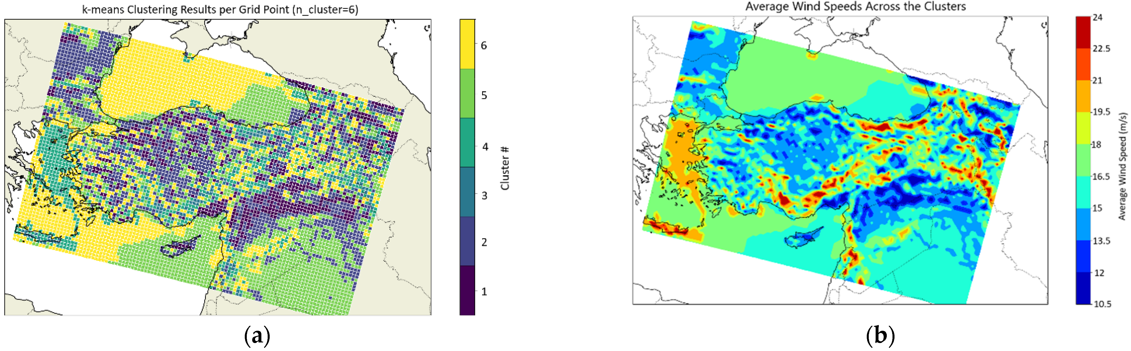
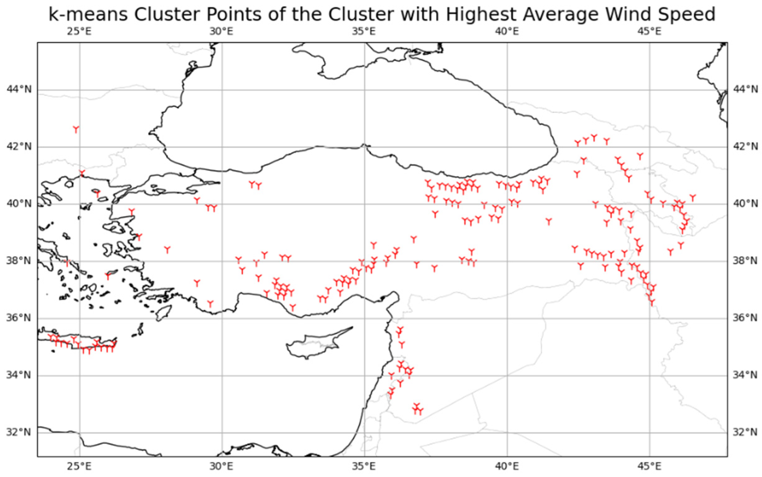
3.1. k-Means Clustering Results

The k-means clustering successfully characterized the wind dispersion patterns in the Aegean Region, considering the influence of the terrain. Nevertheless, the impact of the Black Sea and Mediterranean Region Mountain ranges on Central Anatolia was adequately represented by the k-means clustering algorithm with a 6-cluster test (Figure 7a). Also, the average values of all clusters were illustrated in Figure 7b. The resulting graph was used to highlight the cluster grid points in terms of contour plots.

Upon examination of the locations where these six clusters are created, it becomes evident that one of the patterns emerges along the Taurus Mountain ranges, which extend in an east-west direction in the southern part of the country and in the northeastern part of the area along the Black Sea coast. The Taurus Mountains and the Black Sea Mountains are both situated in parallel to the sea. A contiguous arrangement of clusters may be observed along a linear trajectory spanning from the Eastern Mediterranean to the Eastern Black Sea. A distinct pattern has emerged along a linear trajectory extending from the Black Sea Region to the eastern part of Marmara. An alternative cluster arrangement is evident, originating from the Central Black Sea Region and extending to the southern part of Central Anatolia. Comparable characteristics are also observed in the inner Aegean region. Another recurring pattern is observed throughout the Aegean coast. The Mediterranean and Black Sea exhibit distinct structural characteristics. It is clear from looking at the various clustering setups that the terrain affects the surface patterns.

3.2. EOF Analysis and SOM Clustering Results

The experiments conducted for upper-level cluster analysis were examined with a different approach. The EOF analysis was independently applied to the min-max normalized datasets for the purpose of dimensional reduction. The application of EOF to each variable is done separately to prevent the possible problem of one variable’s magnitude overpowering the combined EOF analysis as a result of the variations in units or variability. Additionally, Figure 8 displays the findings of the first three EOFs, illustrating the presence of different patterns.

On the other hand, in typical circumstances, EOF results are used to discern the main patterns of variability in upper-level data, particularly in the identification of synoptic patterns. GPH, a measure of the actual height of a pressure level in the atmosphere, is essential for comprehending synoptic weather patterns. An EOF examination of GPH at the 500 hPa level may identify prevailing wave patterns, such as ridges and troughs, which govern the movement of weather systems [59]. The following EOF modes could show secondary patterns, such as localized weather occurrences or smaller-scale characteristics. Less dominant but still significant patterns, such as a cutoff low, which can be associated with strong winds and stormy conditions, can be detected via the third EOF mode. Furthermore, MSLP, which plays a crucial role in explaining surface meteorological conditions, displays influence over wind patterns, storm courses, and frontal systems [60]. The first EOF mode often aligns with the principal synoptic pattern, including factors such as the location and intensity of high and low-pressure systems. Successive EOF modes might potentially detect additional characteristics, such as frontal systems, pressure gradients, or localized pressure anomalies. More localized pressure anomalies that drive mesoscale wind events, which can be particularly extreme, can be captured by the third EOF mode. In addition, EOF analysis can detect significant temperature anomaly patterns linked to occurrences like heatwaves, cold spells, or the location of air masses in the temperature study [61]. The initial EOF mode can uncover large-scale temperature variations, such as the distribution of warm and cold air masses or the existence of temperature anomalies. Sequential EOF modes have the potential to capture smaller-scale temperature fluctuations, such as boundaries between air masses or differences in temperature inside specific areas.

The illustration of the first EOFs of each synoptic variable explains the largest fraction of the variance in the dataset. The three leading EOFs of the data, as shown in Figure 8, account for 70.5%, 63.95%, and 58.94% of the total variance for the MSLP, Z500, and T850 variables, respectively. In Figure 8, the initial EOFs of GPH and T, which collectively account for 27% of the variance, along with the first EOF of MSLP, which accounts for 35% of the variance, are likely the most significant synoptic-scale patterns for the region. The majority of the EOF1 MSLP visuals exhibit a dominant pattern, which is consistently observed across the whole region encompassing Türkiye, the Mediterranean, and western Italy. The areas indicated by positive values in the figure, which show an opposite pattern, are also visible in the northern part of the Caspian Sea and the Gulf of Basra. The EOF1 GPH exhibits a pronounced gradient in Türkiye, which arises from differing values in the East Anatolia region compared to the northwestern part of Europe. This scenario depicts strong winds, particularly in the western areas. In Türkiye, the EOF1 T exhibits a prominent pattern at its center.

The second EOFs, which consist of 24% GPH, 19% MSLP, and 21% T, represent secondary yet significant patterns. The EOF2 MSLP exhibits pronounced gradients in Türkiye, with opposite values in northern and northeastern Europe and in Mediterranean and northern Africa. The EOF2 GPH is characterized by a unique pattern centered over Greece and Italy, and a contrasting pattern in Arabia. Türkiye is located within a strong gradient that originates from the west. A significant temperature gradient is developing over Türkiye in EOF2 T due to the positive influence of different patterns in Europe and Arabia. These variations may be attributed to the irregularities in the placement of the ridges and troughs (GPH), the distinct pressure centers (MSLP), and the related thermal gradients (T). The interaction of these patterns can result in fluctuations in both the speed and direction of wind, which can give rise to rare cases of extreme wind events.

The third EOFs, which consist of GPH with an explained variance (EV) of 12%, MSLP with an EV of 17%, and T with an EV of 11%, are most likely to represent the less persistent, more localized, or transitional characteristics of the atmospheric state. A strong gradient is observed in MSLP over Türkiye, which can be attributed to distinct atmospheric patterns present across Europe, East Africa, and Arabia. Similarly, in the EOF3 GPH analysis, a strong gradient was observed along the west-east axis across Türkiye.

Figure 8 illustrates those different patterns at the Z500, MSLP, and T850 levels in the north-west, south-east, north-east, and south-west regions of Türkiye, which contribute to the formation of a strong gradient area across the country.

In synoptic climatology, EOFs decompose a dataset into orthogonal (independent) modes of variability, which helps in understanding the spatial patterns and their temporal evolution. However, SOMs are considered as a complementary tool to classify large-scale atmospheric patterns, like those represented by the selected PCs from EOF analysis. The SOM arranges many synoptic scenarios into a grid, such as a 3 × 3 grid in our empirical setup. Each node in the grid indicates either a typical pattern or a group of similar patterns. The utilization of this grid arrangement enables a straightforward and precise representation and examination of intricate atmospheric dynamics. EOFs/PCs and SOMs together offer a potent toolkit for recognizing, categorizing, and displaying atmospheric patterns in synoptic climatology. EOFs provide a linear and orthogonal breakdown of the data, but SOMs offer a non-linear and more adaptable approach to classify and analyze the data. SOMs can capture intricate and nuanced correlations in the data, beyond the limitations of EOF which impose orthogonality constraints on the patterns. The Principal Components (PCs) generated from the EOF analysis are used as input for the SOM. This ensures that the SOM training is concentrated on the most important patterns of variability discovered by the EOF analysis so that SOM helps in interpreting large-scale drivers of local climate variability and is a part of statistical downscaling methodologies [62].

Once the SOM cluster analysis was completed, the days that belong to each SOM node, referred as SOM neurons, were extracted. Each SOM node was visualized based on the mean GPH, MSLP, and T as contour plots together (Figure 9, Figure 10, Figure 11, Figure 12 and Figure 13). A comprehensive analysis was conducted to see how these nodes may accurately represent the cumulative variability observed in the EOFs. This section primarily examines how the SOM nodes can exhibit different synoptic-scale characteristics that may impact extreme surface winds.

• SOM Node (C1): Upon analyzing the MSLP pattern, it is observed that a low-pressure system originating from Iceland forms over the Tyrrhenian Sea, west of Italy. This system influences the western and northwestern regions of Türkiye. Simultaneously, a high-pressure area centered on Iran extends from the eastern regions of Türkiye to the western part of Central Anatolia, impacting this area. The presence of two distinct pressure patterns, one spreading westward and the other eastward, results in a region where southerly and southwesterly winds dominate over Türkiye. As a result of the strong pressure gradient, areas with extreme winds are formed, particularly in the western Mediterranean, Aegean, Marmara, and Western Karadeniz regions. Within the Central and Eastern Black Sea region, the intensification of the gradient results in the formation of strong wind zones caused by westerly flows along these coastal areas. Corroborating this, there exists a significant temperature gradient at the 850 hPa level. The upper-level wave pattern shows that, the upper-level trough, linked to the low-pressure center over Italy, extends its influence on the western coasts of Türkiye. These regions are situated within the ascending flow area of the trough, resulting in a stronger impact on increasing the winds in this area. The ridge area exerts its effect over the eastern and southeastern areas. This refers to the decreased frequency of windy days in this area. The southerly airflow originating from the Mediterranean exerts an important accelerating influence, particularly on the southwestern Aegean and western Mediterranean. This dominant southerly flow pattern aligns with the high frequency of strong winds experienced, particularly in the western and northwestern regions of Türkiye. Generally, there exists a significant relationship between the frequency of days with high wind speeds and the strong pressure and temperature gradients generated by various ground-level pressure systems (Figure 9a).
• SOM Node (C2): Observations indicate that a dynamic low-pressure system, originating from Iceland, has extended its area of influence towards southern Europe. There is a thermal high-pressure system located in the eastern region of Türkiye. The prevailing wind direction in Türkiye is generally from the southwest, while westerly winds are noted around the Central Black Sea coast and the Eastern Black Sea region. The southeastern region of Türkiye experiences easterly winds because of the influence of the thermal high-pressure system. The strong pressure gradient observed in the western and northwestern areas, as well as along the Black Sea coast, correlates with the high number of days characterized by extreme winds in these specific locations. The strong temperature gradient at the 850 hPa level along the Eastern Black Sea coast also influences the number of days with high winds in this area. Similarly, when analyzing the wave pattern at higher altitudes, a strong gradient in geopotential height is observed over the western and northwestern parts of Türkiye. This, in turn, leads to a strong zonal flow at the 500 hPa level, which has a direct impact on the increase of surface winds. (Figure 9b).

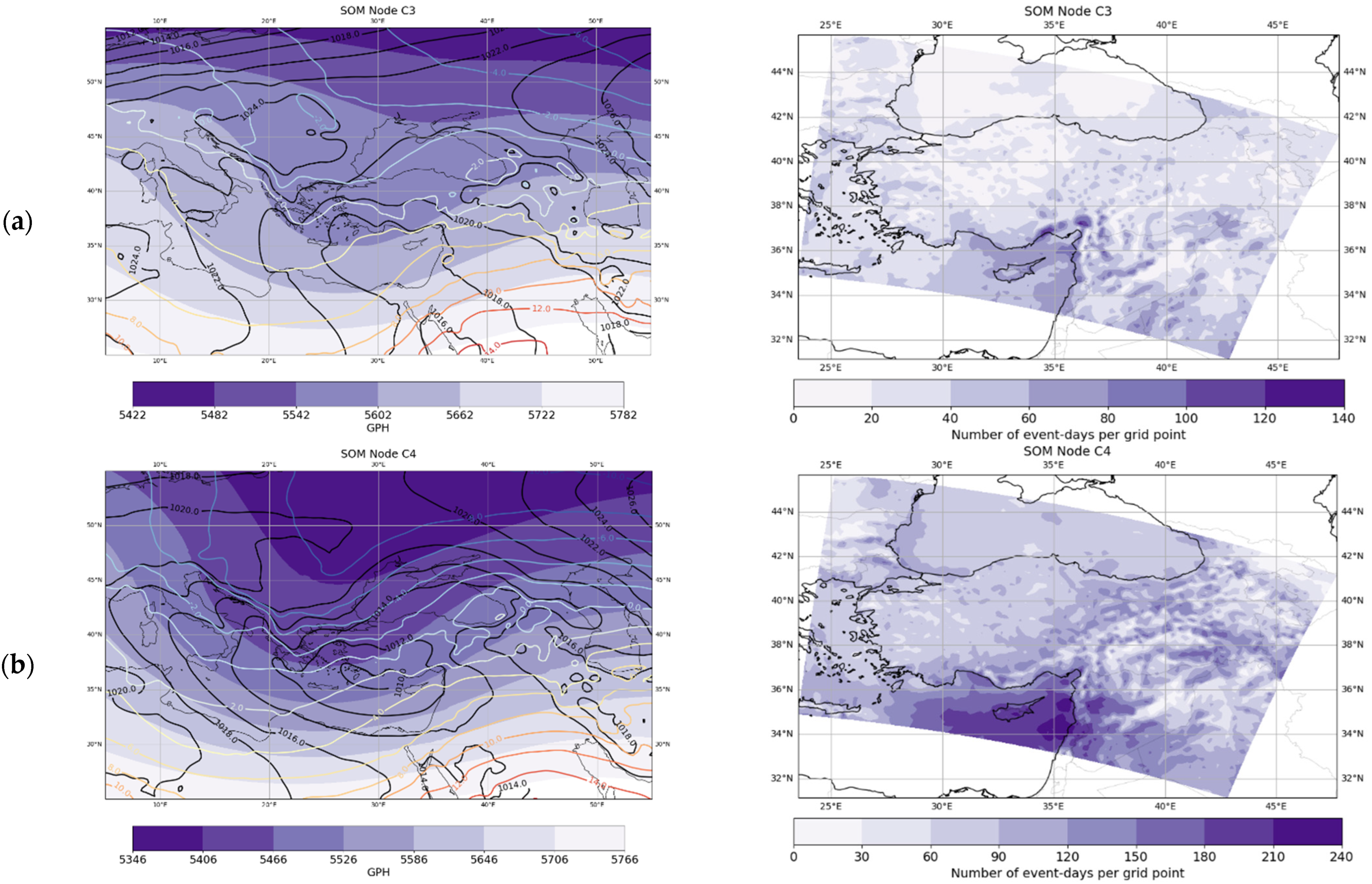
• SOM Node (C3): A high-pressure center is located over the cold central European continent. Furthermore, there exists a cold-origin Siberian high-pressure center located on the east of the Caspian Sea. The low-pressure system centered on the Red Sea affects Türkiye. The relationship between the high-pressure system situated over Europe and the low-pressure system over the Red Sea is linked to the number of days with extreme winds over the Aegean region. The temperature field at 850 hPa shows that the temperature gradient in the eastern Mediterranean region aligns with the pressure gradient at the surface level. The impact of the trough on Türkiye is observed at the 500 hPa level. The central and eastern Mediterranean Region, characterized by significant pressure and temperature gradients, is within the region of ascending flow. This accounts for the increased number of days characterized by high winds in the area (Figure 10a).
• SOM Node (C4): It is observed in this pattern that Türkiye is being affected by a low-pressure center originating from the Mediterranean, with its center located in the eastern Mediterranean region. The pressure gradient is strong in the northwestern region of Türkiye and the eastern Mediterranean. Over Türkiye, a strong temperature gradient is seen at the 850 hPa level. The upper-level wave trough is situated to the west of the ground-based low-pressure center in this pattern, which illustrates the highly baroclinic unstable structure of a frontal system over the area. The number of days with high winds along the central and eastern Mediterranean coast is influenced by the rising flow impact of the upper-level trough moving in a south-west to north-east direction (Figure 10b).

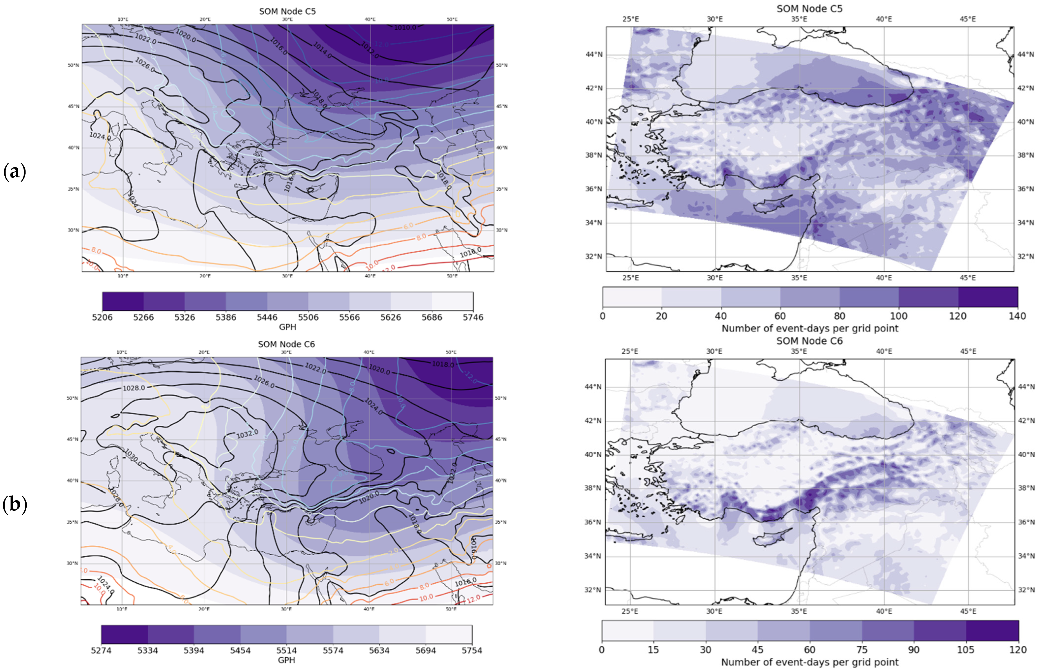
• SOM Node (C5): The Azores-originating high-pressure center exerts its influence over a broad region encompassing Türkiye, as well as western and central Europe. A low-pressure center is situated above Cyprus. The impact of a cold low-pressure system originating from Iceland extends into the northeastern region of the Black Sea in Eastern Europe. It is seen that a strong pressure and temperature gradient formed along Türkiye’s Mediterranean coast in a west-east direction when combined with an examination of the temperature at 850 hPa and the pressure at ground level. Hence, it may be asserted that a frontal system is effective in the area. Also, it is seen that there is a pressure gradient throughout the eastern Black Sea. Examining the 500 hPa wave pattern reveals that the trough connected to a cold-originating low-pressure system over Eastern Europe has extended its impact to Türkiye. The Black Sea region is within the expanding zone of the trough’s flow. The convergence of various ground and upper-level patterns is linked to areas characterized by a significant frequency of days with extreme winds (Figure 11a).
• SOM Node (C6): This node shows similar patterns with the C5 node. However, at this point, it is observed that the Azores high-pressure center has a more stable form and extends its range of influence to northern Europe. The flow pattern over Türkiye, which was predominantly northwestern and western in the preceding pattern, is therefore classified as northern in this instance. Both the ground-level pressure field and the 850 hPa level temperature field show strong pressure and temperature gradients in areas where the number of extreme windy days in this pattern is high. When looking at the geopotential height values, it becomes evident that the high-pressure area over Europe corresponds to a ridge that impacts the western part of Türkiye. Meanwhile, the middle and eastern portions of Türkiye are influenced by a trough. The trough is mostly affecting the Mediterranean and Southeastern Anatolia regions, since they are located inside its ascending flow area (Figure 11b).

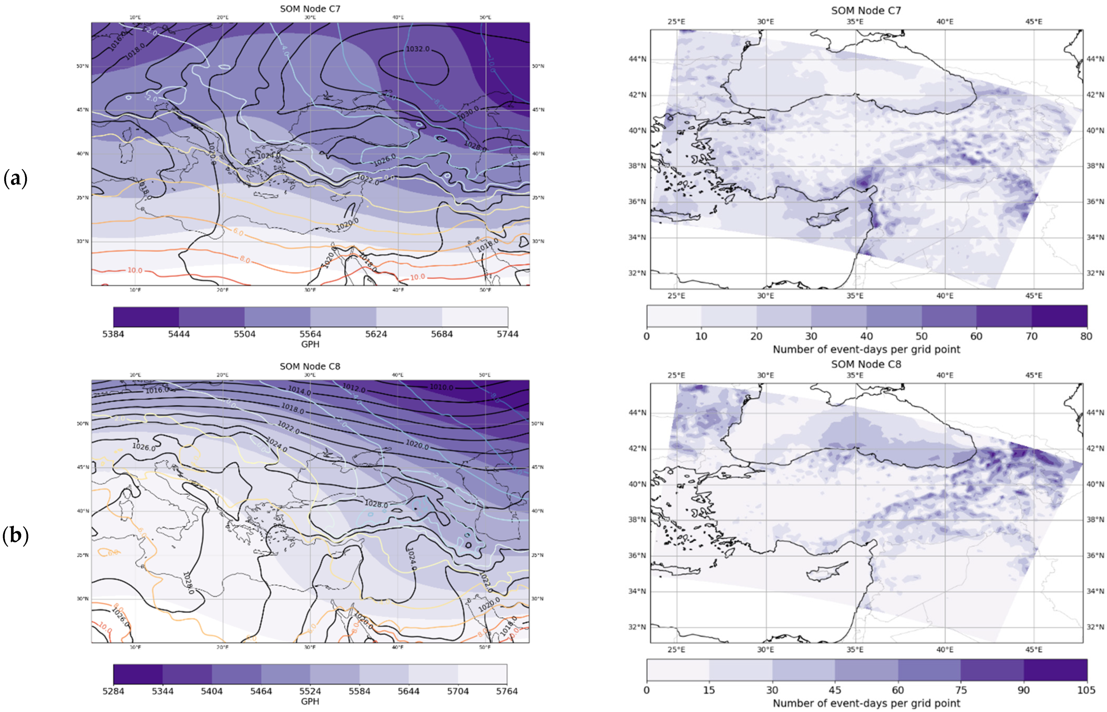
• SOM Node (C7): As the low-pressure center affects northern Europe and the Western Mediterranean, the high-pressure center originating from Siberia is observed to extend its sphere of effect towards eastern and central Europe. While Türkiye has predominantly high atmospheric pressure, there is a localized region of modest low pressure over the Eastern Black Sea. The MSLP and 850 hPa temperature indicate the presence of a strong gradient aligned in the west-east direction, running parallel to the shoreline in the Mediterranean area. Consistent with this arrangement, the number of days with strong winds is greater along this trajectory. The occurrence of extreme winds, particularly in the eastern part of the Marmara Sea and the Inner Aegean Region, may be attributed to two factors: the presence of a low-pressure system near the surface, which creates a restricted track into the Black Sea, and the temperature gradient at the 850 hpa level. The upper-level wave pattern typically exhibits a ridge effect in regions that encompass Türkiye (Figure 12a).
• SOM Node (C8): This pattern involves the influence of a high-pressure center that originates from the Azores and its accompanying ridge at the 500 hPa level. It impacts a large area encompassing central Europe, Türkiye, and northern Africa. The western areas of Türkiye are situated in a col, whereas the Anatolian plateau experiences a high-pressure center. A low-pressure system, which originated from Iceland, together with its associated 500 hPa trough, is now observable across eastern and northern Europe. The locations that have a high number of days with strong winds are found to be consistent with areas with strong pressure and temperature gradients, particularly those that stretch from the central Mediterranean to the southwest-northeast direction. Similarly, there exists a gradient of pressure over the central region, the Black Sea, and Georgia. (Figure 12b).

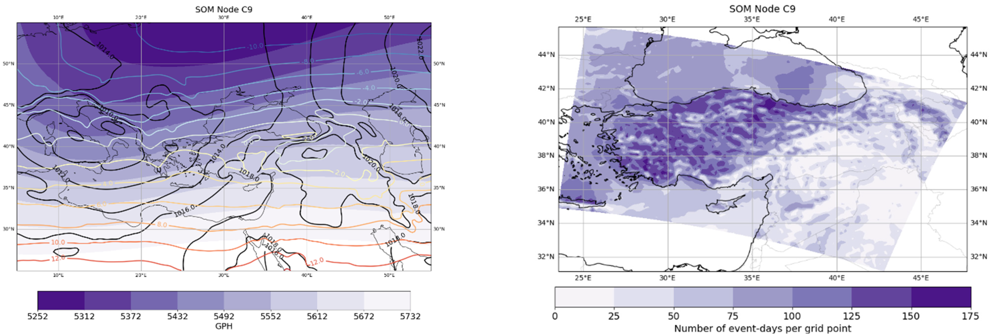
• SOM Node (C9): The Mediterranean origin low-pressure center, which is centered over Italy, is shown to have strong southern flows that affect a large portion of Türkiye. A regional high-pressure center is present in the southeastern part of Türkiye, while a low-pressure center is located over the Caspian Sea. On the low-pressure center at ground level, there is a trough at 500 hPa, but it gives way to a ridge toward Türkiye’s east. There exists a strong pressure gradient at ground level in Türkiye, apart from the southeastern area. Particularly during periods when a low-pressure system dominates Türkiye, with prevailing winds originating from the southwest and south Mediterranean, there are strong upward movements associated with the low-pressure system. Additionally, southerly winds over the open sea intensify the flow, resulting in generally strong winds observed throughout Türkiye when this weather pattern is in effect. As seen by the observed pattern, there is a rising trend in the number of days characterized by extreme winds. Nevertheless, it is observed that the southeastern area has a limited number of days characterized by extreme winds due to the dominance of high pressure (Figure 13).

The significant pressure gradients appear to create regions of strong winds throughout Türkiye. The occurrence of low-pressure and high-pressure areas, namely in the Mediterranean and the Black Sea, coupled with the corresponding frontal systems, greatly impact the frequency of days marked by extreme winds. Furthermore, the Low-Pressure Centre, primarily located over the Black Sea, exerts a significant impact on wind intensification due to its frontal effect in the area. Lastly, the Azores and Siberia, places known for their high-pressure systems, play a significant role in creating substantial gradients over Türkiye. These gradients are essential for the development of extreme winds. To summarize, it has been observed that most of the SOM nodes were representative enough to identify the common pressure systems which are effective throughout Türkiye during the winter period. Moreover, the vast majority of the extreme wind events were explained by the SOM nodes.

3.3. Relation between k-means Clustering and SOM Clustering Results

Another key point of this work is to figure out the correlation between SOM nodes and the clustering outcomes at the lower level, which is crucial in describing extreme wind events at lower level. Within this framework, a basic set of statistical data that includes the event days for each SOM node and the outcomes of clustering at a lower level was extracted. For this analysis, the k-means cluster with the highest mean speed was chosen. The rationale behind this decision assumed that the cluster exhibiting the highest average speed would have the highest correlation with SOM patterns. Based on the k-means clustering results, the mean wind speed of the grid points within the cluster aligns with this definition. The grid locations and extreme wind days are derived from data collected at 100 m a.g.l. The chosen grid points are mostly located in elevated regions of Türkiye and the Crete Island region (Figure 14).

The relation between the SOM clustering results and k-means clustering results were examined in terms of statistics. At this stage, three different statistical data were obtained. Among k-means clusters, the cluster with the highest average wind speed was identified and the grid points that belong to that cluster were determined. For each grid point, the event-days (days when at least one extreme wind speed event was simulated) were extracted. Similarly, for each SOM node, the days belonging to that node were also extracted and the number of days that belonged to that SOM node were identified by Total Event Day Count. The days in the k-means cluster with high wind speeds were related to the days assigned to each SOM node by counting the matches. Any event day having multiple events was counted as one. The total count was calculated for each grid point and the average of all grid points was recorded for each SOM node. Next, the matching event-day count for each SOM node was divided by the Total Event-Day Count for the corresponding SOM node and the Mean Event-Day Percentage was obtained. The Mean Wind Speed was also calculated in the same manner by averaging the matching event-day mean wind speeds for each SOM node. Statistical data presented in

Table 1. Lower-level k-means clustering grid points for the cluster with the highest average wind speed and upper-level SOM nodes correlation in terms of Total Event-Day Count, Mean Event-Day Percentage, and Mean Wind Speed.

	C1	C2	C3	C4	C5	C6	C7	C8	C9
Total Event-Day Count	270	311	371	433	290	199	311	224	298
Mean Event-Day Percentage	8.29%	6.76%	4.44%	10.11%	12.37%	10.33%	2.33%	5.41%	15.47%
Mean Wind Speed	22.81	21.82	22.65	22.54	22.53	23.72	22.38	22.64	22.50

provide insights into the frequency of these events and their distribution across various wind speed patterns identified by the SOM.

The statistical analysis results (Table 1) showed that the Total Event-Day Count, which represents the overall number of days with intense wind events, differed among SOM nodes. Node C9 had the highest count of 298 days. Surprisingly, this node also showed the highest Mean Event-Day Percentage (15.47%), suggesting a higher occurrence of intense wind events under its synoptic conditions compared to other nodes. The average wind speeds, although relatively consistent, exhibited a marginal increase in intensity at the C6 node, measuring 23.72 m/s.

Significant pressure and temperature gradients at the SOM node C4 indicate a low-pressure system, strong pressure and temperature gradients which are strongly correlated with the k-means high wind speed cluster. This node had a Total Event-Day Count of 433 days and a Mean Event-Day Percentage of 10.11%, which was higher than usual. This suggests that it had a significant impact on extreme wind events.

Furthermore, there is a noteworthy correlation between high wind velocities and the SOM node C5, as evidenced by its Mean Event-Day Percentage of 12.37%. The SOM node C6 shows a strong link with the highest recorded Mean Wind Speed of 23.72 m/s. This indicates that the synoptic patterns represented by this node are likely to generate the most severe wind occurrences compared to the other nodes investigated.

In summary, extreme wind events are highly frequent, and their correlation with certain SOM nodes indicates that large-scale atmospheric conditions impact regional wind patterns.

4. Conclusions

In this study, the relationship between the ground-level wind speeds and the upper-level parameters was investigated. The main objective was to accurately characterize the extreme wind conditions during the wintertime in Türkiye and examine their correlation with synoptic patterns. Cluster analysis techniques were employed to identify the correlation between them.

Two distinct atmospheric levels—the upper level and the ground level—were considered during the calculations. The lower-level data used in the first section of the analysis was taken from the NEWA dataset, which includes 48 samples daily at 6732 grid points over a 30-year period at 100 m. The 98th percentile of the data was obtained for each grid point, and these extracted values were considered as the extreme values for that grid point. The k-means clustering algorithm was utilized to classify the given datasets. After doing a k-means clustering analysis, six clusters were identified. These clusters show key patterns along the Taurus and Black Sea mountains, demonstrating the importance of topography in meteorology. The complicated connection between terrain and wind patterns is shown by the linear trajectories of clusters from the Eastern Mediterranean to the Eastern Black Sea and from the Black Sea Region to Eastern Marmara, as well as comparable patterns in the Central Black Sea and inner Aegean. These findings give a sophisticated picture of regional wind dynamics, enabling meteorological and environmental investigations in the area. Also, it was discovered that the clustering results match the widespread presence of high or strong winds throughout Türkiye. Moreover, the analysis of the dataset revealed that the winter season in the study area exhibits the most frequent occurrence of windy conditions characterized by high wind velocities.

The second phase of the study consisted of using upper-level datasets to investigate synoptic patterns. The analysis was performed using the MSLP, Z500, and T850 datasets. The data source for this analysis was the ERA5 Reanalysis data, covering DJF of a 30-year period (1998–2018). The combined application of EOF and SOM provided a detailed and multifaceted view of the atmospheric dynamics affecting Türkiye, particularly in terms of synoptic-scale wind patterns. The EOF technique was individually applied to the datasets to reduce their dimensionality while preserving the variance. The scree test indicated that the eight Z500, MSLP, and nine T850 EOFs gathered were considered adequate. Furthermore, the initial three findings of the EOF analysis were presented just to demonstrate the presence of different patterns.

The SOM technique was implemented on the MSLP, T850, and Z500 datasets, which were obtained from the EOF results. A total of nine SOM nodes were generated, following a structured grid arrangement with dimensions of 3 × 3. Each node is assigned a unique set of days for a given atmospheric state. Three primary patterns were identified for the winter season because of these analyses, despite some variations among them. The first pattern is seen to be particularly efficient in patterns with low-pressure centers located over the Mediterranean region or Italy and extending towards Türkiye. These patterns have a significant impact on Türkiye, particularly in the southern regions. Over the open sea, southern flows have the tendency to accelerate. The existence of a temperature gradient at the 850 hPa level in the relevant region, along with the ascending flow zone of the 500 hPa trough, indicates the effect of the frontal system in this area. Furthermore, the presence of these patterns in the low-pressure center in the west and the high-pressure center in the east results in strong pressure gradients throughout a broad region of Türkiye. Consequently, extreme winds are experienced during the period when these patterns are active. Examples of this pattern include nodes C1, C2, C7, and C9. A secondary dominant pattern is evident over Türkiye and the southern Mediterranean region, encompassing Cyprus. This pattern is characterized by the presence of a low-pressure center originating from the Mediterranean and an upper-level 500 hPa wave trough. Additionally, a frontal system with a temperature gradient at the 850 hPa level affects the region. The flow pattern described has a stimulating impact on the western areas of Türkiye, particularly when combined with the north-eastern winds flowing over the Black Sea. Similarly, in the Mediterranean region, the movement is intensified by winds blowing from the south. When these patterns are successful, there is an increase in the number of days with extreme winds in Türkiye. This pattern was detected at node C4. In the last pattern, the occurrence of windy days in regions with a high-pressure center over central Europe and a low-pressure center over East Africa, Asia, or Russia might be attributed to the significant pressure and temperature gradients in these locations. Illustrative nodes are C3, C6, C5, and C8. Additionally, it has been observed that the initial three EOF outcomes effectively illustrate the variations in patterns that were gathered from the SOM calculations.

The rise in elevation observed when moving from the coastal regions to the inland sections of Türkiye, particularly during winter, is a contributing element to the disparity in heating between the sea and the land. Examining temperature gradients across all SOM nodes reveals that synoptic and large-scale patterns also reflect disparities in land and sea warming, particularly at the 850 hPa level over the Mediterranean. These variations are attributed to synoptic and large-scale patterns. This phenomenon is also observed in SOM nodes C2, C5, C6, C7, and C8. Temperature differences between the sea and land on the Black Sea coast are found in SOM nodes C1 and C2. Pattern C4 is characterized by a low-pressure center and its related frontal system, which exerts influence throughout the entirety of Türkiye. The pattern demonstrates the impact of significant temperature variations throughout the whole region of Türkiye. Temperature gradients, particularly those running parallel to coasts, are a result of the significant temperature difference between the sea and land.

As a follow-up study, the days for each SOM node are identified, and the NEWA dataset is used to calculate extreme wind event frequency for each NEWA grid point. Frequency analysis reveals the association between SOM node climate conditions and extreme wind events. It has been found that some SOM clusters effectively represent the known patterns of the research region. However, several clusters within the SOM did not accurately depict the expected trends during the DJF period.

In addition, significant pressure gradients seem to produce extreme wind zones across Türkiye during the DJF period. The presence of low-pressure and high-pressure zones, namely in the Mediterranean and the Black Sea, along with the associated frontal systems, significantly influences the frequency of days characterized by extreme winds. Moreover, the Low-Pressure Center, predominantly situated above the Black Sea, exerts a substantial influence on the strengthening of winds as a result of its frontal effect in the region. Finally, the Azores and Siberia, renowned for their high-pressure systems, have a considerable impact on the formation of huge gradients over Türkiye. These gradients are crucial for the formation of extreme winds over Türkiye.

Furthermore, the local geography, characterized by Türkiye’s three-sided coastal location and the existence of elevated plateaus and mountains in the interior, also contributes to the amplification of these systems. The occurrence of mountain and sea winds is a localized phenomenon. The channel and valley impact of these systems, which influence the movement in hilly regions, also contribute to local acceleration or reduction at a small or regional level. The existence of mountain ranges running from west to east in the northern and southern parts of Türkiye, along with the rugged mountainous terrain in the Aegean region, leads to an acceleration of the flow of air. This acceleration is caused by the influence of the mountains, as well as the reinforcement of the airflow towards the continental interior due to the formation of channels in the mountainous areas.

In conclusion, this study also examined the correlation between the k-means and SOM clustering results. In the scope of this analysis, the relevant statistics were extracted using both clustering outcomes in terms of event-day counts at both levels and mean wind speed at lower-levels. Even SOM clustering efforts were focused on the winter period, the SOM results show similarities with the all-time k-means clustering results in terms of lower-level extreme wind events.

To gain a deeper comprehension of the correlation between k-means clustering and SOM, one might employ several statistical techniques to do computations. Furthermore, there are plans to carry out a comparable investigation for the remaining three sets of seasonal data. In addition, it would be worthy to conduct future study utilizing more precise grids or alternative data reduction approaches to enhance our findings. Lastly, future study may utilize Z500, MSLP, and T850 gradient computations to do more precise quantitative calculations. This will furthermore be beneficial for substantiating study findings and validating the correctness of the model.

References

1. Kunz, M.; Mohr, S.; Rauthe, M.; Lux, R.; Kottmeier, C. Assessment of extreme wind speeds from regional climate models—Part 1: Estimation of return values and their evaluation. Nat. Hazards Earth Syst. Sci. 2010, 10, 907–922. [Google Scholar] [CrossRef]
2. Ulbrich, U.; Leckebusch, G.C.; Pinto, J.G. Extra-tropical cyclones in the present and future climate: A review. Theor. Appl. Climatol. 2009, 96, 117–131. [Google Scholar] [CrossRef]
3. Palutikof, J.P.; Brabson, B.B.; Lister, D.H.; Adcock, S.T. A review of methods to calculate extreme wind speeds. Meteorol. Appl. 1999, 6, 119–132. [Google Scholar] [CrossRef]
4. Gong, X.; Richman, M.B. On the application of cluster analysis to growing season precipitation data in North America East of the Rockies. J. Clim. 1995, 8, 897–931. [Google Scholar] [CrossRef]
5. Wilks, D.S. Statistical Methods in the Atmospheric Sciences, 4th ed.; Elsevier: Amsterdam, The Netherlands, 2019. [Google Scholar]
6. Zhang, Z.; Li, J. Big Data Mining for Climate Change; Elsevier: Amsterdam, The Netherlands, 2020. [Google Scholar]
7. Pampuch, L.A.; Negri, R.G.; Loikith, P.C.; Bortolozo, C.A. A review on clustering methods for climatology analysis and its application over South America. Int. J. Geosci. 2023, 14, 877–894. [Google Scholar] [CrossRef]
8. Lorenz, E.N. Empirical Orthogonal Functions and Statistical Weather Prediction; Scientific Rep. 1, Statistical Forecasting Project; Massachusetts Institute of Technology Defense Document Center: Cambridge, MA, USA, 1956. [Google Scholar]
9. Ünal, Y.S.; Tan, E.; Menteş, Ş.S. Summer heat waves over western Turkey between 1965 and 2006. Theor. Appl. Climatol. 2012, 112, 339–350. [Google Scholar] [CrossRef]
10. Bierstedt, S.E.; Hünicke, B.; Zorita, E. Variability of wind direction statistics of mean and extreme wind events over the Baltic Sea region. Tellus A Dyn. Meteorol. Oceanogr. 2015, 67, 29073. [Google Scholar] [CrossRef]
11. Ludwig, F.L.; Horel, J.; Whiteman, C.D. Using EOF Analysis to Identify Important Surface Wind Patterns in Mountain Valleys. J. Appl. Meteorol. 2004, 43, 969–983. [Google Scholar] [CrossRef]
12. Farjami, H.; Hesari, A.R.E. Assessment of sea surface wind field pattern over the Caspian Sea using eof analysis. Reg. Stud. Mar. Sci. 2020, 35, 101254. [Google Scholar] [CrossRef]
13. Türkeş, M.; Tatlı, H. Use of the spectral clustering to determine coherent precipitation regions in Turkey for the period 1929–2007. Int. J. Climatol. 2010, 31, 2055–2067. [Google Scholar] [CrossRef]
14. Hartigan, J.A.; Wong, M.A. A k-means clustering algorithm. J. R. Stat. Soc. 1979, 28, 100–108. [Google Scholar]
15. Sinaga, K.P.; Yang, M.-S. Unsupervised k-means clustering algorithm. IEEE Access 2020, 8, 80716–80727. [Google Scholar] [CrossRef]
16. Peña, J.C.; Aran, M.; Cunillera, J.; Amaro, J. Atmospheric circulation patterns associated with strong wind events in Catalonia. Nat. Hazards Earth Syst. Sci. 2011, 11, 145–155. [Google Scholar] [CrossRef]
17. Di Bernardino, A.; Iannarelli, A.M.; Casadio, S.; Pisacane, G.; Mevi, G.; Cacciani, M. Classification of synoptic and local-scale wind patterns using k-means clustering in a Tyrrhenian coastal area (Italy). Meteorol. Atmos. Phys. 2022, 134, 30. [Google Scholar] [CrossRef]
18. Yeşilbudak, M. Clustering analysis of multidimensional wind speed data using k-means approach. In Proceedings of the 5th International Conference on Renewable Energy and Applications, Birmingham, UK, 20–23 November 2016; pp. 961–965. [Google Scholar]
19. Burlando, M. The synoptic-scale surface wind climate regimes of the Mediterranean Sea according to the cluster Analysis of ERA-40 wind fields. Theor. Appl. Climatol. 2008, 96, 69–83. [Google Scholar] [CrossRef]
20. Leckebusch, G.C.; Weimer, A.; Pinto, J.G.; Reyers, M.; Speth, P. Extreme wind storms over Europe in present and future climate: A cluster analysis approach. Meteorol. Z. 2008, 17, 67–82. [Google Scholar] [CrossRef]
21. Kohonen, T. Self-Organizing Maps; Springer Science & Business Media: Berlin, Germany, 2001. [Google Scholar]
22. Cassano, E.; Lynch, A.; Cassano, J.; Koslow, M. Classification of synoptic patterns in the western Arctic associated with extreme events at Barrow, Alaska, USA. Clim. Res. 2006, 30, 83–97. [Google Scholar] [CrossRef]
23. Cavazos, T.; Comrie, A.C.; Liverman, D.M. Intraseasonal variability associated with wet monsoons in southeast Arizona. J. Climate 2002, 15, 2477–2490. [Google Scholar] [CrossRef]
24. Reusch, D.B.; Alley, R.B.; Hewitson, B.C. Relative performance of self-organizing maps and principal component analysis in pattern extraction from synthetic climatological data. Polar Geogr. 2005, 29, 188–212. [Google Scholar] [CrossRef]
25. Srinivasa Raju, K.; Nagesh Kumar, D. Classification of Indian meteorological stations using cluster and fuzzy cluster analysis, and Kohonen artificial neural networks. Hydrol. Res. 2007, 38, 303–314. [Google Scholar] [CrossRef]
26. Khedairia, S.; Khadir, M.T. Self-organizing map and k-means for meteorological day type identification for the region of Annaba-Algeria. In Proceedings of the 7th Computer Information Systems and Industrial Management Applications, Ostrava, Czech Republic, 26–28 June 2008; pp. 91–96. [Google Scholar]
27. Spassiani, A.C.; Mason, M.S. Application of self-organizing maps to classify the meteorological origin of wind gusts in Australia. J. Wind Eng. Ind. Aerodyn. 2021, 210, 104529. [Google Scholar] [CrossRef]
28. Zhao, W.; Hao, C.; Cao, J.; Lan, X.; Huang, Y. Characteristics of large-scale atmospheric circulation patterns conducive to severe spring and winter wind events over Beijing in China based on a machine learning categorizing method. Front. Earth Sci. 2022, 10, 998108. [Google Scholar] [CrossRef]
29. Kim, H.; Kim, B.-J.; Nam, H.-G.; Jeong, J.; Shim, J.-K.; Kim, K.R.; Kim, S. Classification of homogeneous regions of Strong wind and gust wind in Korea. SOLA 2020, 16, 140–144. [Google Scholar] [CrossRef]
30. Türkeș, M.; Yozgatlıgil, C.; Batmaz, İ.; İyigün, C.; Kartal Koç, E.; Fahmi, F.; Aslan, S. Has the Climate Been Changing in Turkey? Regional Climate Change Signals Based on a Comparative Statistical Analysis of Two Consecutive Time Periods, 1950–1980 and 1981–2010. Clim. Res. 2016, 70, 77–93. [Google Scholar] [CrossRef]
31. Kömüşcü, A.Ü.; Turgu, E.; DeLiberty, T. Dynamics of Precipitation Regions of Turkey: A Clustering Approach by K-Means Methodology in Respect of Climate Variability. J. Water Clim. Change 2022, 13, 3578–3606. [Google Scholar] [CrossRef]
32. Türkeş, M.; Erlat, E. Influences of the North Atlantic oscillation on precipitation variability and change in Turkey. Il Nuovo C. C 2005, 29, 117–135. [Google Scholar]
33. Çetin, İ.I. Potential Impacts of Climate Change on Wind Energy Resources in Turkey. Ph.D. Thesis, Middle East Technical University, Ankara, Türkiye, 2023. [Google Scholar]
34. Özen Bayraktar, S.; Çiçek, İ. Türkiye’de Hortumların Sinoptik Desen Sınıflamaları. Coğrafi Bilim. Derg. 2023, 21, 594–615. [Google Scholar] [CrossRef]
35. Tatlı, H.; Menteş, Ş.S. Detrended cross-correlation patterns between North Atlantic oscillation and precipitation. Theor. Appl. Climatol. 2019, 138, 387–397. [Google Scholar] [CrossRef]
36. Bastine, D.; Larsén, X.; Witha, B.; Dörenkämper, M.; Gottschall, J. Extreme winds in the new European wind atlas. J. Phys. Conf. Ser. 2018, 1102, 012006. [Google Scholar] [CrossRef]
37. Mann, J.; Angelou, N.; Arnqvist, J.; Callies, D.; Cantero, E.; Arroyo, R.C.; Courtney, M.; Cuxart, J.; Dellwik, E.; Gottschall, J.; et al. Complex terrain experiments in the new European wind atlas. Philos. Trans. R. Soc. A Math. Phys. Eng. Sci. 2017, 375, 20160101. [Google Scholar] [CrossRef] [PubMed]
38. Menteş, Ş.; Ünal, Y.; Ezber, Y.; Barutçu, B.; Aslan, Z.; Kirkil, G.; Topçu, S.; Erten, E.; İncecil, S.; Önol, B. Yeni Avrupa Rüzgar Atlası (NEWA) Projesi Kapsamında Türkiye Üzerine Rüzgar Enerji Kaynağının Modellenmesi; TÜBİTAK: Ankara, Turkey, 2019. [Google Scholar]
39. Martius, O.; Pfahl, S.; Chevalier, C. A Global Quantification of Compound Precipitation and Wind Extremes. Geophys. Res. Lett. 2016, 43, 7709–7717. [Google Scholar] [CrossRef]
40. Tatlı, H.; Dalfes, H.N.; Menteş, Ş.S. A statistical downscaling method for monthly total precipitation over Turkey. Int. J. Climatol. 2004, 24, 161–180. [Google Scholar] [CrossRef]
41. Hersbach, H.; Bell, B.; Berrisford, P.; Hirahara, S.; Horányi, A.; Muñoz-Sabater, J.; Nicolas, J.; Peubey, C.; Radu, R.; Schepers, D.; et al. The ERA5 global reanalysis. Q. J. R. Meteorol. Soc. 2020, 146, 1999–2049. [Google Scholar] [CrossRef]
42. Peixoto, J.P.; Oort, A.H. Physics of Climate; American Institute of Physics: Melville, NY, USA, 1992. [Google Scholar]
43. Hersbach, H.; Bell, B.; Berrisford, P.; Biavati, G.; Horányi, A.; Muñoz Sabater, J.; Nicolas, J.; Peubey, C.; Radu, R.; Rozum, I.; et al. ERA5 Hourly Data on Pressure Levels from 1940 to Present; Copernicus Climate Change Service (C3S) Climate Data Store (CDS); Available online: https://cds.climate.copernicus.eu/cdsapp#!/dataset/reanalysis-era5-pressure-levels?tab=overview (accessed on 26 November 2023).
44. Hersbach, H.; Bell, B.; Berrisford, P.; Biavati, G.; Horányi, A.; Muñoz Sabater, J.; Nicolas, J.; Peubey, C.; Radu, R.; Rozum, I.; et al. ERA5 Hourly Data on Single Levels from 1940 to Present; Copernicus Climate Change Service (C3S) Climate Data Store (CDS); Available online: https://cds.climate.copernicus.eu/cdsapp#!/dataset/reanalysis-era5-single-levels?tab=overview (accessed on 26 November 2023).
45. Kalnay, E.; Kanamitsu, M.; Kistler, R.; Collins, W.; Deaven, D.; Gandin, L.; Iredell, M.; Saha, S.; White, G.; Woollen, J.; et al. The NCEP/NCAR 40-year reanalysis project. Bull. Am. Meteorol. Soc. 1996, 77, 437–471. [Google Scholar] [CrossRef]
46. Holton, J.R.; Hakim, G.J. An Introduction to Dynamic Meteorology; Academic Press: Cambridge, MA, USA, 2013. [Google Scholar]
47. Wallace, J.M.; Hobbs, P.V. Atmospheric Science; Elsevier: Amsterdam, The Netherlands, 2006. [Google Scholar]
48. Dee, D.P.; Uppala, S.M.; Simmons, A.J.; Berrisford, P.; Poli, P.; Kobayashi, S.; Andrae, U.; Balmaseda, M.A.; Balsamo, G.; Bauer, P.; et al. The ERA-interim reanalysis: Configuration and performance of the data assimilation system. Q. J. R. Meteorol. Soc. 2011, 137, 553–597. [Google Scholar] [CrossRef]
49. MacQueen, J. Some methods for classification and analysis of multivariate observations. In Proceedings of the 5th Berkeley Symposium on Mathematical Statistics and Probability, Berkeley, CA, USA, 21 June 1967; Volume 1, pp. 281–297. [Google Scholar]
50. Arthur, D.; Vassilvitskii, S. K-means++: The advantages of careful seeding. In Proceedings of the Annual ACM-SIAM Symposium on Discrete Algorithms, New Orleans, LA, USA, 7–9 January 2007; pp. 1027–1035. [Google Scholar]
51. Wu, K.-L.; Yang, M.-S. Alternative C-Means Clustering Algorithms. Pattern Recognit. 2002, 35, 2267–2278. [Google Scholar] [CrossRef]
52. Milligan, G.W.; Cooper, M.C. A study of standardization of variables in cluster analysis. J. Classif. 5 1988, 181–204. [Google Scholar] [CrossRef]
53. Jain, A.K.; Murty, M.N.; Flynn, P.J. Data clustering: A review. ACM Comput. Surv. 1999, 31, 264–323. [Google Scholar] [CrossRef]
54. Kohonen, T. Self-organized formation of topologically correct feature maps. Biol. Cybern. 1982, 43, 59–69. [Google Scholar] [CrossRef]
55. Kaski, S.; Kohonen, T. Exploratory data analysis by the self-organizing map: Structures of welfare and poverty in the world. In Proceedings of the Third International Conference on Neural Networks in the Capital Markets, London, UK, 11–13 October 1995; pp. 498–507. [Google Scholar]
56. Jolliffe, I.T. Principal Component Analysis; Springer Science & Business Media: Berlin, Germany, 2013. [Google Scholar]
57. Vesanto, J.; Himberg, J.; Alhoniemi, E.; Parhankangas, J. SOM Toolbox for Matlab 5; Helsinki University of Technology, Neural Networks Research Centre: Espoo, Finland, 2000. [Google Scholar]
58. Kaski, S. Data Exploration Using Self-Organizing Maps. Ph.D. Thesis, Finnish Academy of Technology, Helsinki, Finland, 1997. [Google Scholar]
59. Qiao, S.; Zou, M.; Cheung, H.N.; Zhou, W.; Li, Q.; Feng, G.; Dong, W. Predictability of the wintertime 500 hpa geopotential height over Ural-Siberia in the NCEP climate forecast system. Clim. Dyn. 2019, 54, 1591–1606. [Google Scholar] [CrossRef]
60. Thornton, H.E.; Smith, D.M.; Scaife, A.A.; Dunstone, N.J. Seasonal predictability of the East Atlantic pattern in late autumn and early winter. Geophys. Res. Lett. 2023, 50, e2022GL100712. [Google Scholar] [CrossRef]
61. Martinez, Y.; Yu, W.; Lin, H. A new statistical–dynamical downscaling procedure based on eof analysis for regional time series generation. J. Appl. Meteorol. Climatol. 2013, 52, 935–952. [Google Scholar] [CrossRef]
62. Wolski, P.; Jack, C.; Tadross, M.; van Aardenne, L.; Lennard, C. Interannual rainfall variability and som-based circulation classification. Clim. Dyn. 2018, 50, 479–492. [Google Scholar] [CrossRef]
Figure 1. Application of grid point reduction to NEWA above ground level data (100 m a.g.l.).
Atmosphere 15 00196 g001
Figure 2. Türkiye and its surrounding regions: a topographic and geographical map (Basemap: ArcGIS World Imagery).
Atmosphere 15 00196 g002
Figure 3. The 98th percentile of averaged wind speed (ms−1) at the selected grid points at 100 m a.g.l.
Atmosphere 15 00196 g003
Figure 4. Elbow method results to determine optimum number of clusters for k-means: (a) total variance explained by the number of clusters; (b) Within-Cluster Sum of Squares (WCSS) by the number of clusters.
Atmosphere 15 00196 g004
Figure 5. The percentage of monthly events in the 98th percentile during the 30-year period (1989–2018).
Atmosphere 15 00196 g005
Figure 6. Scree tests based on the variance fractions per EOF: (a) geopotential height at 500 hPa; (b) mean sea-level pressure; (c) temperature at 850 hPa.
Atmosphere 15 00196 g006
Figure 7. Comparative visualization of k-means clustering results for six clusters. (a) Six distinct clusters, each represented by unique colors corresponding to different grid points. (b) Spatial distribution of wind speeds (ms−1) across the clusters where each grid point is characterized by its average wind speed.
Atmosphere 15 00196 g007
Figure 8. The first three Empirical Orthogonal Functions (EOFs) during DJF for a period of 30 years (1989–2018): (a) MSLP; (b) 500 hPa geopotential height; (c) 850 hPa temperature.
Atmosphere 15 00196 g008
Figure 9. Illustration of SOM (3 × 3) results on DJF period: MSLP as black contour lines, T850 as colored contour line, and Z500 as purple contours (gradients). (a) SOM node C1 and days with 98th percentile wind speeds for each grid; (b) SOM node C2 and days with 98th percentile wind speeds for each grid.
Atmosphere 15 00196 g009
Figure 10. Illustration of SOM (3 × 3) results on DJF period: MSLP as black contour lines, T850 as colored contour line, and Z500 as purple contours (gradients). (a) SOM node C3 and days with 98th percentile wind speeds for each grid; (b) SOM node C4 and days with 98th percentile wind speeds for each grid.
Atmosphere 15 00196 g010
Figure 11. Illustration of SOM (3 × 3) results on DJF period: MSLP as black contour lines, T850 as colored contour line, and Z500 as purple contours (gradients). (a) SOM node C5 and days with 98th percentile wind speeds for each grid; (b) SOM node C6 and days with 98th percentile wind speeds for each grid.
Atmosphere 15 00196 g011
Figure 12. Illustration of SOM (3 × 3) results on DJF period: MSLP as black contour lines, T850 as colored contour line, and Z500 as purple contours (gradients). (a) SOM node C7 and days with 98th percentile wind speeds for each grid; (b) SOM node C8 and days with 98th percentile wind speeds for each grid.
Atmosphere 15 00196 g012
Figure 13. Illustration of SOM (3 × 3) results on DJF period: MSLP as black contour lines, T850 as colored contour line, and Z500 as purple contours (gradients). SOM node C9 and days with 98th percentile wind speeds for each grid.
Atmosphere 15 00196 g013
Figure 14. Lower-level grid points for the cluster with the highest average wind speed based on k-means clustering results.
Atmosphere 15 00196 g014