Article

Development and Evaluation of a Short-Term Ensemble Forecasting Model on Sea Surface Wind and Waves across the Bohai and Yellow Sea

Institute of Oceanographic Instrumentation, Qilu University of Technology (Shandong Academy of Sciences), Qingdao 266001, China
*
Author to whom correspondence should be addressed.
Atmosphere 2024, 15(2), 197; https://doi.org/10.3390/atmos15020197
Submission received: 10 January 2024 / Revised: 25 January 2024 / Accepted: 2 February 2024 / Published: 4 February 2024
(This article belongs to the Special Issue The Challenge of Weather and Climate Prediction)

Abstract

:
In this study, an ensemble forecasting model for in situ wind speed and wave height was developed using the Coupled Ocean–Atmosphere–Wave–Sediment Transport (COAWST) model. This model utilized four bias correction algorithms—Model Output Statistics (MOS), Back Propagation Neural Network (BPNN), Long Short-Term Memory (LSTM) neural network, and Convolutional Neural Network (CNN)—to construct ensemble forecasts. The training data were derived from the COAWST simulations of one year and observations from three buoy stations (Laohutan, Zhifudao, and Lianyungang) in the Yellow Sea and Bohai Sea. After the optimization of the bias correction model training, the subsequent evaluations on the ensemble forecasts showed that the in situ forecasting accuracy of wind speed and wave height was significantly improved. Although there were some uncertainties on bias correction performance levels for individual algorithms, the uncertainties were greatly reduced by the ensemble forecasts. Depending on the dynamic weight assignment, the ensemble forecasts presented a stable performance even when the corrected forecasts by three algorithms had an obvious negative bias. Specifically, the ensemble forecasting bias was found with a mean reduction of about 96%~99% and 91%~95% for wind speed and wave height, and a reduction of about 91%~98% and 16%~54% during the period of Typhoon “Muifa”. For the four correction algorithms, the performance of bias correction was not directly related to the algorithm complexity. However, the strategies with more complex algorithms (i.e., CNN) were more conservative, and simple algorithms (i.e., MOS) might have induced unstable performance levels despite their lower bias in some cases.

1. Introduction

Marine weather forecasts play an important role in ship navigation, maritime operations, and disaster warnings. The prediction of sea surface winds and waves is one of the key forecasting elements that directly affect human productivity and well-being. Winds are the primary force behind wave generation in coastal regions close to the land, and the contribution of swells to wave generation there is relatively smaller. Therefore, predicting the accuracy of sea surface winds is vital for wind and wave forecasting. In contrast to other variables (temperature and atmospheric pressure), which fluctuate continuously, sea surface winds represent specific phases or abrupt changes based on their temporal fluctuations. Sudden changes in sea surface winds can further affect the sea surface waves. The limited in situ observational data on sea surface wind and waves have resulted in a lack of variability in the forecasting process [1].
In order to improve the accuracy of wind and wave forecasts on the sea surface, numerous studies have been conducted to assimilate satellites, stations, buoys, and other data into numerical forecasting. For example, Huang et al. (2020) assimilated the wind observations from the Advanced Scatterometer (ASCAT) and the Oceansat-2 Scatterometer (OSCAT) into the global ocean surface wind analysis [2]. Compared to the surface wind forecasts at 10 m levels from the European Centre for Medium-Range Weather Forecasts (ECMWF), the root mean square error (RMSE) of the assimilated forecasts decreased from 1.17 m/s to 1.07 m/s, and the mean bias decreased from −0.14 m/s to −0.08 m/s. The UK Met Office assimilated the hourly wind observations into its high-resolution operational forecasting model using the four-dimensional variational assimilation method. In the winter of 2016 and the summer of 2017, the mean bias and RMSE of the wind profile forecasts decreased by 15% and 10%. Other elements at the surface also showed improvements ranging from 0.27% to −0.71% [3]. Sannasiraj et al. [4] assimilated the wave observations from three buoys in the Arabian Sea into the Wave Model (WAM). They found that the RMSE of the wave height reduced by approximately 30% to 50%.
In addition to the data assimilation methods, empirical post-processing correction techniques have been widely used owing to their low computational expense and good effectiveness [5,6]. Traditional post-processing methods are usually parameter-based methods, which can be divided into three types. The first one is based on the principle of regression, usually in the form of Model Output Statistics (MOS) or Ensemble Model Output Statistics (EMOS) [7]. The second one is based on joint probability such as the meta-Gaussian and Bayesian joint probability model. The last one is based on kernel-density techniques such as the Bayesian model averaging (BMA) algorithm [8]. Because of its simplicity and efficacy, the MOS algorithm has been widely used in many fields. The machine learning algorithms like artificial neural networks were used subsequently instead of the traditional parameter-based methods. For example, Kunić et al. [9] proposed a new artificial neural network called “FOCUS” that corrected wind speed results from the numerical forecasts of five years for the Krk Bridge in Croatia. The results indicated that the corrected forecasts performed better than the uncorrected results during almost half of the validation period. Numerous empirical forecasting models have emerged in recent years due to the development of artificial intelligence algorithms, including deep learning algorithms with deep network structures. For example, the Huawei company developed a global forecasting model called Pangu-Weather, which has higher accuracy than the Integrated Forecast System (IFS) and FourCastNet in deterministic forecasts [10]. Artificial intelligence algorithms are also widely used in the nowcasting of extreme weather, which produce accurate clouds and precipitation forecasts [11]. For bias correction in post-processing, these deep learning models also represent a high operation potential. One typical example is the use of the Long Short-Term Memory (LSTM) algorithm by Kim et al. [12]. to correct the Madden–Julian Oscillation (MJO) predictions. The LSTM reduced the error by 90% for the MJO amplitude and by 77% for the MJO phase within four weeks.
Because of the abrupt and highly nonlinear characteristics, the forecasting accuracy of winds and waves has always been an operational challenge [13,14]. Some post-processing techniques were utilized in previous studies to improve the forecasting accuracy. For example, Han et al. used CU-net to correct the wind speed forecasts in North China. They found that it increased the forecast accuracy by 18.57% in the next 24 h and by 3.7% in the next 240 h when compared to the Anomaly Numerical-correction via Observations (ANO) algorithm [15]. Chen et al. used the ConvLSTM algorithm to correct the wind speed bias from numerical weather forecasts for ten stations in Belgium in 2019 and found that the mean absolute errors were reduced by 41.13–77.70%, and the RMSEs were reduced by 37.30–75.10% [16].
These bias correction methods based on machine learning or deep learning have been proven to achieve good forecasting performance. However, it is challenging for these empirical methods to guarantee highly accurate forecasts in all locations. Ensemble methods are commonly used in operational forecasting to reduce system errors. They involve averaging different forecasting results to obtain predictions with stronger adaptability to environmental changes and lower errors.
In the past, we developed a forecasting system using the Coupled Ocean–Atmosphere–Wave–Sediment Transport (COAWST) model [17]. It corrects the warm bias of WRF to some extent, and is suitable for simulating extreme weather such as typhoons. The system also has the capability of predicting the sea surface wind speed and wave height in a coupled way. However, the forecasting bias of the system in terms of wind and waves remains high, which has posed great challenges to practical applications. This issue was also presented by Liu et al. (2006) when they verified the forecasts of the COAWST model during typhoon periods using buoy observations [18].
In this study, based on this forecasting system, we further developed a post-processing module. This module utilized four different bias correction algorithms in different principles to correct the wind speed and wave height bias in the COAWST forecasts. These corrected forecasts were then subjected to ensemble averaging to generate forecasting products for wind speed and wave height at stations in the Yellow Sea and Bohai Sea.
The Yellow Sea and Bohai Sea are marginal seas located in the northwestern Pacific Ocean, surrounded by densely populated areas. These seas are the sites of frequent shipping, fishing, and exploration activities. Thus, it is vital to have accurate forecasts of winds and waves to protect human activities from disasters. The marine observations are much fewer than the land observations. The buoy data are some of the most important in situ observation sources, and other remote sensing observations at sea also use them for calibration. Therefore, the buoy observations can be used as a reference to correct the numerical forecasting errors rather than utilizing other data sources. Ebuchi et al. evaluated the wind data observed by the QuikSCAT/SeaWinds satellites and also used the buoy data as references [19].
The forecasting model developed in this study provided the in situ forecasts of winds and waves, using real-time monitoring data from three buoys over the Yellow Sea and Bohai Sea. This study investigated the performance levels of the four individual correction models and ensemble forecasts. In order to further evaluate the forecasting level of the model developed, the ERA5 reanalysis data were also utilized to compare with the forecasts.
The following section (Section 2) includes the model, correction algorithms, ensemble scheme, and data used in this study. Section 3 includes the design of the experiment, model configurations and operation steps. A detailed evaluation of the results is provided in Section 4. Section 5 discusses the limitations of the experimental design as well as the uncertainties in the results. Finally, Section 6 briefly summarizes this study.

2. Model, Algorithms, and Data

2.1. COAWST Model

The COAWST model was developed by Warner et al. in 2010. The model consists of several sub-models, including the Weather Research and Forecasting Model (WRF), the Regional Ocean Model System (ROMS), and the Simulating Waves Nearshore (SWAN) model. The Model Coupling Toolkit (MCT) is used to divide the grids of each model into segments and to allocate processors for processing. The MCT is then used to exchange and convert various information in parallel among the sub-models [20].
Numerous previous studies indicated the excellent performance of the COAWST model. For example, Maitane et al. [21] used COAWST to simulate the changes at the sea surface when Hurricane “Ida” passed across the Gulf of Mexico in November 2009. The validation results showed that the fully coupled model using COAWST provided the most accurate simulations of wind intensity with a skill index of 0.9. Zambon et al. [22] conducted a hindcast of the tropical cyclone “Ivan” in 2004 using COAWST. They found that COAWST corrected the cyclone’s moving track from the WRF model in a moderate level and significantly improved the forecasts of cyclone center intensity. The root mean square error (RMSE) of wave height from COAWST was 0.93 m, with a correlation coefficient of 0.97. In addition, the COAWST model also performed well in the hydro-meteorological simulations over China [23].

2.2. Bias correction Algorithms

2.2.1. Model Output Statistics (MOS)

The Model Output Statistics (MOS) algorithm was proposed by Glahn and Lowry. The principle of this approach is to establish an empirical relationship between the model outputs and the observations by polynomial fitting. Using the established relationship, the model bias can be estimated based on the forecasting results [24]. The schematic diagram of MOS is shown in Figure 1a.

2.2.2. Back Propagation Neural Network (BPNN)

The Back Propagation Neural Network (BPNN), proposed by Rumelhart and McCleland, is one of the most widely used algorithms in supervised learning [25]. BPNN can simulate the structure of the human brain while using a gradient descent approach to adjust the weights of neurons. It is known as a multi-layer feedforward network model with the error propagation algorithm as the core [26]. Its topological structure is shown in Figure 1b, which includes an input layer, a hidden layer, and an output layer. The training network continuously adjusts the weight relationship between the input data and the output data through forward propagation and backward propagation, thereby establishing a final mapping relationship.

2.2.3. Long Short-Term Memory Neural Network (LSTM)

As a type of recurrent neural network, the Long Short-Term Memory neural network (LSTM) was initially developed by Hochreiter et al. in 1997 [27]. The external structure of LSTM is shown in Figure 1c, which resembles a fully connected neural network. However, LSTM further adds neural network units in its hidden layer, and each neuron unit includes multiplication gates and forget gates. These gate units determine the type of data passing through the neural network. Its advantage in processing lengthy texts is guaranteed by the structure of the algorithm.

2.2.4. Convolutional Neural Network (CNN)

The Convolutional Neural Network (CNN) consists of an input layer, a convolutional layer and an output layer. Its main feature is local connectivity [28], which is suitable for feature extraction and obtaining image features. It has been widely used in image segmentation and image recognition fields. Since text data were used in this study, a one-dimensional Convolutional Neural Network (1-D CNN) was chosen for the following correction process. The structure of 1-D CNN is shown in Figure 1d. The 1-D CNN extracts features from samples by adjusting the size of the convolutional kernel and the direction of movement. This approach avoids the complex operations involved in constructing and processing multidimensional samples and demonstrates its superiority in processing long-term text series [29].
Essentially, the four algorithms above all utilize forecasting data and observation data during the training period to establish a mapping relationship from forecast values to observation values. Thus, during operational forecasting, this mapping relationship can be used to estimate the “true” value (observation) at that moment based on numerical forecasts. The key differences among these four algorithms mainly come from the methods or principles used to establish this mapping relationship. Specifically, the MOS algorithm establishes the relationship between forecast and observation through simple polynomial fitting. The other three algorithms, BPNN, CNN, and LSTM, all use more complex neural networks to establish the relationship, with differences in the complexity and computation of the neural network. BPNN is a classic machine learning algorithm that uses relatively few hidden layers and a fully connected neural structure. CNN is a representative algorithm of deep learning, which can be considered a more complex BPNN algorithm in a sense. It has more hidden layers and uses partially connected neural structures to enhance local perceptual learning. LSTM is also a deep learning algorithm, and its biggest difference from BPNN and CNN is that it uses time recursion during the training process. This allows it to bring back information from the later part as “memory” to assist in model training for the earlier part.

2.3. Ensemble Mean Method

Based on the concept of ensemble forecasting, the developed model in this study utilized a simple ensemble method of weighted bias removal to average four bias-corrected forecasting results. This ensemble method focused on reducing the mean bias of the forecasts by utilizing in situ buoy data from the previous day to calculate dynamically changing weights over time. Thus, the ensemble forecasting value M can be expressed as:
M e n s , d t = O d 1 ¯ + i = 1 N α i , d ( M i , d t M i , d 1 ¯ )
where Mens,dt represents the forecasts at the time t on the day d; Od−1 represents the buoy observation on the day d − 1; i is the id of bias-corrected forecasts; N is the number of forecasts, and here it is 4; αi,d represents the weight for the forecast Mi on the day d, which can be calculated by the RMSE of Mi on the day d − 1:
α i , d = E i , d 1 i = 1 N E I , d 1
and E is defined as the reciprocal of RMSE within the 24 H of one day:
E = R M S E 1 = 24 j = 1 24 ( M j O j ) 2
If the RMSE is zero during the calculation, it will convert to a small number (i.e., 1 × 10⁻¹²).
In this study, this ensemble mean method was designed to reduce the uncertainty caused by single bias correction algorithm. For one specific correction algorithm, it could not guarantee minimum bias in all cases, and thus, the ensemble mean method could adjust model weights to mitigate the negative effects on final forecasting results when a certain algorithm produced significant bias. Weight adjustment mainly depended on the RMSEs of the four groups of corrected forecasts in the previous day. If an algorithm had low bias in the previous day, it would receive a higher weight on the current day. Furthermore, the RMSE statistics was chosen from the previous 24 h instead of shorter time ahead, because the low real-time buoy data were updated once a day on the website.

2.4. Operational Flowchart of Forecasting System

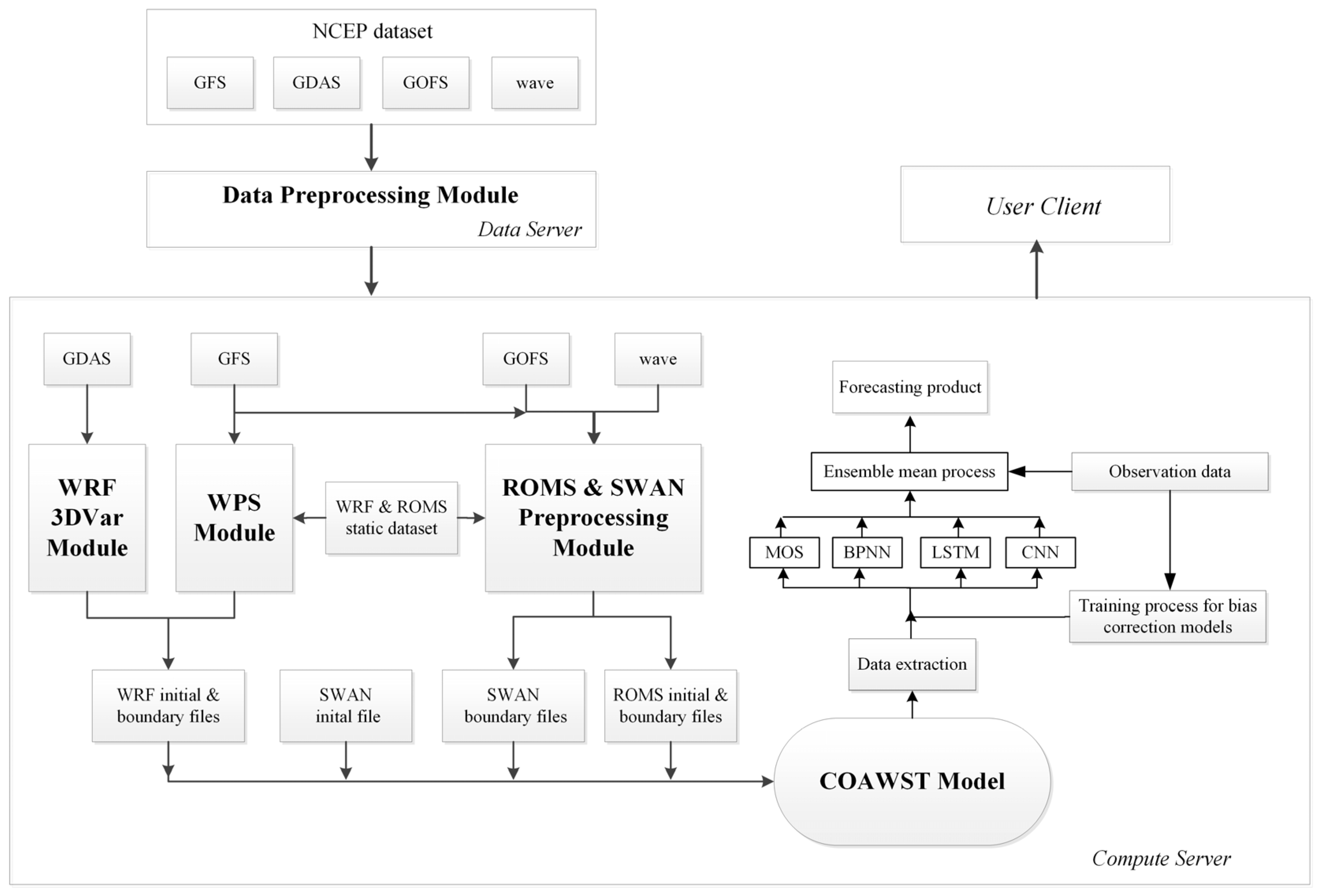
The flowchart of forecasting system is shown in Figure 2.
The driving data for WRF sub-model were derived from the Global Forecast System (GFS, available online at https://www.ncei.noaa.gov/products/ (accessed on 3 February 2024)). The driving data for ROMS sub-model were derived from the Global Ocean Forecasting System (GOFS, available online at https://www.geo-fs.com/ (accessed on 3 February 2024)) of the Hybrid Coordinate Oceanic Circulation Model (HYCOM) model. The driving data for SWAN sub-model were derived from the GFS_wave dataset. The data from Global Data Assimilation System (GDAS, available online at https://www.ncei.noaa.gov/data/ncep-global-data-assimilation/access/ (accessed on 3 February 2024)) were also derived for the assimilation module in the WRF sub-model. For the initial and boundary conditions of the models, WRF, ROMS, and SWAN all used default cold starting ways for initialization.
Using the initial conditions and boundary files from the three sub-models, the COAWST model was run and generated forecasting results for the next 72 h. The forecasted variables at sea surface were then extracted to construct four bias correction models (MOS, BPNN, LSTM, and CNN). Prior to model training, multiple groups of sensitivity tests were conducted to optimize the bias correction models (detailed steps are described in Section 3.2) for more accurate forecasting bias estimation. The trained bias correction models took forecasted sea-surface variables as inputs and output bias-corrected predictions of surface wind speed and wave height. These forecasting results were then subjected to ensemble averaging to produce forecast products at station locations for display and use in user clients.

2.5. Data Description

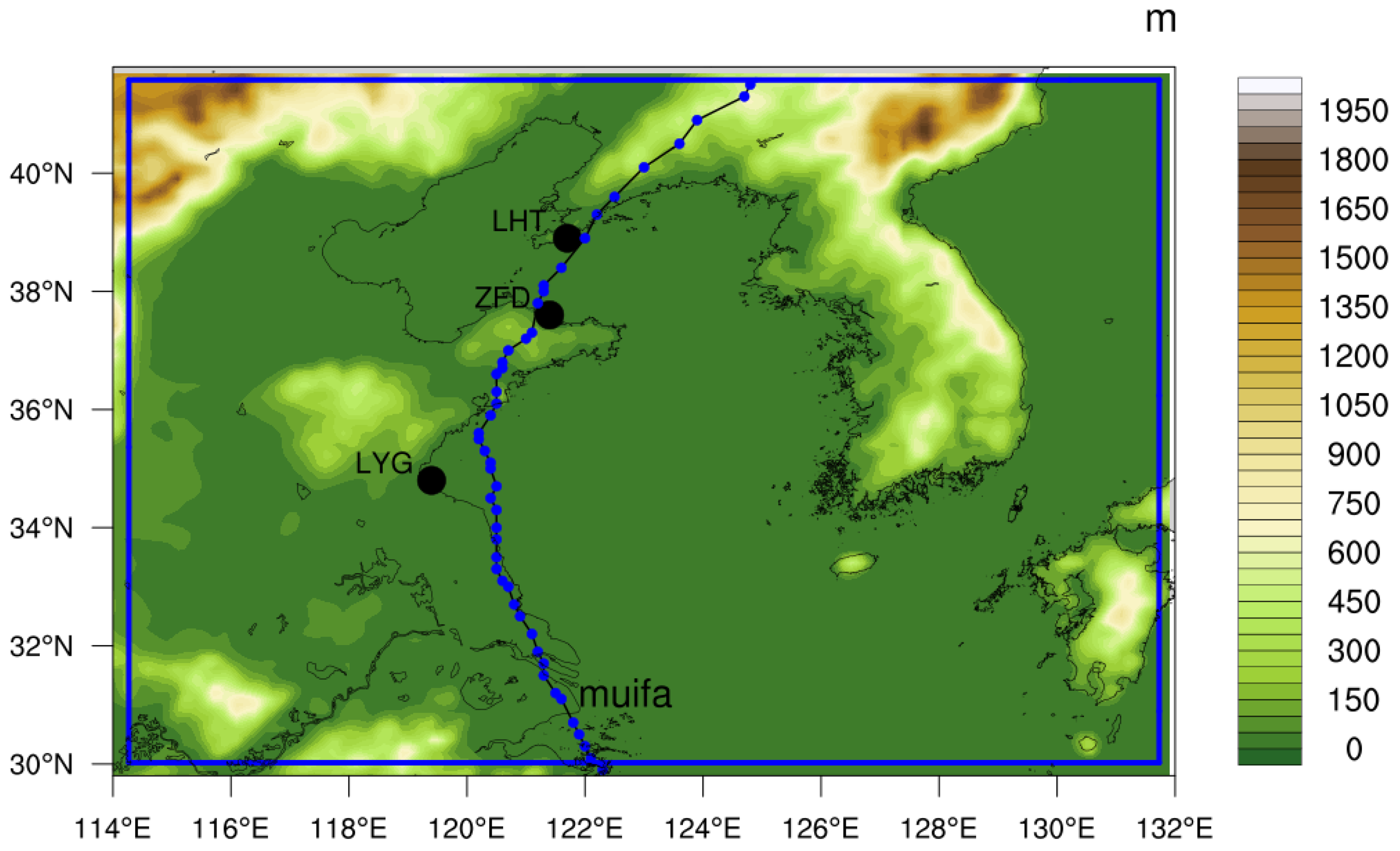
In this study, observed data of wind speed at 10 m level and significant wave height data from three buoy stations located in the Yellow Sea and Bohai Sea were utilized for correction model training and validation. The stations include Laohutan (LHT), Zhifudao (ZFD), and Lianyungang (LYG), as marked by the black dots in Figure 3. The buoy data were derived from the National Marine Science Data Center (https://mds.nmdis.org.cn/ (accessed on 3 February 2024)), with its observational frequency of once per hour.
The ECMWF Reanalysis v5 (ERA5, available online at https://cds.climate.copernicus.eu/ (accessed on 03 February 2024)) dataset is the fifth generation of atmospheric reanalysis data produced by the European Centre for Medium-Range Weather Forecasts (ECMWF). ERA5 combines general circulation models with numerous ground-based and satellite observations, resulting in ERA5 data with a spatial resolution of 0.25° × 0.25° [30,31]. He et al. evaluated the differences between ERA5 and the previous generation atmospheric reanalysis dataset (ERA-Interim) based on 30 years of observations on Chinese ground stations [32]. They found that ERA5 data were closer to the station observations, with a mean bias decrease of over 35% for surface downward shortwave radiation compared to ERA-interim.
The ERA5 data are regarded as some of the most accurate reanalysis data currently, and many studies on weather/climate mechanisms treat them as observations. Therefore, the ERA5 data were chosen for subsequent comparisons of model accuracy, in order to provide a more intuitive impression on the accuracy level of the newly established forecasting model.

3. Experimental Design

3.1. Model Configuration

In this study, the study domain (Figure 3) covered the Yellow Sea, Bohai Sea, and their surrounding areas in a shallow water depth or low-altitude terrain. The configurations of the sub-models in COAWST are as follows. The grid number of WRF was 330 × 270, with a horizontal resolution of 6 km and 39 vertical layers. The grid number of ROMS and SWAN was 320 × 260, with the same horizontal resolution as that of WRF. The 16 layers were divided in the vertical direction for the ROMS sub-model. The WRF utilized the WSM6 cloud microphysics parameterization [33], the YSU boundary layer [34], the MM5 surface layer [35], the RRTM longwave radiation [36], the Dudhia short-wave radiation [37], the Noah-LSM land surface process [38], and the GF cumulus convection scheme [39]. For the ROMS setup, turbulent mixing in the vertical direction was computed using the Mellor–Yamada scheme [40] and anisotropic currents were computed using the Flather boundary condition approach to allow free propagation of wind-generated currents and tides [41].

3.2. Optimization Process Steps for Bias Correction Models

Although the four bias correction algorithms used in this study are mature algorithms, there is significant variation in the performance of correction models constructed using different strategies in practical applications. Numerous studies demonstrated that these data-driven empirical models relied heavily on the training strategy of the model and the choice of variables used to construct the network structure. For example, Kavzoglu found that different model training strategies directly affect the accuracy of the model by 4.4~27% [42].
Therefore, prior to establishing the forecasting model, this study conducted two groups of sensitivity tests in order to obtain more accurate training dataset and variable selection scheme. The first group of sensitivity tests aimed to obtain more accurate training dataset. They investigated the influence of different simulation methods on the accuracy of the long-term dataset. The second group of sensitivity tests aimed to obtain more precise selection scheme of training variables by examining the impact of different training variable selections on the model accuracy.
The specific steps of optimization process are listed as follows.
(a)
Before creating the training data of bias correction, it is known that the errors of numerical weather models are easy to accumulate in a long-term simulation [43]. Thus, to improve the accuracy of the historical training data, we utilized the COAWST model to construct three groups of sensitivity tests (S1, S2, S3) with different time durations for a single uninterrupted simulation. The simulation in the S1 test lasted for 5 days, and the model was then restarted for the next five-day simulation. The simulation in the S2 test lasted for 15 days at each time, and the simulation in the S3 test lasted for 30 days. The simulation period for the three tests was one month. The difference in bias value was determined to confirm the impacts of simulation durations on accuracy.
(b)
According to the sensitivity test outcomes, simulation during the entire year of 2021 using COAWST was conducted over the study domain, in an operation way with the lowest bias. Considering the operation convenience and error accumulation, the simulation at each time lasted for 6 days. The simulation on the first day was used as a spin-up, and the simulation in the next five days was used to create the formal hourly training data for the establishment of bias correction models.
(c)
Before the formal training processes for the correction models, this study also constructed five sensitivity tests to investigate the impacts of different training samples on the correction accuracy. Considering the BPNN as a bias correction algorithm, the five tests (T1, T2, T3, T4, T5) used different historical simulation variables from step (b) above and observational data from three buoy stations to train the BPNN correction model. To select appropriate configurations for training variables, the accuracy difference among the five tests was analyzed. The T1 test utilized the simulations of wind speed and wave height to establish the bias correction model. The T2 test analyzed the time correlations between simulated variables at the surface and buoy observation data. All the simulated variables with a correlation coefficient of not less than 0.15 were then selected to establish a multivariate correction model. The training process in the T3 test was similar to the T2 test, but the T3 test utilized the higher correlation variables (not less than 0.4) to establish the correction model. Using the same training strategy as the T2 test, the T4 test further added the observations of the previous day from the same buoy station into the model training process. Although the T5 test followed the T1 test strategy, it also added the observations of the previous day. The T0 test was denoted as the control test without any corrections. By evaluating the accuracy of the corrected forecasts during the validation period, the training strategy with the highest accuracy could be selected for the subsequent formal training of correction models.
(d)
Based on the above test results, the formal training process of bias correction models was carried out using the hourly simulations during the entire year of 2021 and observations from three buoy stations as input data.
After the optimization process, four bias correction models were trained and established using the MOS, BPNN, LSTM, and CNN algorithms. And then, the four groups of corrected forecasts were averaged using the ensemble mean method in Section 2, and the final forecasting product was made.

3.3. Validation Test Design

For the result validation, one group of hind-cast simulations using COAWST was conducted for the entire month of September 2022. During the validation period, the hind-casts were conducted every day for the simulation of the next 72 h. By evaluating the bias compared with observations, we attempted to investigate the performance of ensemble forecasting product in correcting the forecasted bias of sea surface wind speed and wave height of COAWST. For comparison, the four groups of corrected forecasts before ensemble mean process were also presented. In addition, in order to evaluate the accuracy maintenance capabilities of the forecasts with the forecast time, the corrected forecasts of 24 h were compared with the forecasts of 48 and 72 h.

4. Result

4.1. Sensitivity Analysis Prior to the Formal Correction Model Training

4.1.1. Sensitivity of Bias on the Simulation Time Durations

According to step (a) in Section 3.2, three sensitivity tests were conducted with different time durations in a single simulation. The mean bias for the three tests at buoy stations is presented in Table 1. The mean bias of wind speed increased with the increase in simulation time. When compared to the S1 test which lasted for 5 days in each simulation, the wind speed and wave height bias increased by approximately 57% at the three stations in the S3 test which ran continuously in the 30-day simulation.
Based on the above results, the following formal simulation test could last for six days every time. The simulations on the first day were neglected as a spin-up, while the simulations on the remaining five days were collected to create the whole simulation series of one year as the training data.

4.1.2. Sensitivity of Corrected Bias on the Number of Sample Variables for Training

According to step (b) in Section 3.2, the BPNN algorithm was used to establish the sensitivity tests on the number of sample variables for training. Table 2 lists the correlation coefficients between the simulated surface variables and the observed wind speed as well as wave height during the training period. The simulated surface variables for the correlation calculation include the air temperature at 2 m level (T2M), sea surface temperature (SST), sea level pressure (SLP), relative humidity at 2 m level (RH2M), upward surface heat flux (HFX), latent heat flux (LH), upward longwave radiation (OLR), wavelength (LWAVEP), wave period (PWAVE), friction velocity in similarity theory (UST), surface pressure (PSFC), net shortwave flux at surface (GSW), wind speed at 10 m level (composed of U10 and V10 wind component at 10 m level), and significant wave height (HWAVE). Among the variables, the simulated wind speed and significant wave height had the highest correlation coefficients with the observed wind speed and wave height. According to the correlation coefficients (Table 2), the variables selected for wind training in the T2 and T4 test included T2M, SST, RH2M, HFX, LH, UST, wind speed, and HWAVE. The variables selected for wave training in the T2 and T4 test included T2M, SST, SLP, LWAVEP, PWAVE, UST, PSFC, wind speed, and HWAVE. The variables selected for the T3 test with correlation coefficients of not less than 0.4 included UST, wind speed, and HWAVE.
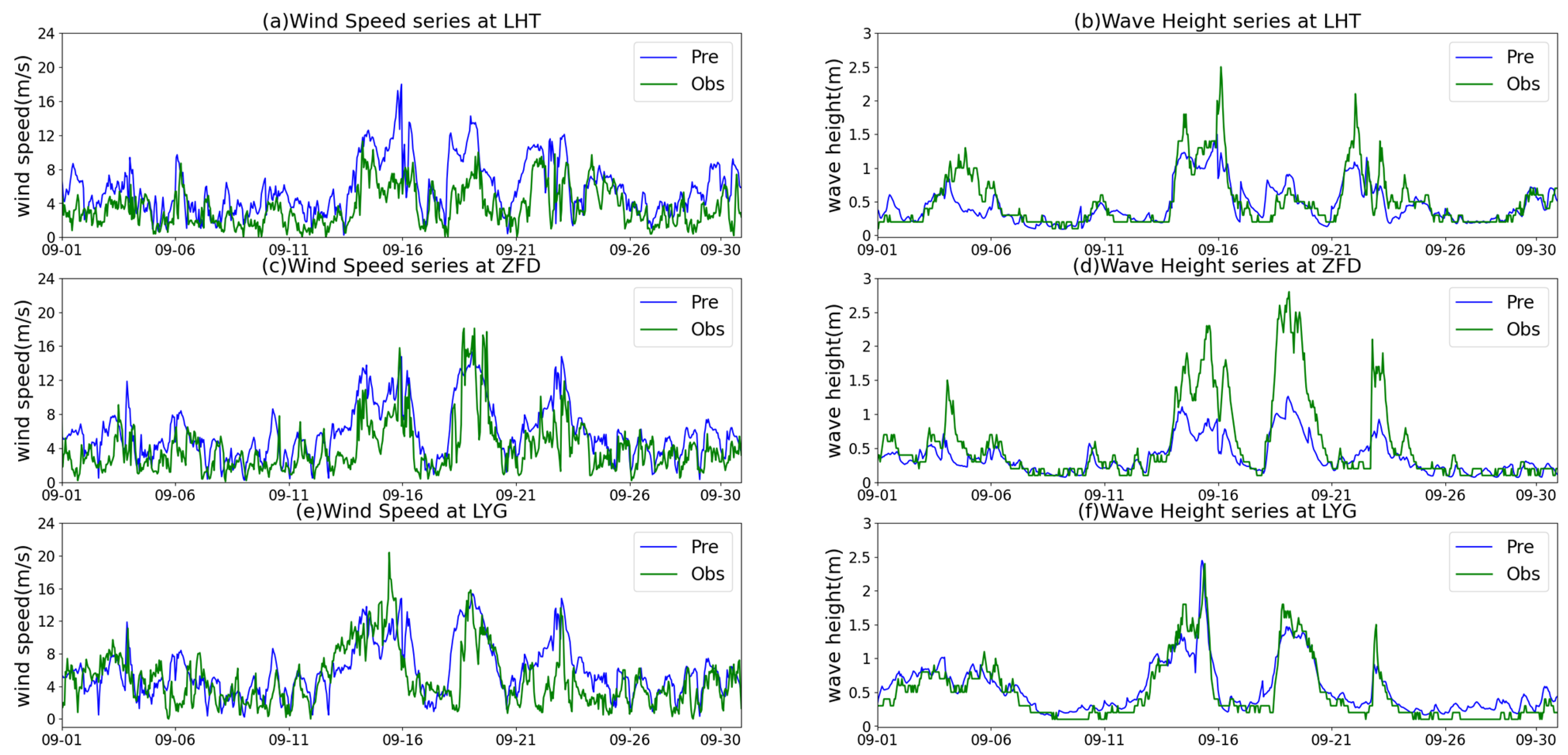
Figure 4 presents the time series of buoy observations and COAWST forecasts during the validation period. During the typhoon passage on the 15th–16th, wind speed and wave height at all three stations significantly increased. Due to subsequent weather activity, wind and waves also increased twice around the 19th and 23rd. Taking the typhoon period on the 15th–16th as an example, compared with the 13th–14th, the wind speed during the typhoon period increased by 14%, 33%, and 73%, respectively, while the wave height increased by 73%, 68%, and 139%, respectively. By comparing the forecasts and observations on the 15th–16th, the forecasting bias of COAWST increased with the growth of wind and waves. Furthermore, due to deviations between the simulated typhoon trajectory and actual conditions, the maximum forecasted wind and waves occurred at times slightly inconsistent with the observations. In terms of the overall performance during the validation period, the COAWST model was able to simulate the rapid changes in wind and waves over time under extreme weather conditions, but the magnitude of change was slightly weaker in most cases compared to the observations.
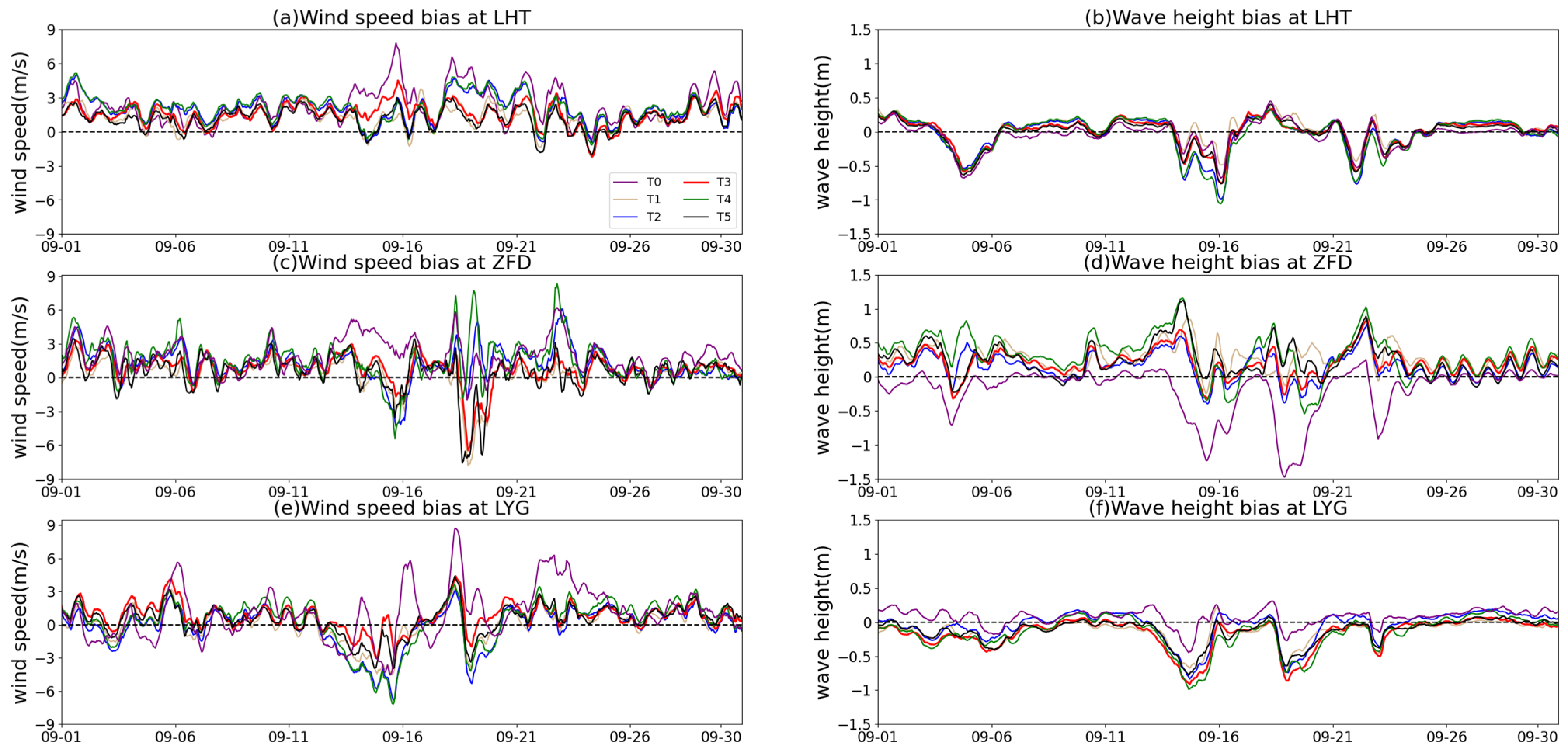
Figure 5 shows the time series of bias for the five sensitivity tests at three buoy stations during the validation period. All the series were filtered using a moving average of 12 h. Considering the wind speed bias series in Figure 5a,c,e, the lowest mean bias was detected in the T5 test with the second lowest in T1 and T3 tests. The mean bias of wind speed in the T1 test, which used a single-variable training strategy, was 1.26 m/s, 0.38 m/s, and 0.10 m/s at the three buoy stations, respectively. The bias in the T3 test, which used four variables with correlation coefficients of at least 0.4 for training, was 1.53 m/s, 0.73 m/s, and 0.78 m/s. It was slightly higher than that in the T1 test. The T2 and T4 tests, which utilized multiple variables with correlation coefficients not less than 0.15 for training, showed higher bias. The mean bias was 2 m/s, 1.22 m/s, and 0.12 m/s for the T2 test, and 1.18 m/s, 0.6 m/s, and 1.59 m/s for the T4 test, respectively. The bias in the T5 test, which added the wind speed observations in the previous day based on the training strategy of the T1 test, was 0.31 m/s, 0.06 m/s, and 0.07 m/s. It was the lowest for all the tests. Compared to the uncorrected bias in the T0 test, it reduced by 35%, 32%, and 20%. The bias series was balanced and stable without abrupt changes. For the T1 and T3 tests with the second lowest bias, the series of T3 biases were relatively more stable, and its mean bias was reduced by 28%, 29%, and 21% compared to the T0 test.
For the bias series of wave height in Figure 5b,d,f, the mean bias in the T3 test was the lowest (−0.004 m, 0.20 m, and −0.17 m) at the buoy stations. Compared to the uncorrected bias in the T0 test, the bias in the T3 test was reduced by 89%, −7%, and −143%.
Considering the performance levels of corrected wind speed and wave height, the T3 test performed best among the sensitivity tests. Table 3 lists the RMSEs of the corrected winds and waves from the five tests. The differences in RMSE among the five tests were generally consistent with the performance shown in Figure 5.
Based on the above results, the training strategy of the T3 test was used to train other correction models in the following works. It utilized the simulated variables with correlation coefficients of not less than 0.4. Although more training variables could construct more complex models, the complex models did not necessarily perform better in real operations. The way of adding variables in low correlations with target variables might induce the opposite effects. The data from the previous day played a limited role in reducing the overall bias in this training process. However, the bias even increased in some cases. Owing to the uncertainty, historical data could not be introduced for the following training processes in this study. We will conduct more tests on joint training using data from different time periods in the future.

4.2. Bias Evaluation of the Four Correction Models Using Different Algorithms

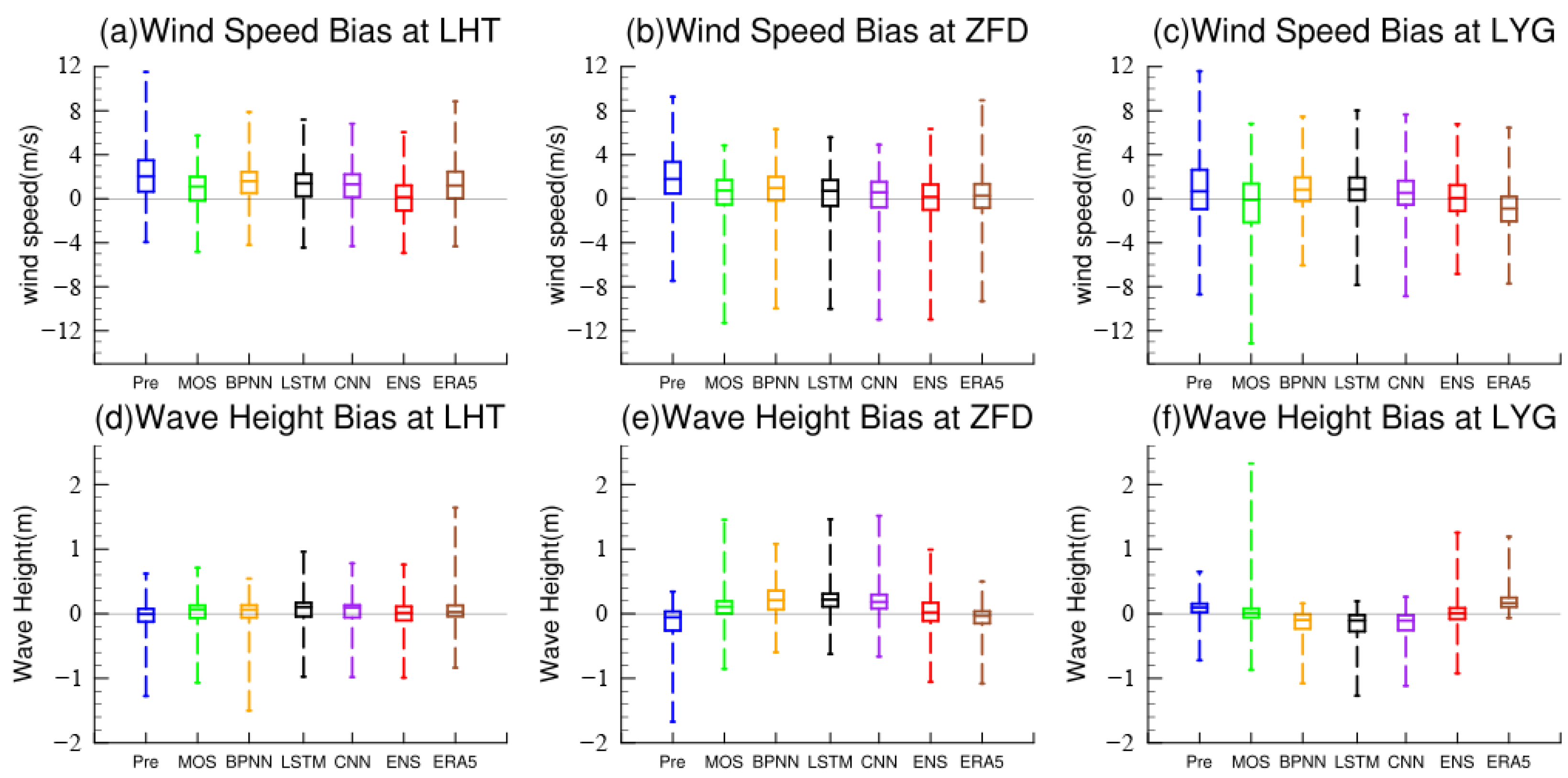
Based on the above training strategy, all of the bias correction models were established and the ensemble mean forecasts were made. Figure 6 shows the box plots of bias distribution from the ensemble mean forecasts (ENS) of wind speed and wave height, accompanied with the four groups of corrected forecasts prior to ensemble mean process. The upper and lower boundaries of the box represent the maximum and minimum values of the bias, while the middle line of the box represents the median value, reflecting the error levels of samples on average. The uncorrected forecasting bias (colored in blue) and the differences between the ERA5 reanalysis data and buoy observations (colored in brown) are also presented in Figure 6.
As shown in Figure 6a–c, the positive bias of wind speed from the COAWST’s forecasts was detected at all three buoy stations. The median values of bias were 2.03 m/s, 1.79 m/s, and 0.67 m/s, respectively. Compared to the original uncorrected forecasts, the median bias was reduced after correction and ensemble averaging. The median values of bias from the final ensemble forecasts (denoted as ENS and colored in red) were 0.14 m/s, 0.17 m/s, and 0.07 m/s, respectively. Also, the boxes between the upper and lower quartiles were shifted downwards. In most cases, the bias distributions of final ensemble forecasts became the most concentrated, and the height of the boxes was also reduced. The overall shapes of the plots did not change significantly, indicating that the final ensemble forecasts did not change the statistical distribution during bias correction and ensemble averaging.
Considering the difference among the four correction algorithms, the correction strategy of MOS was found to be more direct and aggressive, leading to a significant difference in the uncorrected forecasts of bias distribution. This strategy resulted in a bias increase at some stations. In contrast, the strategies of the other three correction models tended to be more conservative. The median bias values of wind speed corrected by CNN were 1.31 m/s, 0.57 m/s, and 0.52 m/s at the three stations, which were closest to zero among the four algorithms. For the ERA5 data as the reference, the median values were 1.19 m/s, 0.27 m/s and -0.89 m/s. It maintained a high level of data accuracy on sea surface winds.
Considering the distributions of wave height bias in Figure 6d–f, the median values of uncorrected forecasts were found to be −0.005 m, −0.05 m and 0.09 m, respectively. The correction performance for wave height was not as obvious as that for wind speed. The median bias of final ensemble forecasts was lower than any other corrected forecasting bias, with the medians of 0.011 m, 0.018 m, and 0.007 m, respectively. A special case occurred in Figure 6f. More positive bias in greater values was detected from the MOS corrections, indicating that this relatively simple algorithm is less effective in maintaining correction stability compared to others. The remaining three algorithms presented similar negative bias universally. The final ensemble forecasts combined the advantages of four bias correction algorithms through ensemble averaging, providing a more reasonable bias distribution. The wave height difference between ERA5 and observations was generally farther from the reference line 0 than the final ensemble forecasts (ENS). At certain stations, some extremely large differences between ERA5 and observations were present (Figure 6d).
Considering the bias distributions for wind speed and wave height, the final ensemble forecast demonstrated a more stable performance at different stations and was closer to the observations in terms of distributions and median values of bias.
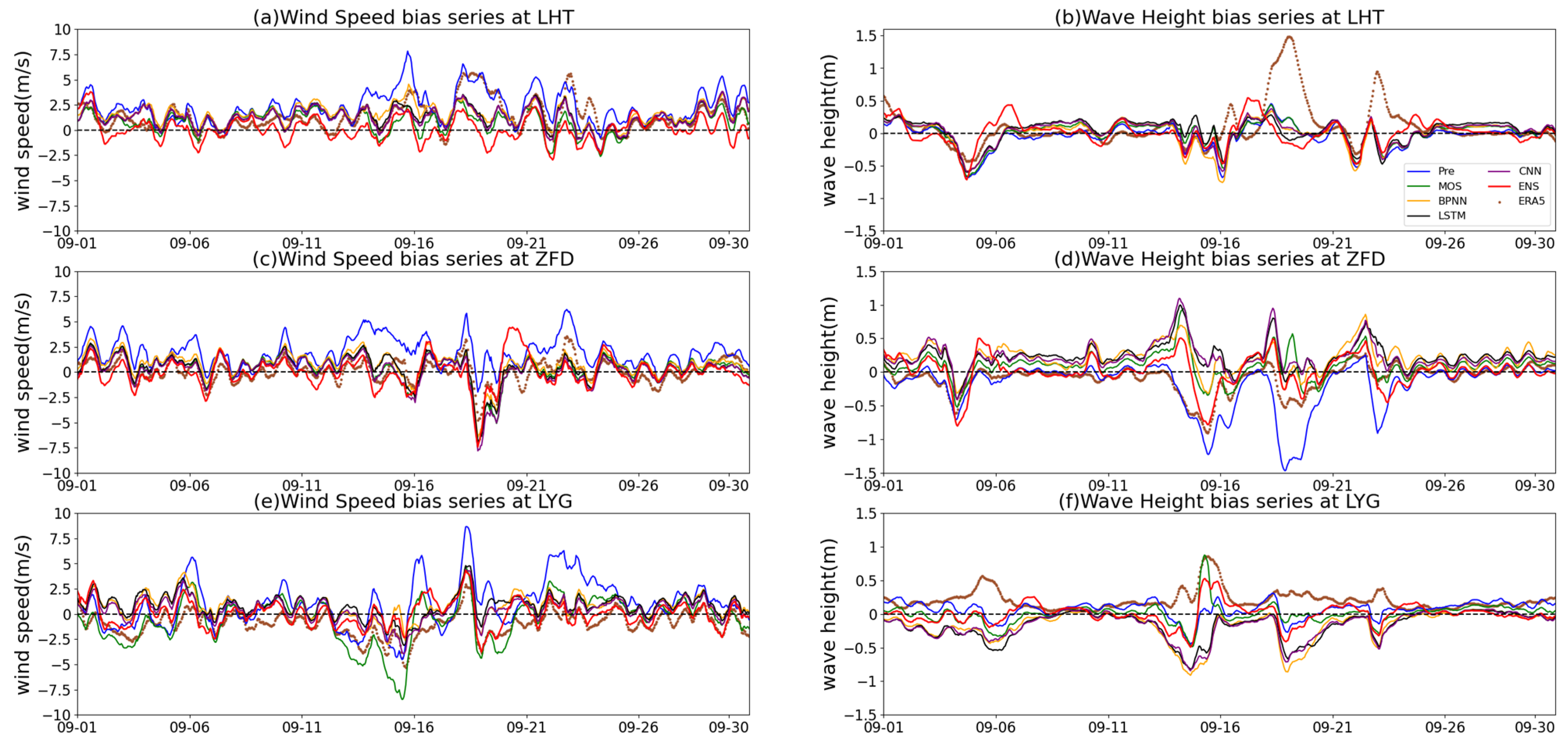
Figure 7 shows the bias series of 24 h forecasts in the validation period. All of the series were filtered using the moving average of 12 h, and the differences between ERA5 data and observations were also provided as references. As shown in Figure 6a,c,e, the uncorrected forecasts of wind speed remained a highly positive bias during the validation period, with a mean bias of 2.25 m/s, 1.89 m/s, and 0.99 m/s at the three buoy stations, respectively. After correction and ensemble averaging, the bias of final ensemble forecasts decreased to 0.09 m/s, -0.02 m/s, and 0.025 m/s. Compared to the uncorrected forecasts, the mean absolute bias was reduced by 96%, 99%, and 97%. The differences between ERA5 data and observations, with the mean values of 1.36 m/s, 0.12 m/s and −0.93 m/s, were found to be slightly lower than the uncorrected forecasting bias but still higher than the bias of final ensemble forecasts. For the four correction algorithms, the mean bias of wind speed corrected by CNN was the lowest while having the values of 1.24 m/s, 0.16 m/s, and 0.45 m/s. On 15–16 September 2022, all of the three buoy stations were affected by the Typhoon “Muifa” (Figure 3). Although the bias within the two days did not reach the peak values in the validation period, it was still maintained at a high level. The mean values of uncorrected forecasting bias were found to be 4.09 m/s, 2.95 m/s, and 3.87 m/s. By way of comparison, the mean absolute bias of wind speed ensemble forecasts was reduced by 92%, 98%, and 91%, which proved the effectiveness of ensemble forecasts in extreme weather conditions.
As shown in Figure 7b,d,f, the mean bias values of uncorrected wave height were −0.04 m, −0.19 m, and 0.07 m, respectively. The bias reduction effects on wave height from the final ensemble forecasts were not as significant as those on wind speed. The wave height series of ERA5 data, however, also showed a high uncertainty in data accuracy. A large positive difference at the Laohutan station (Figure 7b) was detected, which was obviously greater than any forecast series. For the four bias correction algorithms, the lowest mean bias was detected from the series corrected by the simplest MOS algorithm, with values of 0.005 m, 0.09 m, and 0.002 m at the three buoy stations. When the typhoon passed the buoy stations on 15–16 September, the MOS correction model reduced the mean absolute bias of wave height by 34%, 75%, and 86%. After the typhoon, the wave height forecasts still maintained a high bias level for several days due to the residual weather processes. At Lianyungang station in Figure 7f, the other three correction forecasts, except for the MOS corrections, showed significant negative bias, which might be induced by the overfittings of the neural networks. The three correction algorithms based on the neural network building in different complexity (BPNN, CNN, and LSTM) did not capture the entire characteristics of waves at the Lianyungang station, and provided optimal estimations with deviations in the correction processes. Relying on dynamically changing weights, the final ensemble forecasts achieved the mean bias of 0.003 m, 0.011 m, and −0.001 m even when significant bias was present in three of the correction algorithms. During the typhoon passage period (15–16 September), some correction algorithms even exhibited larger bias than the uncorrected forecasts, while the simplest MOS method performed well during this period, successfully reducing the mean bias of wave height by 34%, 75%, and 86%. Although other algorithms had a relatively larger bias, the weight of MOS did not reach 100% in the ensemble mean process. Thus, the ensemble mean results did not yield a lower bias than the MOS algorithm on the 15th–16th, with the mean bias reduced by 56%, 43%, and 16%.
In extreme weather, the bias of numerical forecasts was believed to increase accordingly, and the COAWST model was no exception. For the ensemble forecasts in this study, in addition to the increased bias, the extreme weather also posed new challenges. First, due to the drastic weather changes, it was unknown whether the bias statistics in the previous day was representative of the current model bias. Second, it was unclear whether the four correction algorithms could react in time by recognizing the rapidly increased bias at this stage. In terms of practical performance, the final ensemble forecasts were able to adapt to these challenges in extreme weather, and the performance was generally better than in normal weather.
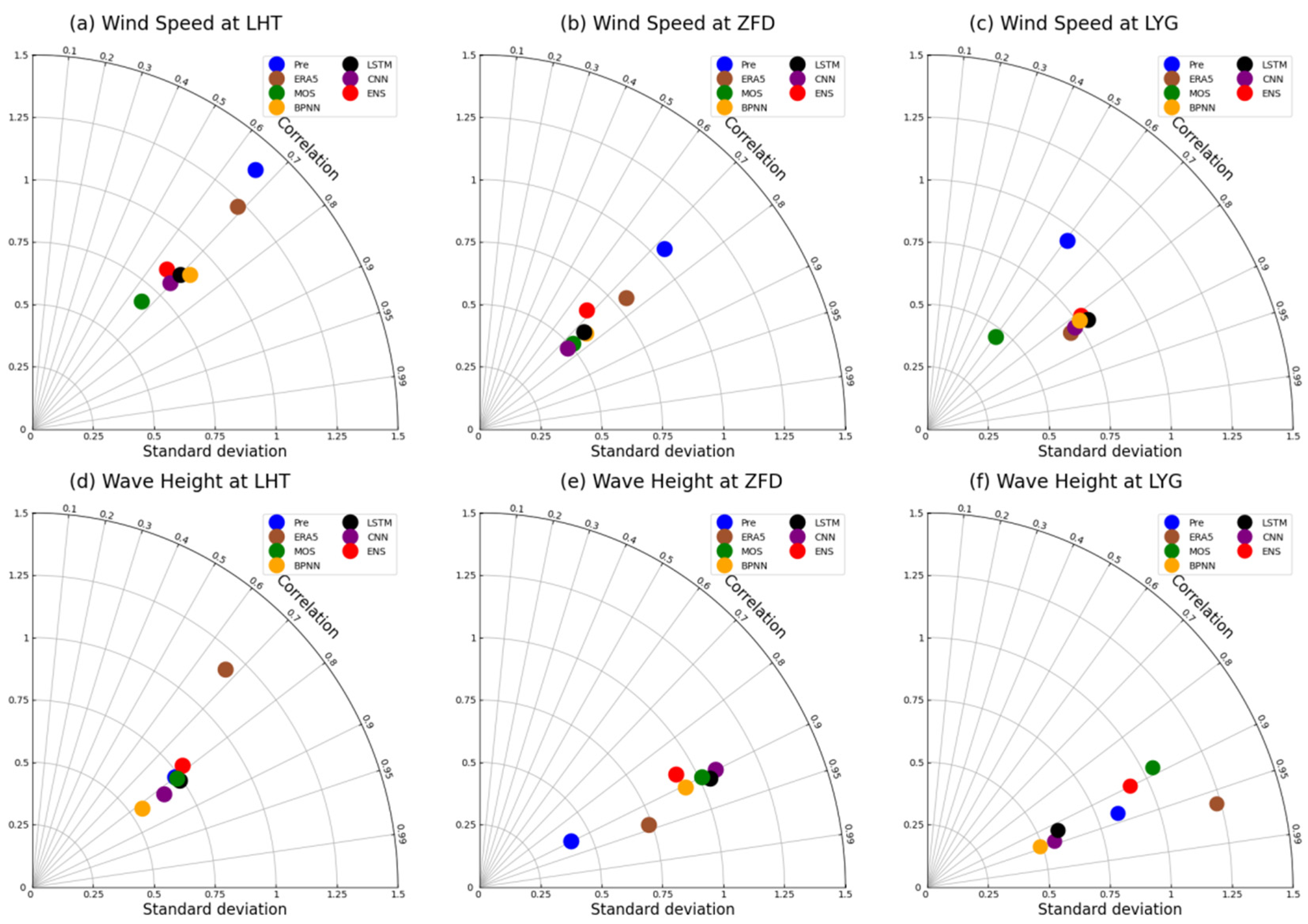
Figure 8 shows the Taylor diagram of the forecasting results during the validation period. The Taylor diagram includes a standard deviation dimension and a correlation coefficient dimension. If one series stays closer to the reference dot (the crossing dot of the arc line 1 and x-axis), the statistical indices of the series remain higher.
As shown in Figure 8a–c, the indices of corrected wind speed were improved by different degrees. The most significant improvements were detected at Lianyungang station. However, the standard deviations of ensemble and correction results were generally lower than those of the observations and uncorrected forecasts, which was consistent with the distributions of extreme bias in Figure 6a–c. This indicated that the correction models reduced the oscillation amplitudes of the forecasting series by different degrees. For the correlation coefficient, there were no significant differences between these corrected series and the uncorrected ones. The performance of the MOS correction model with the simplest algorithm was not as stable as the others and presented lower deviations of wind speed in Figure 8a,c.
As shown in Figure 8d–f, the corrected series generally remained consistent with the observations for correlation coefficient but differed for standard deviation. Despite of the performance uncertainties among the three stations, the final ensemble forecasts always appeared at locations nearer to the reference dot. The final ensemble forecasts had a slightly reduced correlation coefficient compared to other correction results, but this drawback was compensated for by the improvement in standard deviation. In other words, the final ensemble forecasts might not provide the best performance in specific cases or statistical indices, but it always minimized uncertainties across all cases.

4.3. Accuracy Changes in the Ensemble Mean Forecasts with Different Forecasting Time

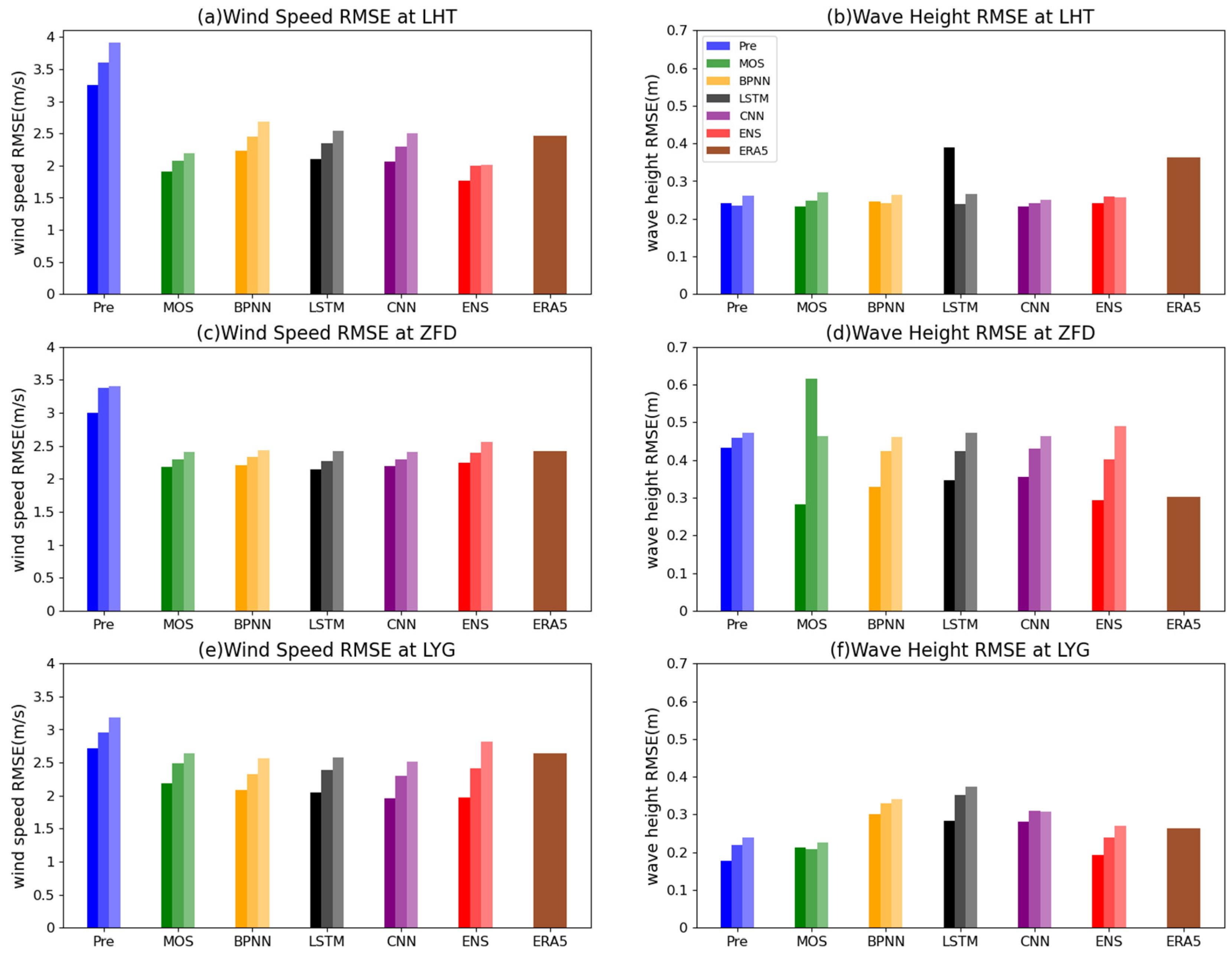
To investigate whether the ensemble forecasts were able to maintain the accuracy with different forecasting times, Figure 9 shows the bar charts of RMSE for the forecasts of 24, 48, and 72 h ahead. As shown in Figure 9a,c,e, the RMSE of wind speed increased with the increase in the forecasting time. Among them, the uncorrected forecasts had the highest errors while having the RMSE values of 3.25 m/s, 2.99 m/s, and 2.99 m/s for the 24 h forecasts at the three buoy stations. The RMSEs of the corrected forecasts were significantly lower than those of uncorrected ones, which was identical to the mean bias performance. With the increase in forecast time, the bias increased by 4~30% and the errors were almost equally spaced. This indicated that within the forecasting period of 72 h, the correction accuracy for wind speed could be maintained without any failure or distortion. By assigning greater weights to the correction models with lower bias, the RMSEs of the final ensemble forecasts were further reduced. The RMSEs of the 24 h ensemble forecast were 1.76 m/s, 2.24 m/s, and 1.97 m/s, respectively. As the forecasting time increased, the RMSE growth rate of the ensemble forecasts was slightly faster than that of the individual correction models, which also meant that it was difficult to maintain a high accuracy by using observation data from the previous 48 or 72 h to estimate model weights at the current time.
In addition, the RMSEs of ERA5 data at the three stations were 2.45 m/s, 2.41 m/s, and 2.64 m/s, respectively. When compared to the ensemble forecasts, the ERA5 data did not show a superiority in accuracy.
Figure 9b,d,f show the RMSEs of wave height. Unlike the stable increase in wind speed errors, higher variability was detected in the errors of corrected wave height. The RMSEs of uncorrected forecasts were 0.24 m, 0.43 m, and 0.17 m, respectively. This error level was not the highest among all the results; instead, it was even lower than the error level of ERA5 data at Laohutan and Lianyungang stations. For the four correction algorithms, the bias was reduced in most cases, but the reduction was less significant compared to the wind speed corrections. With the increase in the forecasting time, the wave height corrections also showed an increasing trend of errors. However, it had a few exceptions. For instance, the corrected forecasts of 48 h ahead by LSTM had lower errors compared to the forecasts of 24 h ahead at Laohutan station. The MOS correction model presented the lowest RMSEs while having values of 0.23 m, 0.28 m, and 0.21 m for the corrected forecasts of 24 h ahead at the three stations. By assigning more weights to the MOS correction results, the RMSEs of final ensemble forecasts for wave height were 0.24 m, 0.29 m, and 0.19 m. Such results indicated that for more challenging wave height forecasts, ensemble forecasts effectively maintained forecast accuracy even when there was significant uncertainty in the correction algorithm’s effectiveness. Additionally, the ERA5 data did not demonstrate higher accuracy than the ensemble forecasts, with the RMSEs of 0.36 m, 0.30 m, and 0.26 m.
Table 4 shows the differences in temporal correlation coefficient between the corrected forecasts and the uncorrected ones. Compared to the corrected wind speed forecasts of 24 h ahead, there were no significant changes in the correlation coefficients for the corrected forecasts of 48 and 72 h ahead. The BPNN algorithm provided the largest promotion in correlation coefficients, followed by CNN and LSTM. The MOS algorithm provided the lowest mean bias of wave height but reduced the correlation coefficients of wave height at nearly all the stations. For the final ensemble forecasts, the correlation coefficients of wind speed and wave height slightly decreased in most cases. The result was consistent with the findings in Figure 8. The ensemble approach employed in this study focused on reducing the mean bias, which might alter the temporal coherence of the original forecasts. However, this alteration was not significant, as the changes in correlation coefficients did not exceed 0.1.

5. Discussion

Even though this study conducted research on improving the forecasts of winds and waves, there are still some limitations and uncertainties that need to be addressed in future work.
First, the data only from three buoys were selected in this study due to the limited availability of long-term public buoy data over the domain, which added more randomness to the results and conclusions. The model established in this study exhibited higher in situ forecast accuracy at several buoy locations compared to ERA5 data; however, the randomness from individual stations may pose great challenges in improving the regional forecasting accuracy when applied to specific areas.
Due to the uncertainty of buoy data from different stations, no correction algorithms could guarantee effective bias correction for all stations. As mentioned above, when correcting wave height forecasts at the Lianyungang station, the BPNN, CNN, and LSTM algorithms collectively exhibited a significant negative bias. In this case, the MOS algorithm with a smaller bias maintained the final ensemble forecasts within a low level of bias through providing larger weights. However, if all four correction algorithms exhibit a large bias at a particular location, the ensemble mean method in this study will become less ineffective. To reduce the probability of this situation occurring, it is necessary to select more algorithms based on different principles to be included in the ensemble members to address this risk.
Additionally, the hydro-meteorological conditions are complex in the land–sea border areas, and the strong localized characteristics of winds and waves are difficult to simulate. The three buoy stations in this study are located in the offshore area, which is significantly influenced by local environments. This may also affect the correction performance. We would construct the simulations in a higher resolution and optimized scheme configurations to obtain more accurate training data and correction performance at a regional level in the future.
Second, the training data were from the forecasts and buoy data lasting for only one year. In order to fit the hourly simulations of COAWST, the buoy data were averaged in each hour. Therefore, there were only 365 × 24 groups of training samples. The bias correction models in this study are essentially empirical models established based on data mining. Further expanding the training sample may be one of the effective ways to improve the correction accuracy. CNN and LSTM, two deep learning algorithms, may be most affected by the sample size. Deep learning algorithms rely on large amounts of data to create more accurate data mappings. However, the advantages of deep learning algorithms were not fully presented in this study due to the limitation in sample size. In the future, it is necessary to conduct simulations for longer time durations and higher resolutions to increase the sample size of the training data. It is ideal for the data exploration of more accurate nonlinear relationships between forecasts and observations. If, with more training data, the potential improvement in the effectiveness of these two deep learning algorithms (CNN and LSTM) remains unknown, then their stability is probably to be enhanced.
Additionally, this study did not extract additional features from the training data. Some previous studies showed that feature extraction methods, such as the ensemble empirical mode decomposition (EEMD) and principal component analysis (PCA), were also effective in increasing sample sizes and good for accuracy promotion [44]. Also, it is another way to increase the sample size by incorporating forecast data from neighboring grids into the model training. However, caution must be exercised when employing this approach because the local characteristics of wind and waves are highly pronounced, and grid points that are too far away may not be representative. In summary, we will also conduct detailed research on the processing methods for training data in the future.
Third, this study utilized only four popular algorithms for bias correction. Based on the results of this study, the ensemble scheme needs to introduce more algorithms with different principles to enhance environmental adaptability and avoid the phenomenon of collective bias among all neural network algorithms at the Lianyungang station. Therefore, machine learning algorithms such as support vector machine (SVM), extreme gradient boosting (XGBoost), random forest (RF), etc., are preferred targets. Algorithms with significant differences in neural network structures from CNN and LSTM can also be considered, such as Generative Adversarial Networks (GAN) or Multi-Layer Perceptron (MLP).
Despite the inherent uncertainties in results, the developed ensemble forecasting system in this study has demonstrated high potential for application. In practical use, the main limiting factor of this system stems from having sufficient observation data rather than regional hydro-meteorological differences. In new application locations, bias correction algorithms require an ample amount of training data to establish a new empirical local relationship, as such local empirical relationships are challenging to directly transfer to other locations. For regional forecasting, many studies on regional bias correction are based on two-dimensional data, typically reanalysis data, for training. This allows for the improvement of regional statistical indices through the trained “forecast-observation” mapping relationship. However, when it comes to specific individual stations, their forecasting accuracy may not surpass the in situ correction effect utilized in this study. After all, even the reanalysis data used as the training benchmark cannot guarantee low errors at all stations.

6. Conclusions

The forecasts of winds and waves at the sea surface are closely related to human activities. However, a large bias is still present in operational forecasts. Artificial intelligence-based bias correction methods have been used more often in recent years and the correction results have also proved to be efficient. Therefore, four bias correction algorithms—MOS, BPNN, CNN, and LSTM—were used in this study to correct the forecasts of COAWST. And then, based on these corrected forecasts, a resemble forecasting model was established for three buoy stations over the Yellow Sea and Bohai Sea using a simple bias-removed ensemble averaging scheme. The training data for the correction models were obtained from historical simulations of COAWST and observation data throughout the year 2021. During the validation period in September 2022, several sensitivity tests were conducted to obtain accurate establishment strategy of bias correction models, and formal evaluations on the final resemble forecasts were then presented. This study aimed to analyze the impacts of training strategies on the accuracy of bias corrections and evaluate the performance levels of established ensemble forecasting product. The conclusions are listed as follows.
(1)
The errors accumulated in the long-term continuous simulations using numerical weather models and the rates of error accumulation for the rapidly changing wind speed were more obvious than that for the wave height at a slower changing rate.
(2)
In the correction model training process, the accuracy of the trained models depended on the sample size of training data that was strongly correlated to the target variable. The inclusion of data having a low correlation with the target variable might decrease the accuracy of the correction model. The way of introducing observations of the previous days directly into the training process did not significantly change the accuracy of the correction model.
(3)
After bias correction by the four algorithms, the wind speed forecasts were improved in most statistical indices. However, the corrected wave height forecast did not present significant improvements. Certain uncertainties were still present for wave height corrections for different statistical indices at different stations. Due to these uncertainties, none of the four algorithms presented a stable lowest bias at all stations. Relying on the dynamic weight assignment, the final ensemble forecast greatly reduced the uncertainties from different stations. In cases where the accuracy of a certain correction algorithm significantly surpassed other algorithms, the ensemble forecast might not have the lowest bias, but its accuracy was undoubtedly the most stable among all cases. In addition, the ensemble forecasts might slightly reduce the correlation with observations, but the improvement in forecasting bias and standard deviation could compensate for this issue.
(4)
In terms of the specific performance of bias correction, the mean bias of wind speed forecasts from COAWST was found to be 2.31 m/s~2.58 m/s at three buoy stations. The 24 h ensemble forecast further reduced the mean absolute bias by approximately 96~99%. When the Typhoon “Muifa” passed across the domain, the representativeness of the model weights calculated using the previous day’s observations was decreased. Their mean absolute bias reduced by 91~98%, and surpassed the statistical indices of ERA5 reanalysis data in most cases. For wave height forecasts with higher uncertainty, the mean bias of original COAWST forecast was −0.19 m~0.07 m, while the 24 h ensemble forecast still reduced the mean by approximately 91~95% even in cases where several correction results increased the bias, and during typhoon periods, it reduced by 16~54%. Within the forecasting period of 72 h, the effectiveness of weight distribution in ensemble forecasts gradually decreased with the extension of time, and the accuracy of the 72 h ensemble forecast was not as good as the individual corrected forecast results. This indicated that for rapidly changing wind speed and wave height, the empirical rules relying on the 24 h bias performance were difficult to apply over longer time periods in this study.
(5)
Considering the differences among the four correction models, there was no direct co-relationship between the correction accuracy and the complexity of each algorithm. However, the relatively complex algorithms (CNN and LSTM) presented more conservative correction strategies at different stations, resulting in more stable performance. The MOS correction model with the simplest algorithm presented a more direct and aggressive correction strategy, which resulted in an unstable correction performance. Although the mean bias of wave height corrected by MOS was the lowest, the bias might increase significantly after correction in some cases. In this study, the correction performance of the BPNN algorithm was very similar to that of deep learning algorithms (CNN and LSTM). The BPNN performed slightly better than CNN in correcting wave height and promoting the correlation coefficients with observations.

Author Contributions

Project administration, J.Z.; writing—original draft preparation, T.Z.; software, Y.L.; validation, Z.Q.; resources, B.W.; writing—review and editing, C.C.; supervision, Z.L.; Conceptualization, T.H. and Y.G.; All authors have read and agreed to the published version of the manuscript.

Funding

This research was funded by [the Key R&D Program of Shandong Province, China] grant number [2023ZLYS01], [the National Natural Science Foundation of China] grant number [42076195, 42206188, 42176185, 42206001], and [the Natural Science Foundation of Shandong province, China] grant number [ZR2022MD100], [the “Four Projects” of computer science] grant number [2021JC02002], [the basic research foundation in Qilu University of Technology] grant number [2023PY004, 2023PY050, 2023JBZ02].

Institutional Review Board Statement

Not applicable.

Informed Consent Statement

Not applicable.

Data Availability Statement

The data presented in this study are available on request from the corresponding author. The data are not publicly available due to internal policy of Institute of Oceanographic Instrumentation, Qilu University of Technology.

Conflicts of Interest

The authors declare no conflict of interest.

References

  1. Aija, S.; Rogers, W.E.; Babanin, A.V. Wave spectral response to sudden changes in wind direction in finite-depth waters. Ocean Model. 2015, 103, 98–117. [Google Scholar] [CrossRef]
  2. Huang, F.; Garrison, J.; Leidner, S.; Grieco, G.; Annane, B. Assimilation of GNSS reflectometry delay-Doppler maps with a two-dimensional variational analysis of global ocean surface winds. QJR Meteorol. Soc. 2021, 147, 2469–2489. [Google Scholar] [CrossRef]
  3. Li, Z. Impact of assimilating Mode-S EHS winds in the Met Office’s high-resolution NWP model. Meteorol. Appl. 2021, 28, e1989. [Google Scholar] [CrossRef]
  4. Sannasiraj, S.A.; Goldstein, M.G. Optimal interpolation of buoy data into a deterministic wind–wave model. Nat. Hazards 2009, 49, 261–274. [Google Scholar] [CrossRef]
  5. Sweeney, C.P.; Lynch, P.; Nolan, P. Reducing errors of wind speed forecasts by an optimal combination of post-processing methods. Meteorol. Appl. 2013, 20, 32–40. [Google Scholar] [CrossRef]
  6. Lakatos, M.; Lerch, S.; Hemri, S.; Baran, S. Comparison of multivariate post-processing methods using global ECMWF ensemble forecasts. Q. J. R. Meteorol. Soc. 2023, 149, 856–877. [Google Scholar] [CrossRef]
  7. Cuo, L.; Pagano, T.C.; Wang, Q.J. A review of quantitative precipitation forecasts and their use in short- to medium-range streamflow forecasting. J. Hydrometeorol. 2011, 12, 713–728. [Google Scholar] [CrossRef]
  8. Li, W.; Pan, B.; Xia, J.; Duan, Q. Convolutional neural network-based statistical post-processing of ensemble precipitation forecasts. Hydrology 2022, 605, 127301. [Google Scholar] [CrossRef]
  9. Kunić, Z.; Ženko, B.; Boshkoska, B.M. FOCUSED–Short-Term Wind Speed Forecast Correction Algorithm Based on Successive NWP Forecasts for Use in Traffic Control Decision Support Systems. Sensors 2021, 21, 3405. [Google Scholar] [CrossRef]
  10. Bi, K.; Xie, L.; Zhang, H.; Chen, X.; Gu, X.; Tian, Q. Accurate medium-range global weather forecasting with 3D neural networks. Nature 2023, 619, 533–538. [Google Scholar] [CrossRef]
  11. Zhang, Y.; Long, M.; Chen, K.; Xing, L.; Jin, R.; Jordan, M.I. Skilful nowcasting of extreme precipitation with NowcastNet. Nature 2023, 619, 526–532. [Google Scholar] [CrossRef] [PubMed]
  12. Kim, H.; Ham, Y.G.; Joo, Y.S.; Son, S.W. Deep learning for bias correction of MJO prediction. Nat Commun. 2021, 12, 3087. [Google Scholar] [CrossRef] [PubMed]
  13. Wyszogrodzki, A.A.; Liu, Y.; Jacobs, N.; Childs, P.; Zhang, Y.; Roux, G.; Warner, T.T. Analysis of the surface temperature and wind forecast errors of the NCAR-AirDat operational CONUS 4-km WRF forecasting system. Meteorol. Atmos. Phys. 2013, 122, 125–143. [Google Scholar] [CrossRef]
  14. Jacondino, W.D.; Nascimento, A.L.; Calvetti, L.; Fisch, G.; Beneti, C.A.A.; Paz, S.R. Hourly day-ahead wind power forecasting at two wind farms in northeast Brazil using WRF model. Energy 2021, 230, 120841. [Google Scholar] [CrossRef]
  15. Han, L.; Chen, M.; Chen, K.; Chen, H.; Zhang, Y. A Deep Learning Method for Bias Correction of ECMWF 24–240h Forecasts. Atmos. Sci. 2021, 38, 1444–1459. [Google Scholar] [CrossRef]
  16. Chen, Y.; Bai, M.; Zhang, Y.; Liu, J.; Yu, D. Multivariable space-time correction for wind speed in numerical weather prediction (NWP) based on ConvLSTM and the prediction of probability interval. Earth Sci. Inform. 2023, 16, 1953–1974. [Google Scholar] [CrossRef]
  17. Zou, J.; Zhan, C.; Song, H.; Hu, T.; Qiu, Z.; Wang, B.; Li, Z. Development and evaluation of a hydrometeorological forecasting system using the Coupled Ocean-Atmosphere-Wave-Sediment Transport (COAWST) Model. Adv. Meteorol. 2021, 2021, 6658722. [Google Scholar] [CrossRef]
  18. Liu, N.; Ling, T.; Wang, H.; Zhang, Y.; Gao, Z. Numerical simulation of Typhoon Muifa (2011) using a Coupled Ocean-Atmosphere-Wave-Sediment Transport (COAWST) modeling system. J. Ocean Univ. 2015, 14, 199–209. [Google Scholar] [CrossRef]
  19. Ebuchi, N.; Graber, H.C.; Caruso, M.J. Evaluation of Wind Vectors Observed by QuikSCAT/SeaWinds Using Ocean Buoy Data. J. Atmos. Ocean. Technol. 2002, 19, 2049–2062. [Google Scholar] [CrossRef]
  20. Warner, J.C.; Armstrong, B.; He, R.; Zambon, J.B. Development of a Coupled Ocean–Atmosphere–Wave–Sediment Transport (COAWST) Modeling System. Ocean Model. 2010, 35, 230–244. [Google Scholar] [CrossRef]
  21. Olabarrieta, M.; Warner, J.C.; Armstrong, B.; Zambon, J.B.; He, R. Ocean–atmosphere dynamics during Hurricane Ida and Nor’Ida: An application of the coupled ocean–atmosphere–wave–sediment transport (COAWST) modeling system. Ocean Model. 2012, 43–44, 112–137. [Google Scholar] [CrossRef]
  22. Zambon, J.B.; He, R.; Warner, J.C. Investigation of hurricane Ivan using the coupled ocean–atmosphere–wave–sediment transport (COAWST) model. Ocean Dyn. 2014, 64, 1535–1554. [Google Scholar] [CrossRef]
  23. Bai, P.; Ling, Z.; Liu, C.; Wu, J.; Xie, L. Effects of tidal currents on winter wind waves in the Qiongzhou Strait: A numerical study. Acta Oceanol. 2020, 39, 33–43. [Google Scholar] [CrossRef]
  24. Lazić, L.; Pejanović, G.; Živković, M.; Ilić, L. Improved wind forecasts for wind power generation using the Eta model and MOS (Model Output Statistics) method. Energy 2014, 73, 567–574. [Google Scholar] [CrossRef]
  25. Rumelhart, D.E.; Hinton, G.E.; Williams, R.J. Learning representations by back-propagating errors. Nature 1986, 323, 533–536. [Google Scholar] [CrossRef]
  26. Li, T. Back-propagation neural network for long-term tidal predictions. Ocean Eng. 2004, 31, 225–238. [Google Scholar]
  27. Hochreiter, S.; Schmidhuber, J. Long Short-Term Memory. Neural Comput. 1997, 9, 1735–1780. [Google Scholar] [CrossRef]
  28. Zarándy, Á.; Rekeczky, C.; Szolgay, P.; Chua, L.O. Overview of CNN research: 25 years history and the current trends. In Proceedings of the IEEE International Symposium on Circuits and Systems (ISCAS), Lisbon, Portugal, 24–27 May 2015; pp. 401–404. [Google Scholar]
  29. Ince, T.; Kiranyaz, S.; Eren, L.; Askar, M.; Gabbouj, M. Real-Time Motor Fault Detection by 1-D Convolutional Neural Networks. IEEE Trans. Ind. Electron. 2016, 63, 7067–7075. [Google Scholar] [CrossRef]
  30. Napoli, C.D.; Barnard, C.; Prudhomme, C.; Cloke, H.L.; Pappenberger, F. ERA5-HEAT: A global gridded historical dataset of human thermal comfort indices from climate reanalysis. Geosci. Data J. 2021, 8, 2–10. [Google Scholar] [CrossRef]
  31. Urban, A.; Napoli, C.D.; Cloke, H.L.; Kyselý, J. Evaluation of the ERA5 reanalysis-based Universal Thermal Climate Index on mortality data in Europe. Environ. Res. 2021, 198, 111227. [Google Scholar] [CrossRef]
  32. He, Y.; Wang, K.; Feng, F. Improvement of ERA5 over ERA-Interim in Simulating Surface Incident Solar Radiation throughout China. J. Clim. 2021, 34, 3853–3867. [Google Scholar] [CrossRef]
  33. Yang, S.; Li, D.; Chen, L.; Liu, Z.; Huang, X.; Pan, X. The Regularized WSM6 Microphysical Scheme and Its Validation in WRF 4D-Var. Adv. Atmos. Sci. 2023, 40, 483–500. [Google Scholar] [CrossRef]
  34. Hong, S.; Noh, Y.; Dudhia, J. A New Vertical Diffusion Package with an Explicit Treatment of Entrainment Processes. Mon. Weather Rev. 2006, 134, 2318–2341. [Google Scholar] [CrossRef]
  35. Beljaars, C.M. The parametrization of surface fluxes in large-scale models under free convection. Q. J. R. Meteorol. Soc. 1995, 121, 255–270. [Google Scholar]
  36. Mlawer, E.J.; Taubman, S.J.; Brown, P.D.; Iacono, M.J.; Clough, S.A. Radiative transfer for inhomogeneous atmospheres: RRTM, a validated correlated-k model for the longwave. J. Geophys. Res. 1997, 102, 16663–16682. [Google Scholar] [CrossRef]
  37. Dudhia, J. Numerical Study of Convection Observed during the Winter Monsoon Experiment Using a Mesoscale Two-Dimensional Model. J. Atmos. Sci. 1989, 46, 3077–3107. [Google Scholar] [CrossRef]
  38. Chen, F.; Dudhia, J. Coupling an Advanced Land Surface–Hydrology Model with the Penn State–NCAR MM5 Modeling System, Part I: Model Implementation and Sensitivity. Mon. Weather Rev. 2001, 129, 569–585. [Google Scholar] [CrossRef]
  39. Gao, Y.; Leung, L.R.; Zhao, C.; Hagos, S. Sensitivity of U.S. summer precipitation to model resolution and convective parameterizations across gray zone resolutions. J. Geophys. Res. Atmos. 2017, 122, 2714–2733. [Google Scholar] [CrossRef]
  40. Mellor, G.L.; Yamada, T. Development of a turbulence closure model for geophysical fluid problems. Rev. Geophys. 1982, 20, 851–875. [Google Scholar] [CrossRef]
  41. Flather, R.A. A tidal model of the north-west European continental shelf. M´emoires de la Soci´et´e Royale des Sciences de Li’ege 1976, 6, 141–164. [Google Scholar]
  42. Kavzoglu, K. Increasing the accuracy of neural network classification using refined training data. Environ. Model. Softw. 2009, 24, 850–858. [Google Scholar] [CrossRef]
  43. Brunetti, M.; Vérard, C. How to reduce long-term drift in present-day and deep-time simulations? Clim Dyn. 2018, 50, 4425–4436. [Google Scholar] [CrossRef]
  44. Wu, Q.; Peng, C. Wind Power Generation Forecasting Using Least Squares Support Vector Machine Combined with Ensemble Empirical Mode Decomposition, Principal Component Analysis and a Bat Algorithm. Energies 2016, 9, 261. [Google Scholar] [CrossRef]
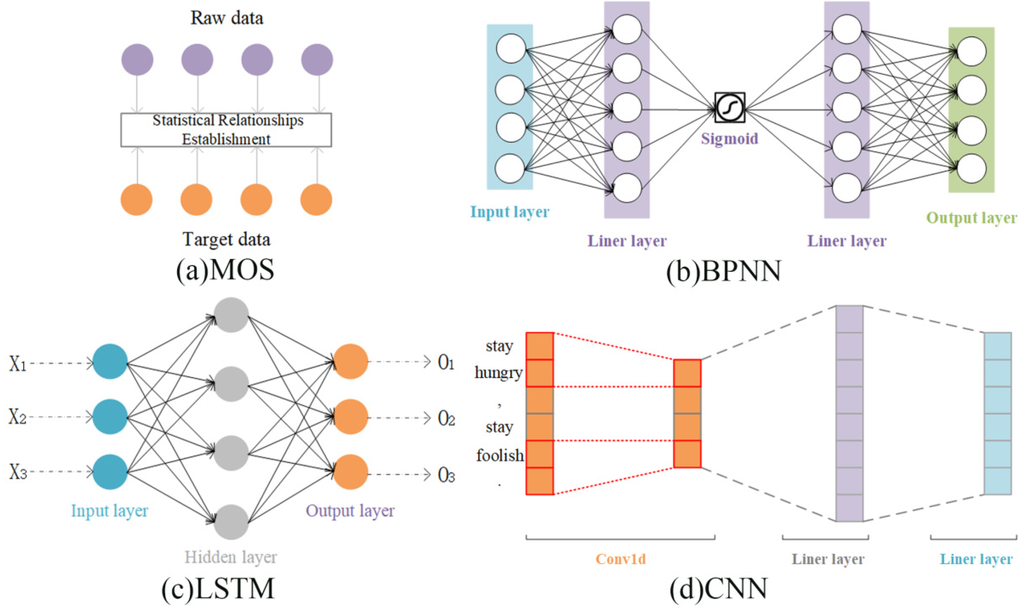
Figure 1. Schematic diagrams of the four bias correction algorithms, including (a) the Model Output Statistics (MOS) algorithm; (b) the Back Propagation Neural Network (BPNN) algorithm; (c) the Long Short-Term Memory neural network (LSTM) algorithm, and (d) the one-dimensional Convolutional Neural Network (CNN) algorithm.
Atmosphere 15 00197 g001
Figure 2. The flowchart of the established short-term ensemble forecasting model.
Atmosphere 15 00197 g002
Figure 3. The topography over the study domain used by the WRF sub-model. The areas boxed by blue lines is the domain used by the ROMS and SWAN sub-models. The black dots indicate the locations of the three buoys, and the black line connecting the little blue dots is the moving path of the Typhoon “Muifa” on 15–16 September 2022.
Atmosphere 15 00197 g003
Figure 4. The series of Buoy observations and COAWST forecasts, including (a) the series of wind speed at Laohutan (LHT) station; (b) the series of wave height at Laohutan (LHT) station; (c) the series of wind speed at Zhifudao (ZFD) station; (d) the series of wave height at Zhifudao (ZFD) station; (e) the series of wind speed at Lianyungang (LYG) station; and (f) the series of wave height at Lianyungang (LYG) station.
Atmosphere 15 00197 g004
Figure 5. The series of bias between the buoy observations and corrected forecasts using the BPNN algorithm with different data training strategies, including (a) the bias series of wind speed at Laohutan (LHT) station; (b) the bias series of wave height at Laohutan (LHT) station; (c) the bias series of wind speed at Zhifudao (ZFD) station; (d) the bias series of wave height at Zhifudao (ZFD) station; (e) the bias series of wind speed at Lianyungang (LYG) station; and (f) the bias series of wave height at Lianyungang (LYG) station.
Atmosphere 15 00197 g005
Figure 6. Box plots of bias between the forecasts and the buoy observations, including (a) box plots of the wind speed bias at Laohutan (LHT) station; (b) box plots of the wind speed bias at Zhifudao (ZFD) station; (c) box plots of the wind speed bias at Lianyungang (LYG) station; (d) box plots of the wave height bias at Laohutan (LHT) station; (e) box plots of the wave height bias at Zhifudao (ZFD) station; and (f) box plots of the wave height bias at Lianyungang station. The plots of uncorrected forecasting bias are colored in blue, the corrected bias by the MOS algorithm in green, the corrected bias by the BPNN algorithm in yellow, the corrected bias by the LSTM algorithm in black, the corrected bias by the CNN algorithm in purple, the bias of the final ensemble forecasts (ENS) in red, and the differences between the ERA5 data and observations in brown.
Atmosphere 15 00197 g006
Figure 7. The bias series from 24 h ensemble forecasts and corrected results by four algorithms, including the bias series of (a) wind speed and (b) wave height at Laohutan (LHT) station, the bias series of (c) wind speed and (d) wave height at Zhifudao (ZFD) station, and the bias series of (e) wind speed and (f) wave height at Lianyungang (LYG) station. The corrected bias by MOS is colored in green, the corrected bias by BPNN in yellow, the corrected bias by LSTM in black, the corrected bias by CNN in purple, and the bias of the final ensemble forecasts in red, and the differences between the ERA5 data and observations are represented by brown dots.
Atmosphere 15 00197 g007
Figure 8. The Taylor diagrams of the 24 h forecasts from final ensemble product and other correction result, including the diagrams of forecasted wind speed at (a) Laohutan (LHT) station, (b) Zhifudao (ZFD) station, and (c) Lianyungang (LYG) station, and the diagrams of forecasted wave height at (d) Laohutan (LHT) station, (e) Zhifudao (ZFD) station, and (f) Lianyungang (LYG) station. The dots of uncorrected forecasts are colored in blue, the dots corrected by MOS in green, the dots corrected by BPNN in yellow, the dots corrected by LSTM in black, the dots corrected by CNN in purple, the dots from final ensemble forecasts in red, and the dots from the ERA5 data in brown.
Atmosphere 15 00197 g008
Figure 9. The histograms of RMSE of forecasts with different forecasting time, including the RMSEs of (a) wind speed and (b) wave height at Laohutan (LHT) station, the RMSEs of (c) wind speed and (d) wave height at Zhifudao (ZFD) station, and the RMSEs of (e) wind speed and (f) wave height at Lianyungang (LYG) station. The three columns in the same color represent the RMSEs from the forecasts of 24 h, 48 h, and 72 h ahead, respectively. The RMSE columns of uncorrected forecasts are colored in blue, the columns corrected by MOS in green, the columns corrected by BPNN in yellow, the columns corrected by LSTM in black, the columns corrected by CNN in purple, the columns from ensemble forecasts in red, and the columns of the ERA5 data in brown.
Atmosphere 15 00197 g009
Table 1. Mean RMSEs of wind speed and wave height from the three tests with different simulation time duration.
LaohutanZhifudaoLianyungang
Wind Speed Wave HeightWind Speed Wave HeightWind SpeedWave Height
S1−1.52 m/s0.13 m−1.19 m/s0.08 m−0.91 m/s0.02 m
S2−1.67 m/s0.09 m−1.53 m/s0.09 m−0.86 m/s−0.01 m
S3−1.78 m/s0.15 m−1.76 m/s0.13 m−0.96 m/s−0.02 m
Table 2. Correlation coefficients between the buoy observations and surface variables of COAWST during the training period.
VariableApplied TestLaohutanZhifudaoLianyungang
Wind Speed Wave HeightWind Speed Wave HeightWind Speed Wave Height
T2M *wind and wave in T2 and T4−0.210.12−0.17−0.33−0.010.2
SSTwind and wave in T2 and T4−0.20.1−0.15−0.230.040.26
SLPwave in T2 and T40.05−0.240.020.34−0.050.1
RH2Mwind in T2 and T4−0.250.08−0.23−0.23−0.040.04
HFXwind in T2 and T40.24−0.010.310.70.280.26
LHwind in T2 and T40.330.140.350.580.250.33
OLRNone−0.15−0.09−0.12−0.22−0.090.09
LWAVEPwave in T2 and T40.090.470.050.30.10.41
PWAVEwave in T2 and T40.060.41−0.010.220.070.38
USTwind in T2, T3, and T4, wave in T30.540.430.530.690.670.69
PSFCwave in T2 and T40.05−0.240.020.34−0.05−0.1
GSWNone0.001−0.03−0.07−0.1−0.08−0.06
Wind Speedwind in T1, T2, T3, T4, and T5, wave in T30.550.470.530.610.670.64
HWAVEwind in T3, wave in T1, T2, T3, T4, and T50.490.720.510.730.650.8
* T2M: temperature at 2 m level; SST: sea surface temperature; SLP: sea level pressure; RH2M: relative humidity at 2 m level; HFX: upward heat flux at surface; LH: latent heat flux at surface; OLR: total outgoing long radiation; LWAVEP: wave length; PWAVE: wave period; UST: U* in similarity theory; PSFC: surface pressure; GSW: net short wave radiation flux at ground surface; Wind Speed: composed of U10 and V10 wind component at 10 m level; HWAVE: significant wave height.
Table 3. The RMSEs between buoy observations and corrected forecasts by BPNN with different training strategies.
LaohutanZhifudaoLianyungang
Wind SpeedWave HeightWind SpeedWave HeightWind SpeedWave Height
T12.03 m/s0.24 m2.20 m/s0.38 m2.07 m/s0.23 m
T22.66 m/s1.57 m2.56 m/s1.58 m2.40 m/s4.44 m
T32.22 m/s0.24 m2.20 m/s0.32 m2.08 m/s0.30 m
T42.74 m/s0.30 m2.77 m/s0.49 m2.56 m/s0.31 m
T51.99 m/s0.24 m2.20 m/s0.39 m2.14 m/s0.24 m
Table 4. The promotion values of correlation coefficients for the corrected forecasts compared with the uncorrected ones of 24 h, 48 h, and 72 h ahead.
Promotion ValueAlgorithmLaohutanZhifudaoLianyungang
Wind SpeedWave HeightWind SpeedWave HeightWind Speed Wave Height
24 h forecastsMOS−0.0030.0080.0220.0040.02−0.04
BPNN0.060.0220.0280.0070.090.1
LSTM0.0390.010.0150.010.108−0.01
CNN0.0330.0250.0180.0030.1050.007
ENS−0.007−0.01−0.04−0.020.08−0.03
48 h forecastsMOS0.003−0.0180.0100.002−0.008
BPNN0.05−0.0120.030.0080.050.012
LSTM0.03−0.00060.0002−0.0060.041−0.1
CNN0.02−0.014−0.0180.020.0430.011
ENS−0.02−0.04−0.04−0.060.005−0.048
72 h forecastsMOS0.006−0.0090.013−0.030−0.006
BPNN0.060.0160.0250.0080.040.009
LSTM0.009−0.0060.0070.010.01−0.13
CNN−0.0050.0140.0140.020.030.006
ENS−0.010−0.06−0.08−0.03−0.07
The highlighted value represents the maximum value among the four groups of corrected forecasts.
Disclaimer/Publisher’s Note: The statements, opinions and data contained in all publications are solely those of the individual author(s) and contributor(s) and not of MDPI and/or the editor(s). MDPI and/or the editor(s) disclaim responsibility for any injury to people or property resulting from any ideas, methods, instructions or products referred to in the content.