Implementation of an On-Line Reactive Source Apportionment (ORSA) Algorithm in the FARM Chemical-Transport Model and Application over Multiple Domains in Italy

Abstract

A source apportionment scheme based on gas and aerosol phase reactive tracers has been implemented in the chemical-transport model FARM, to efficiently estimate contributions of different sources to ambient concentrations. The on-line scheme deals with all the main processes that the chemical species undergo in the model, to enhance consistency with the calculation of bulk concentrations. The fate of precursors through gas-phase chemical reactions is followed by an efficient solver that determines their incremental reactivity, while the contributions to the secondary particulate species from their gaseous precursors is determined by assuming the thermodynamic equilibrium between the two phases. The paper details the new employed methodologies and illustrates the application of the apportionment scheme (based on 6 source sectors) to PM10 and O₃, simulated on three domains of different dimensions in Italy, all sharing the same horizontal resolution and a common region (Lombardy). Spatial patterns of results show, on average, a relevant contribution of heating on PM10 concentration in January, with local hotspots dominated by road traffic. Contributions appear consistent in the three simulated domains, apart from the boundary conditions, influenced by the dimension of the domain. Hourly series of contributions to O₃ concentrations in July at three selected sites show the dominance of boundary conditions, underlining the large scale of O₃ formation. Finally, for PM10 components, the resulting sectorial contributions are compared with the impacts computed via the brute force method, showing that results are similar for elemental carbon and sulfate, while they are different for nitrate and ammonium, due to a different allocation of contributions and impacts between the methods. Each approach responds in principle to a different purpose, and their combined use provides possibly a wide set of information useful for addressing the different air quality management needs.

1. Introduction

The estimation of the role of different sources in atmospheric pollution is fundamental information for the elaboration of effective air quality control plans. The European legislation requires to provide, for any annual assessment of ambient concentrations reporting exceedances of limits, an estimation of the main sources responsible for the exceedance. These estimations are usually obtained using source apportionment (SA) techniques and may be conducted either through receptor models (RM) [1,2,3] and/or dispersion models, sometimes used simultaneously, aiming for more robust results. Among dispersion models, chemical-transport models (CTMs) are mainly used [4] and the strengths and weaknesses of RM and CTMs have been extensively discussed before [5,6,7].

CTMs are modelling techniques largely used for air quality assessments since they may simulate the fate of both primary and secondary pollutants in the atmosphere through a detailed description of atmospheric physical and chemical processes using as input emission and meteorological data as well as various surface information (land-use, salinity, vegetation type, roughness, heat fluxes, temperature). SA techniques employed in CTMs may be grouped in two types of approaches: the so-called brute force methods (BFM) and tagged species methods (TAG).

The BFM quantify the sensitivity of one CTM, i.e., the response of modelled concentrations to variations in emissions and can be applied with any CTM. The variations may interest one or more sources, either by suppressing all emissions (usually referred to as the zero–out method, e.g., [8,9]) or by reducing emissions to some extent with respect to reference data [10,11,12].

This method involves multiple runs and is computationally expensive; therefore, specific algorithms have been developed to calculate CTM sensitivities simultaneously with the total (bulk) concentrations, such as the decoupled direct method DDM [13,14,15], and its extension DDM-3D [16,17]. DDM has been further extended to calculate high-order sensitivities (HDDM, [18,19,20,21]). Compared to standard CTM runs, these algorithms require additional memory space and CPU time, nevertheless allowing the SA to be significantly more efficient than the BFM, in terms of computational demand [16].

TAG methods are explicitly designed for SA purposes. By adding surrogate species, they track the pollutants emitted by a specific sector or area and follow their subsequent physical and chemical transformations in the atmosphere. Hence, the name of “reactive tracers”, through which these species are generally known, also allow us to follow the intermediate species along the chemical pathways linking emitted precursors to secondary compounds. A key aspect of these methods is constraining the sum of the concentration’s contributions from the different sources always to be equal to the total concentration due to all the sources [22]. The Ozone SA Technology (OSAT, [23]), the Particle SA Technology (PSAT, [22,24,25]) within the CAMx model, the tagged species SA algorithms within CMAQ, such as TSSA [26,27] and ISAM (Integrated SA Method, [28]), the SIA SA algorithm [21], the ozone (O₃) tagging within WRF-Chem [29,30], the UCD/CIT model SA of nitrogen oxides (NO_X), and volatile organic compounds (VOCs) [31] are some examples of TAG methods. In Europe, several tagged species methods were developed and/or applied in state-of-the-art CTMs (DEHM, [32]; LOTOS-EUROS, [33]; CMAQ-ISAM, [34]; CAMx-PSAT, [35]; WRF-Chem, [36]).

In those applications, the attribution to emission sectors was studied, being very relevant information to understand “what/who does how much”, i.e., the quantitative contributions (how much) of different human activities (what) and territorial entities (who) to concentrations.

Here a new SA tagging scheme named ORSA (On-line Reactive SA) is described, as is its implementation in the FARM (Flexible Atmospheric Regional Model) CTM (http://farm-model.org; accessed on 10 October 2023); [37,38]). The purpose of this work is precisely to test this new algorithm and provide quantitative evaluations of source sectors contributions.

FARM is the core component of the atmospheric modelling system of MINNI (National Integrated Model for International Negotiation on air quality), supporting the Italian Ministry of the Environment and Energy Security in the assessment of national air quality measures and in the international negotiation on atmospheric pollution [39,40]; it is also part of the Copernicus Atmosphere Monitoring Service (CAMS, https://atmosphere.copernicus.eu/; accessed on 10 October 2023), producing European air quality forecasts [41,42]. Furthermore, it is routinely employed by various Italian Environmental Regional Agencies as part of their institutional activities (daily forecast, annual assessment, air quality plans) [43].

The model can be configured with different gas-phase mechanisms, implemented through the KPP pre-processor [44], and different aerosol schemes. In this work, SA has been implemented on the FARM 5.1 version using the SAPRC-99 gas-phase chemical mechanism [45], the three-modal aerosol scheme of [46], ISORROPIA [47] for thermodynamic equilibrium of inorganic species, and SORGAM [48] for secondary organic aerosol formation.

The ORSA algorithm is used here for modelling experiments used to apportion simultaneously particulate matter with a diameter lower than 10 μm (PM10) and O₃. PM10 is a pollutant that has a high impact on human health and, therefore, its investigations are relevant for developing efficient air quality management plans. In Italy, to which the applications shown here refer, 49,900 premature deaths were attributed to fine particulate matter in 2019 [49] and nearly 37,000 are estimated for 2030 [50]. O₃ was also evaluated, as it is of primary concern for nowadays for the impact on ecosystems, namely in Mediterranean countries [51], and it will be difficult to abate in the near future, also due to rising temperatures implied by climate change [52]. Furthermore, PM10 and O₃ were chosen for the first evaluation of ORSA because of their complex atmospheric chemistry, involving many different precursors and, therefore, multiple emission sources. ORSA is, however, available for all pollutant species calculated by the FARM model, e.g., nitrogen dioxide (NO₂), carbon monoxide (CO), and sulfur dioxide (SO₂).

In Section 2, the ORSA algorithm is described in detail together with the setup of modelling experiments used to apportion PM10 and O₃ simultaneously. Section 3 shows the ORSA results and a comparison with the BFM approach. This evaluation was carried out over three domains: Lombardy region, North of Italy, and the whole Italy. Further discussion of results and conclusions is provided in Section 4.

2. Methodology

The ORSA tagging algorithm has been developed to track simultaneously the contributions of emission sources and the contributions of initial conditions (IC) and boundary conditions (BC) to PM10 and O₃ concentrations.

In the case of PM10, the prediction capacity of TAG methods may be also assessed through comparison with the results of RM methods, based on measurements of PM chemical compounds. These data are rarely available and usually only in a few sites for a specific period. In addition to that, the comparison of the sources identified by TAG and RM is not straightforward [4,53]. On another side, BFM and TAG methods have been compared in multiple studies, with BFM often used as a reference against which the peculiarities of other methods are analyzed [8,54,55,56]. Therefore, here the contributions of different emission sources estimated through the ORSA TAG approach have been compared to their impact (BFM approach) using the same CTM, in the same configuration and with the same input data. In the absence of non-linear physical and chemical interactions, for primary pollutants, the two approaches yield the same results [57]. This is also the case when emission reductions used by BFM are not substantial [4]. The increase in the differences between these two methods in the presence of non-linear relationships between emissions and concentrations has been examined in the methodological reviews by [58] and [7]. These studies pointed out that sensitivity analyses are more to evaluate the impact of abatement strategies, while tagged methods are more suitable to retrieve source contributions within the current emission framework [59]. Moreover, the latter ones could provide useful information for investigating model processes, and the combination of the two approaches offers valuable insights in showing the contribution of mitigated sources with respect to unmitigated ones [57].

The nomenclature we will adopt to identify the results of the two methods is “impacts” for BFM and “contributions” for TAG.

ORSA is designed to track the contribution to concentrations from different groups of sources, hereinafter referred as “source sets” (SS), using a tagged species approach that starts from [28,60]. Each SS is assigned to the model through a separate emission input, carrying a subset of the bulk emissions that are assigned for a standard model run. The atmospheric fate of the pollutants associated with the emissions from each SS is then followed through a set of reactive tracers (tags) that undergo the same physical and chemical processes of the bulk model species. Additional tags also enable tracking the contributions from the concentrations given as IC and BC to model simulation. These two inputs are treated similarly to an SS.

Tags are a fictitious construct—they are not present in the real world and cannot be measured. Nevertheless, we imagine that whenever some mass is injected into the model simulation from a particular SS, all molecules injected are tagged as originating from that SS. As soon as a chemical reaction takes place involving two molecules with different tags, the molecules produced by the reaction should carry “mixed” tags, because some of their atoms come from one SS, and some from the other one. If we wanted to be strictly consistent with our assumptions, each atom should be tagged with its originating SS tag. Mass conservation would naturally follow in that case. However, implementing this in the model code would be too complicated. Instead, we continue to attribute tags to molecules and, in order to do so, we make two assumptions: (1) “summability”, stated in Equation (2): for each chemical species, the sum of all the tag concentrations is always equal to the correspondent bulk concentration; (2) “product halving”, stated in Equation (5) and consistent with “summability”: when two reagents have different tags, say X and Y, the reaction product concentrations are split in two, so that, ideally, half of the molecules produced are assigned to tag X, and the other half to tag Y.

The evolution of the tracer species (tags) is following as much as possible the same algorithms used for the bulk species, to maximize the consistency between tracer and bulk species, avoiding code redundancy and preserving its modularity in view of future model developments. Details on the algorithms implemented for the different processes (advection–diffusion, gas-phase chemistry, ozone, aerosol processes, and cloud processes) are given in Section 2.1, while the modelling setup used for evaluation is described in Section 2.2.

2.1. Tagged Species Source Apportion Algorithms

2.1.1. Advection–Diffusion

When simulation starts, all tags (of each tagged species) are initialized to zero, except the IC tag, which is initialized with the 3D concentration field of the corresponding species assigned in the input as initial conditions. Lateral and top boundary conditions for all tags (of each tagged species) are initially set to zero, except for the BC tag: its lateral and top boundary conditions are set to the concentration values from the time-varying boundary condition fields for the corresponding species assigned in input.

Emissions from diffuse and point sources of each SS are injected into the computational grid in the same way used for bulk emissions, thus incrementing concentrations of the corresponding tag.

Advection–diffusion of tags in the three spatial directions is then simulated by the same algorithms already present in the code for bulk concentrations, and all tags are subject to the same deposition velocities of the corresponding bulk species.

2.1.2. Gas-Phase Chemistry

The chemical transformations that all gaseous species undergo can be represented by a vector differential equation:

$$\frac{dc}{dt}=\mathit{R}\left(c\right)$$

(1)

where $\mathit{c}$ is the vector storing the bulk concentrations (at current time t) of the N gaseous species and $\mathit{R}\left(\mathit{c}\right)$ is the vector of net reaction rates, a function of $\mathit{c}$. Each gaseous species is apportioned in M tracked tags, each corresponding to a source set. Tag concentrations are stored in a matrix, C, with dimensions $\left(N,M\right)$: each of its rows contains the tag concentrations of a particular species, and each of its columns, say ${\mathit{c}}_m$, contains the concentrations of all species for the m-th tag. As anticipated above, the “summability” assumption states that, for each species, the sum of all tags (i.e., the ones associated with the SS, plus IC and BC) must always be equal to the correspondent bulk concentration:

$$\sum _{m=1}^M{\mathit{c}}_m=\mathit{c}$$

(2)

Remark that this condition is imposed on tags, not on bulk concentrations, which are not affected in any way by the activation of ORSA in a FARM run. Here and in the following, indexed small letters indicate tags, whereas small letters without an index indicate bulk concentrations.

Both first-degree and second-degree terms appear in the chemical transformation equations. Without loss of generality, suppose that the equation for a particular species, $c$, depends on concentrations of species $a$, $b$, and $c$ itself in this way:

$$\frac{dc}{dt}=\sigma c+\rho ab$$

(3)

where $\sigma$ and $\rho$ do not depend on species concentrations. Write each bulk concentration as the sum of its tags:

$$\sum _{m=1}^M\frac{d{c}_m}{dt}=\sigma \sum _{m=1}^M{c}_m+\rho \left(\sum _{j=1}^M{a}_j\right)\left(\sum _{k=1}^M{b}_k\right)$$

(4)

The “product halving” anticipated above is now applied. Among second-degree terms, products of two different tags are present: we assume that such products contribute in equal measure to the evolution of both tags and, consequently, we split them in two halves (summability would not be guaranteed otherwise). Equation (4) is then re-written as:

$$\sum _{m=1}^M\frac{d{c}_m}{dt}=\sigma \sum _{m=1}^M{c}_m+\frac{1}{2}\rho \left(\sum _{m=1}^M{a}_m\right)\left(\sum _{k=1}^M{b}_k\right)+\frac{1}{2}\rho \left(\sum _{k=1}^M{a}_k\right)\left(\sum _{m=1}^M{b}_m\right)$$

(5)

The right-hand side may now be written as a sum over index m:

$$\sum _{m=1}^M\frac{d{c}_m}{dt}=\sum _{m=1}^M\left[\sigma c_m+\frac{1}{2}\rho a_m\left(\sum _{k=1}^M{b}_k\right)+\frac{1}{2}\rho \left(\sum _{k=1}^M{a}_k\right)b_m\right]$$

(6)

We impose that the equality holds for each term of the sum to obtain the evolution equation for tag m of species $c$:

$$\frac{d{c}_m}{dt}=\sigma c_m+\frac{1}{2}\rho {ba}_m+\frac{1}{2}\rho a{b}_m$$

(7)

where $a$ and $b$ (without index) are bulk concentrations (evolving as in an ordinary FARM run). Remark that Equation (7) is not an approximation, since the constraint defined by Equation (2) guarantees a free choice of the tagged components $c_m$, provided that the summability assumption is ensured. This is simply equivalent to considering each tracer evolving separately from each other, in the common background of bulk species, $a$ and $b$, determined by the whole emission inventory.

We observe that tag-multiplying coefficients on the right-hand side of Equation (7) show some resemblance to derivatives of terms appearing in the bulk evolution equation, Equation (1), i.e., the components of the Jacobian matrix J of the vector function $\mathit{R}$:

$$J_{i,k}\equiv \frac{\partial R_i}{\partial c_k}$$

(8)

In the example of Equations (3)–(7), the row of the Jacobian matrix corresponding to species $c$ is, in fact, as follows:

$${\mathit{J}}_c=\left[\begin{array}{ccc}\rho b& \rho a& \sigma \end{array}\right]$$

(9)

Since in Equation (1) both first and second-degree terms appear, the components of the Jacobian matrix $\mathit{J}$ are either constants, i.e., zero-degree terms ($\sigma$), or first-degree terms ($\rho b$, $\rho a$) in bulk concentrations. In general, such a matrix can be written as the sum of two matrices, ${\mathit{J}}_0$ and ${\mathit{J}}_{\mathsf{1}}$, having, respectively, zero-degree and first-degree components only and zero elsewhere:

$$\mathit{J}={\mathit{J}}_0+{\mathit{J}}_{\mathsf{1}}$$

(10)

Consider now the matrix $\tilde{\mathit{J}}$, having the same components of the Jacobian matrix $\mathit{J}$, but where first-degree terms are halved:

$$\tilde{\mathit{J}}={\mathit{J}}_0+\frac{1}{2}{\mathit{J}}_{\mathsf{1}}$$

(11)

The general form of Equation (7) is written by making use of this matrix $\tilde{\mathit{J}}$ rather than the Jacobian matrix $\mathit{J}$:

$$\frac{d}{dt}\mathit{C}=\tilde{\mathit{J}}\mathit{C}$$

(12)

This is the tag (source set) evolution equation, which preserves summability by construction. In [28], the authors instead assume that the evolution of the apportionment through the gaseous phase reactions is described by:

$$\frac{d}{dt}\mathit{C}=\mathit{J}\mathit{C}$$

(13)

with the Jacobian matrix $\mathit{J}$ instead of $\tilde{\mathit{J}}$. Equation (13), though, violates the summability assumption, stated in Equation (2), by doubling the contribution of terms containing the product of different tags. With reference to the example:

$$\sum _{m=1}^M\left[\begin{array}{ccc}\rho b& \rho a& \sigma \end{array}\right]\left[\begin{array}{c}{a}_m\\ b_m\\ c_m\end{array}\right]=\sigma c+2\rho ab\ne \sigma c+\rho ab$$

(14)

From this point on, we follow the approach of Kwok et al. (2013) and make use of the following discretization [17]:

$${\mathit{C}}_{\mathit{t}+\mathit{\Delta }\mathit{t}}={\left(\mathit{I}-\frac{\mathsf{\Delta }t}{2}\widehat{\mathit{J}}\right)}^{-1}\left(\mathit{I}+\frac{\mathsf{\Delta }t}{2}\widehat{\mathit{J}}\right){\mathit{C}}_t$$

(15)

where $\mathsf{\Delta }t$ is the synchronization time step, $\mathit{I}$ is the identity matrix, and the matrix $\widehat{\mathit{J}}$ is obtained by calculating $\tilde{\mathit{J}}$ (defined in Equation (11)) on the average of bulk concentrations before (at time $\left(t\right)$) and after (at time $\left(t+\mathsf{\Delta }t\right)$) the application of the chemical solver:

$$\widehat{\mathit{J}}=\tilde{\mathit{J}}\left[\frac{\mathit{c}\left(t\right)+\mathit{c}\left(t+\mathsf{\Delta }t\right)}{2}\right]={\mathit{J}}_0+\frac{1}{2}{\mathit{J}}_1\left[\frac{\mathit{c}\left(t\right)+\mathit{c}\left(t+\mathsf{\Delta }t\right)}{2}\right]$$

(16)

An advantage of this scheme is that $\widehat{\mathit{J}}$ only depends on bulk concentrations and not on the tagged quantities, and it needs to be calculated only once for each synchronization time step $\mathsf{\Delta }t$, which is usually a multiple of the substantially smaller time step of the chemical solver. A Rosenbrock solver [44] is the preferred one currently used in FARM, but it should be noted that the present scheme does not depend on the chosen chemical solver. As in the case of the production and destruction terms appearing in the chemical differential equations, the code for Jacobian terms calculation is also generated through the KPP interpreter [44]. The terms of the above solution for tags are efficiently computed through sparse algebra subroutines also generated by KPP.

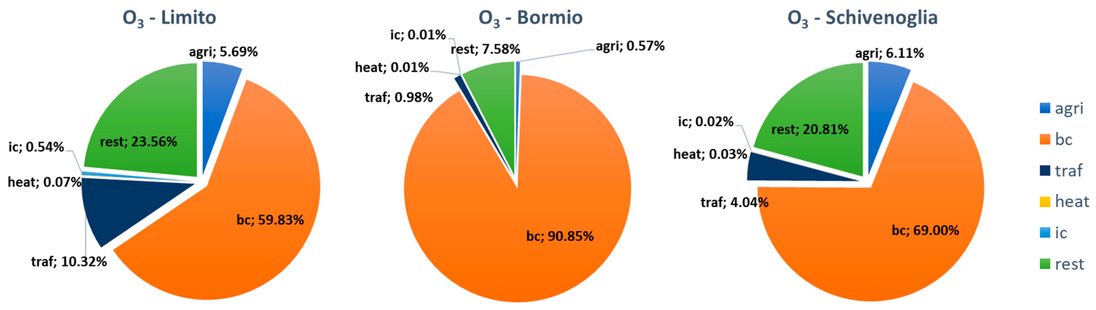
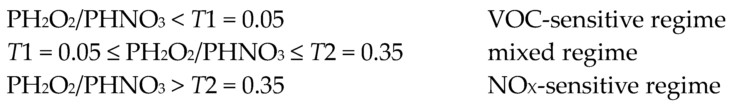
2.1.3. Specific Algorithms for O₃

The linearization involved in updating the SA for all species through the gas-phase chemical reactions, Equation (15), is too crude an approximation for O₃, so for this species, a specific algorithm has been implemented. The apportionment of O₃ production is attributed either to tags of VOC (Volatile Organic Compounds) species or to tags of nitrogen oxides (NO_X = NO + NO₂), depending on the dominating O₃ production regime. As currently assumed, e.g., by [60,61], the dominating O₃ production regime is inferred through an indicator, the ratio between the production rate of hydrogen peroxyde (H₂O₂) and that of nitric acid (HNO₃), indicated as PH₂O₂/PHNO₃ (Scheme 1). Both the numerator and denominator of this ratio are calculated by using only the positive terms appearing on the right-hand side of the differential equations of the chemical reaction scheme of the model for the two species. Consistently with what is done for the Jacobian in Equation (16), these terms are evaluated on the average of bulk concentrations before and after the application of the chemical solver.

The thresholds T1 and T2 have been defined by taking into consideration the study by [62] and the discussion by [61].

The implementation of the O₃ apportionment algorithm using the above approach requires the definition in the code of two supplementary arrays of tag concentrations for O₃: O₃N and O₃V, tracking the formation of O₃ in NO_X-sensitive ad VOC-sensitive conditions, respectively.

First, the O₃ bulk concentration net increment is calculated:

$$D\mathrm{O}3={\mathrm{O}3}^{NEW}-{\mathrm{O}3}^{OLD}$$

(17)

where ${\mathrm{O}3}^{OLD}$ and ${\mathrm{O}3}^{NEW}$ are the bulk O₃ concentrations before and after the application of the chemical solver.

When $DO3>0$, O₃ production occurs and the value of the indicator PH₂O₂/PHNO₃ is used to determine the dominating production regime. When PH₂O₂/PHNO₃ > T2, the production regime is NO_X-sensitive and

$$\begin{gathered} {\mathrm{O}3\mathrm{N}}_m^{NEW}={\mathrm{O}3\mathrm{N}}_m^{OLD}+D\mathrm{O}3 \frac{{\mathrm{N}\mathrm{O}}_m^{OLD}+{\mathrm{N}\mathrm{O}2}_m^{OLD}}{{\sum }_k({\mathrm{N}\mathrm{O}}_k^{OLD}+{\mathrm{N}\mathrm{O}2}_k^{OLD})} \\ {\mathrm{O}3\mathrm{V}}_m={\mathrm{O}3\mathrm{V}}_m^{OLD} \end{gathered}$$

(18)

where m and k are tag (source set) indexes. When PH₂O₂/PHNO₃ < T1 = 0, the production regime is VOC-sensitive and

$$\begin{gathered} {\mathrm{O}3\mathrm{N}}_m={\mathrm{O}3\mathrm{N}}_m^{OLD} \\ {\mathrm{O}3\mathrm{V}}_m^{NEW}={\mathrm{O}3\mathrm{V}}_m^{OLD}+D\mathrm{O}3 \frac{{\sum }_s({\mathrm{V}\mathrm{O}\mathrm{C}}_{s,m}^{OLD}\times {\mathrm{M}\mathrm{I}\mathrm{R}}_s)}{{\sum }_k{\sum }_s({\mathrm{V}\mathrm{O}\mathrm{C}}_{s,k}^{OLD}\times {\mathrm{M}\mathrm{I}\mathrm{R}}_s)} \end{gathered}$$

(19)

where the index s refers to each VOC species involved in O₃ production and MIRs are Maximum Incremental Reactivities, as calculated and tabulated by [45]. When T1 ≤ PH2O2/PHNO3 ≤ T2 = 0, the O₃ production regime is considered “mixed” and

$$\begin{gathered} {\mathrm{O}3\mathrm{N}}_m^{NEW}={\mathrm{O}3\mathrm{N}}_m^{OLD}+\alpha D\mathrm{O}3 \frac{{\mathrm{N}\mathrm{O}}_m^{OLD}+{\mathrm{N}\mathrm{O}2}_m^{OLD}}{{\sum }_k({\mathrm{N}\mathrm{O}}_k^{OLD}+{\mathrm{N}\mathrm{O}2}_k^{OLD})} \\ {\mathrm{O}3\mathrm{V}}_m^{NEW}={\mathrm{O}3\mathrm{V}}_m^{OLD}+\left(1-\alpha \right) D\mathrm{O}3 \frac{{\sum }_s({\mathrm{V}\mathrm{O}\mathrm{C}}_{s,m}^{OLD} {\times \mathrm{M}\mathrm{I}\mathrm{R}}_s)}{{\sum }_k{\sum }_s({\mathrm{V}\mathrm{O}\mathrm{C}}_{s,k}^{OLD}\times {\mathrm{M}\mathrm{I}\mathrm{R}}_s)} \\ \mathrm{w}\mathrm{h}\mathrm{e}\mathrm{r}\mathrm{e} \hspace{1em}\alpha \equiv \frac{\frac{\mathrm{P}{\mathrm{H}}_2{\mathrm{O}}_2}{\mathrm{P}\mathrm{H}\mathrm{N}{\mathrm{O}}_3}-T_1}{T_2-T_1} \end{gathered}$$

(20)

Finally, when the net increment is negative, $D\mathrm{O}3<0$, O₃ destruction occurs and is estimated as follows:

$$\begin{gathered} {\mathrm{O}3\mathrm{N}}_m^{NEW}={\mathrm{O}3\mathrm{N}}_m^{OLD}+D\mathrm{O}3 \frac{{\mathrm{N}\mathrm{O}}_m^{OLD}+{\mathrm{N}\mathrm{O}2}_m^{OLD}}{{\sum }_k({\mathrm{N}\mathrm{O}}_k^{OLD}+{\mathrm{N}\mathrm{O}2}_k^{OLD})+{\sum }_k{\sum }_s{\mathrm{V}\mathrm{O}\mathrm{C}}_{s,k}^{OLD}} \\ {\mathrm{O}3\mathrm{V}}_m^{NEW}={\mathrm{O}3\mathrm{V}}_m^{OLD}+D\mathrm{O}3 \frac{{\sum }_s{\mathrm{V}\mathrm{O}\mathrm{C}}_{s,m}^{OLD}}{{\sum }_k({\mathrm{N}\mathrm{O}}_k^{OLD}+{\mathrm{N}\mathrm{O}2}_k^{OLD})+{\sum }_k{\sum }_s{\mathrm{V}\mathrm{O}\mathrm{C}}_{s,k}^{OLD}} \end{gathered}$$

(21)

For all three sensitive regimes, after updating the arrays O₃N and O₃V, their sum is taken as the updated tag array for O₃:

$${\mathrm{O}3}_m^{NEW}={\mathrm{O}3\mathrm{N}}_m^{NEW}+{\mathrm{O}3\mathrm{V}}_m^{NEW}$$

(22)

The O₃ apportionment is updated (by means of the specific algorithm described here) before updating the apportionment of the other species. Since O³ also enters the gas mechanism as a reagent, its influence on the apportionment of other species must be considered. The general gas-phase apportionment algorithm described above has thus been modified, so that O₃ tags enter it as constants, rather than variables. The differential equation for the update of tag m is a column of Equation (12):

$$\frac{d{\mathit{c}}_m}{dt}=\tilde{\mathit{J}}{\mathit{c}}_m$$

(23)

where $\tilde{\mathit{J}}$ is the matrix defined in Equation (11) and the vector ${\mathit{c}}_m$ contains the concentrations of the m-th tag of all species. Without loss of generality, suppose that the O₃ is the last component. Then

$${\mathit{c}}_m=\left[\begin{array}{c}{\mathit{b}}_m\\ o_m\end{array}\right]$$

(24)

and

$$\tilde{\mathit{J}}=\left[\begin{array}{cc}\tilde{\mathit{X}}& \mathit{y}\\ {\mathit{w}}^T& z\end{array}\right]$$

(25)

where the last row and column correspond to O₃ components of the matrix: $\widehat{\mathit{X}}$ is the matrix obtained by excluding from $\widehat{\mathit{J}}$ both the row and the column corresponding to O₃; $\widehat{\mathbf{y}}$ is the column of $\widehat{\mathit{J}}$ corresponding to O₃, with the exclusion of its diagonal (i.e., O₃—O₃) element, $z$, and $\mathit{w}$ is the row of $\widehat{\mathit{J}}$ corresponding to O₃, with the exclusion of its diagonal (i.e., O₃—O₃) element. The differential equation is then:

$$\frac{d}{dt}\left[\begin{array}{c}{\mathit{b}}_m\\ o_m\end{array}\right]=\left[\begin{array}{cc}\tilde{\mathit{X}}& \mathit{y}\\ {\mathit{w}}^T& z\end{array}\right]\left[\begin{array}{c}{\mathit{b}}_m\\ o_m\end{array}\right]$$

(26)

The last row must be neglected because O₃ tags have already been updated by means of the O₃ specific algorithm. The evolution of the m-th tag of all other species is

$$\frac{d}{dt}{\mathit{b}}_m=\tilde{\mathit{X}}{\mathit{b}}_m+\mathit{y}{o}_m$$

(27)

where the influence of O₃ as a reagent on other species has been put into evidence. By applying the same discretization of Equation (16), the solution is obtained as follows:

$${\mathit{b}}_m^{t+\mathsf{\Delta }t}={\left(\mathit{I}-\frac{\mathsf{\Delta }t}{2}\widehat{\mathit{X}}\right)}^{-1}\left[\left(\mathit{I}+\frac{\mathsf{\Delta }t}{2}\widehat{\mathit{X}}\right) {\mathit{b}}_m^t+\frac{\mathsf{\Delta }t}{2}\widehat{\mathit{y}} \left(o_m^t+o_m^{t+\mathsf{\Delta }t}\right)\right]$$

(28)

where $o_m^t$ and $o_m^{t+\Delta t}$ are the O₃ m-th tag concentrations, respectively, before and after the specific O₃ apportionment update.

Equation (28) can be solved by using the KPP-generated arrays and subroutines, modified as follows:

• The row and column corresponding to O₃ in the matrix $\left(\mathit{I}-\frac{\mathsf{\Delta }t}{2}\widehat{\mathit{J}}\right)$ are set to zero (except the diagonal element, which is set to one, i.e., the diagonal element of $\mathit{I}$), whereas the matrix $\left(\mathit{I}+\frac{\mathsf{\Delta }t}{2}\widehat{\mathit{J}}\right)$ remains the same, because $\widehat{\mathit{y}}$ (its O₃ column) is needed in Equation (28).
• For each tag m, $o_m^t$ (the O₃ component of ${\mathit{c}}_m^t$) is substituted with the sum $\left(o_m^t+o_m^{t+\mathsf{\Delta }t}\right)$.
• The solution for all species is then obtained by means of KPP subroutines.
• The O₃ component of the solution is finally replaced with $o_m^{t+\Delta t}$, previously obtained by means of the O₃ specific algorithm.

2.1.4. Aerosol Processes

Secondary particulate species and their precursor gases are apportioned assuming thermodynamic equilibria between the two phases [28,47,48]. The updated concentrations of the tags in the two phases are computed as the product between the updated concentrations of the corresponding bulk species and the ratio between total (precursor+aerosol) tag concentration and total (precursor+aerosol) bulk concentration at the beginning of the time step:

$$\begin{gathered} C_m^{precursor}\left(t+\mathsf{\Delta }t\right)=C^{precursor}\left(t+\mathsf{\Delta }t\right)\frac{C_m^{precursor}\left(t\right)+C_m^{aerosol}(t)}{C^{precursor}\left(t\right)+C^{aerosol}(t)} \\ {C}_m^{aerosol}\left(t+\mathsf{\Delta }t\right)=C^{aerosol}\left(t+\mathsf{\Delta }t\right)\frac{C_m^{precursor}\left(t\right)+C_m^{aerosol}(t)}{C^{precursor}\left(t\right)+C^{aerosol}(t)} \end{gathered}$$

(29)

where m is the tag index, un-indexed $C$ indicates bulk concentration, $\left(t+\mathsf{\Delta }t\right)$ and $\left(t\right)$refer to updated and un-updated quantities at current time t. For the aerosol module currently implemented, the above equations are applied to sulfate with sulfuric acid as a precursor, to nitrate with the sum of HNO₃ and nitrogen pentoxide (N₂O₅) as precursors, and to ammonium (NH₄) with ammonia (NH₃) as a precursor. In the case of organic aerosol, the corresponding precursors are summed while weighted with their aerosol yields [48]. In case of a biogenic secondary aerosol, the precursors are isoprene and monoterpenes, while in case of an anthropogenic secondary aerosol, the precursors are low volatile condensation products of alkanes, alkenes, cresols, and aromatics.

2.1.5. Cloud Processes

Aqueous phase SO₂ oxidation to SO₄ is currently described according to [63]. Their respective (bulk) concentrations are updated using

$$\begin{gathered} {SO4}^{NEW}=\gamma {SO2}^{OLD} \\ {SO2}^{NEW}={SO2}^{OLD}-{SO4}^{NEW} \end{gathered}$$

(30)

where $\gamma$ depends on the temperature, pressure, liquid water fraction, and concentrations of H₂O₂ and O₃.

The apportionment of SO₂ and SO₄ into source sets is then obtained in the same, proportional way. Tag concentrations are updated through

$$\begin{gathered} {SO4}_m^{NEW}=\gamma {SO2}_m^{OLD} \\ {SO2}_m^{NEW}={SO2}_m^{OLD}-{SO4}_m^{NEW} \end{gathered}$$

(31)

where m denotes the tag index of each species. In this way, the summability of tags with respect to bulk concentrations is preserved.

Wet deposition of tracer species is updated on the basis of the tag-to-bulk concentrations ratio, applied to the deposition of bulk species [28]:

$${WD}_m\left(t+\mathsf{\Delta }t\right)={WD}_m\left(t\right)+WD\left(t+\mathsf{\Delta }t\right)\frac{C_m\left(t\right)}{C\left(t\right)}$$

(32)

where ${WD}_m\left(t+\mathsf{\Delta }t\right)$ and ${WD}_m\left(t\right)$ are, respectively, the updated and current wet deposition of tag m, $WD\left(t+\mathsf{\Delta }t\right)$ is the updated wet deposition of the corresponding bulk species, and $C_m\left(t\right)$ and $C\left(t\right)$ are, respectively, the tag and bulk species concentrations at current time t.

2.2. Modelling Setup

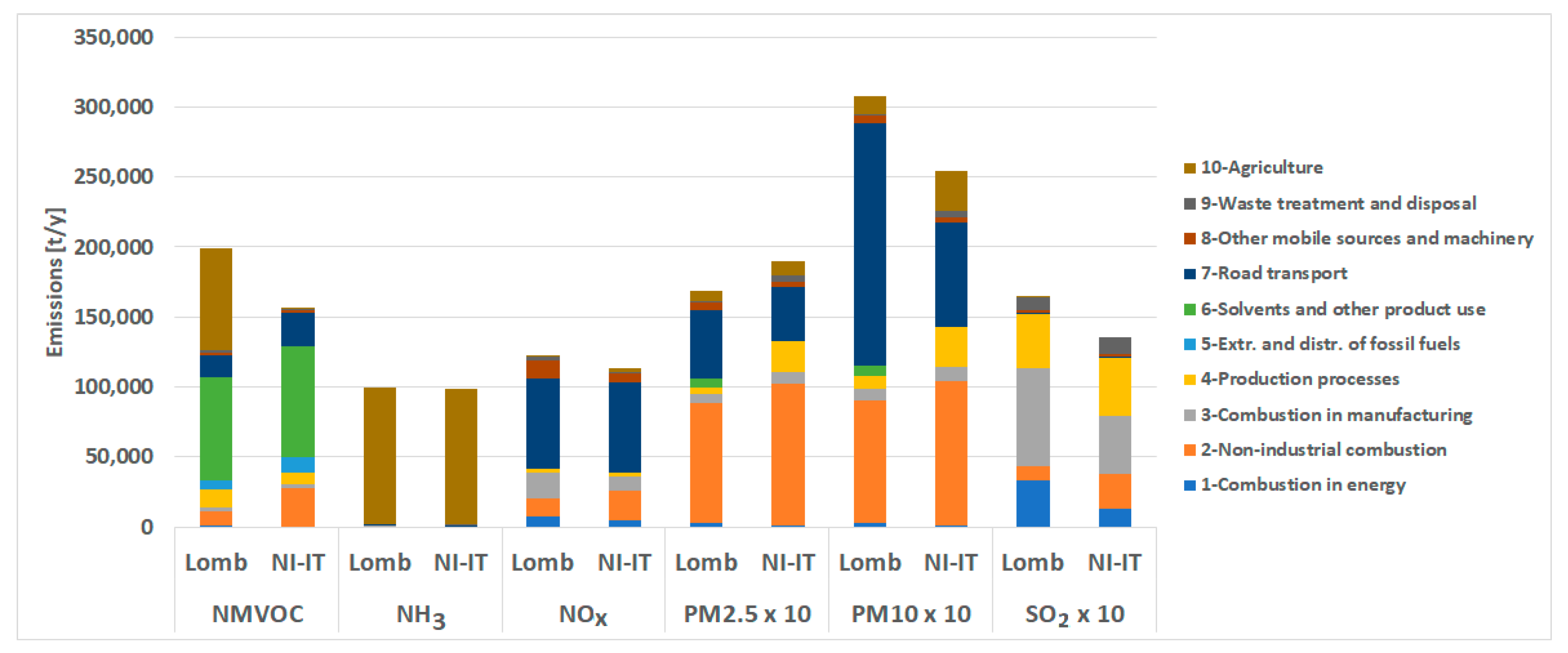
The FARM/ORSA model was applied to three domains of increasing size, located in Italy, all subdivided by grids with 4 km horizontal resolution (Figure 1). The first one (LOMB) is 256 × 244 km wide (64 × 61 grid cells), centered on the Lombardy region, and including part of the Po Valley, the Alps, and their foothills. The second one (NI) is 560 × 400 km wide (140 × 100 grid cells), and covers all Northern Italy and a portion of the surrounding countries, including all of the Po Valley, surrounded by the Alps and the Northern part of the Apennines range. Within both domains, there are zones with very diverse anthropogenic pressures, ranging from the less inhabited areas in the Alps to Milan and Turin metropolitan areas and several other smaller cities, with different types of sources giving rise to a range of atmospheric chemical regimes. The third domain (IT) is 1112 × 1232 km wide (278 × 308 grid cells) and covers all Italy. All grids share the same vertical structure, with 16 levels increasingly spaced upward from the ground, placed at 20, 65, 125, 210, 325, 480, 690, 975, 1360, 1880, 2580, 3525, 4805, 6290, 7790, 9290 m above the orography.

The configuration of the three simulation grids was chosen to investigate over a portion of the territory (i.e., the Lombardy region) the consistency of the behavior of the apportionment algorithm over domains of different size, with special regard to the computed sources’ contributions and the influence of the boundary conditions.

While the tests over the three domains (LOMB, NI, and IT) were conducted over different time periods (see Section 2.2.2), the chemical boundary conditions employed were derived from simulations on wider areas, performed using the same CTM, FARM, and the same national and pan-European emission inventories. This choice allowed us to preserve, in the LOMB simulation, the greater detail of information on emissions available in the inventory of the Lombardy region. Nevertheless, over Lombardy, the emission datasets of LOMB and NI-IT simulations are rather consistent in terms of total quantities and sectorial distributions (Figure 2), with few exceptions (e.g., NMVOC (Non-Methane Organic Volatile Compounds) from agriculture) marginally affecting the test runs that were performed. These consistencies, together with the common horizontal resolution and vertical grid adopted, allowed us to compare the apportionment results obtained for all three domains.

2.2.1. Emissions

In the following text, Italian toponymy is used, which can be interpreted using maps commonly available on the web (e.g., on https://www.worldatlas.com/maps/italy; accessed on 10 October 2023).

The emission input was prepared starting from the data of the following inventories:

• For LOMB, the regional inventory of ARPA (Regional Environmental and Protection Agency) Lombardy for the year 2012 [64], describing emission sources at the municipality level (EU NUTS 4 territorial units);
• For NI and IT, the ISPRA (Italian Institute for Environmental Protection and Research) Italian inventory for the year 2015 [65], disaggregated on provinces (EU NUTS3 territorial units) and, for the portions of the surrounding countries inside the domains, the European TNO-MACC_III inventory, the updated version of TNO-MACC_II [66].

The model-ready emission input was then prepared combining information from the cited inventories through Emission Manager [67], a modular emission pre-processing system performing:

• The speciation of organic compounds and particulate matter, based on typical profiles of each activity;
• The disaggregation on the calculation grid, with the aid of thematic spatial proxies;
• The temporal modulation with hourly resolution using annual, weekly, and daily profiles typical of each activity.

All of these lead to an hourly emission input on the three calculation grids considered.

Emission inputs were prepared considering all sources within each domain as well as selecting only the sources associated with the different sets considered in the apportionment runs on a sectorial level.

All the natural emissions (sea salt, dust, and biogenic) were determined by means of the SURFPRO 3.3 (SURFace-atmosphere interface Processor, http://doc.aria-net.it/SURFPRO/wiki/WikiStart#no1; accessed on 10 October 2023) meteorological post-processor; the MEGAN 2.04 model [68] was used for the calculation of biogenic emissions on all domains.

Table 1. Source sets (SS) considered in sectorial contribution analysis.

Source Set	Corresponding SNAP Categories
Heating	2—Non-industrial combustion
Road traffic	7—Road transport
Agriculture	10—Agriculture 8.6—Other moving sources and machinery—Agriculture
Rest	1—Energy production and fuel transformation 3—Combustion in industry 4—Production processes 5—Extraction and distribution of fuels 6—Use of solvents 8—Other moving sources and machinery (excluding agriculture) 9—Treatment and disposal of waste (other sources) 11—Natural sources

shows the four sets of anthropogenic activities/sectors considered in testing ORSA, with an indication of the corresponding broad first-level categories of EU SNAP classification (Selected Nomenclature for sources of Air Pollution; [69]) used by the emission inventories.

ORSA also takes into account two additional SSs: the impacts of BC and IC. A total of six SSs were then considered for the three domains.

The choice of the SSs was driven by their relevance to the total primary emissions of PM and O₃ precursors in Lombardy. For PM and NO_X emissions, heating and road traffic are largely prevalent on the other sectors, while NH₃ is emitted mostly by agriculture. NMVOC and SO₂ are also precursors with prevalent source contributions (solvents, combustion in manufacturing, production processes), but these were not considered as individual SSs. The reason was both to reduce the computational effort in the various tests of the apportionment scheme and to focus on the chemistry of NO_X-NH₃, which is known as a main concern in studies of the impacts/contributions on the Po Valley [53,70,71].

2.2.2. Boundary Conditions and Meteorological Input

For LOMB, the meteorological input and chemical boundary conditions for the year 2010 were prepared from the 12 km horizontal resolution fields produced by the QualeAria system (www.qualearia.it; accessed on 10 October 2023; [72]), based on the RAMS and FARM models. RAMS [73] meteorology was downscaled using the SWIFT diagnostic model [74] accounting for the orography and land-use (EEA Corine Land Cover; [75]) of the target grid, while chemical boundary conditions were prepared from FARM outputs at 12 km resolution.

For the year 2015, the meteorological input for NI simulation was prepared remapping the three-dimensional outputs of the IT domain of the MINNI 2015 simulation for Italy [76]. CAMS-global fields [77] were used for initial (IC) and boundary (BC) conditions for the MINNI run; the WRF model [78] was used to produce the meteorological forcing (data assimilation through spectral nudging (nx = 6, ny = 5) was applied).

2.2.3. Computing Architecture

The ORSA scheme has been implemented so far for single-grid model runs. The sources making up an SS can correspond either to one or multiple activity sectors, sources related to given geographic entities (e.g., administrative entities), or a combination of both. Emissions from each SS are put in a separate couple of emission files (one for gridded and one for point sources), counterparts of the input files used to assign to the model the bulk emissions from all sources within the domain. Thus, the model, in addition to the emission input files of a standard non-apportionment run, receives additional input, that is a number of input file pairs (diffuse and point emissions) equal to the number of SS chosen by the user. Standard and SS emission inputs are prepared through the same emission pre-processing system. This setup of SS allows great flexibility in subdividing sources by sectors and geographic entities, and consequently to perform apportionment runs according to different needs.

The algorithms tracking the tags through the different processes have also been implemented by adhering to the parallelization paradigms already available within the code [79]: OpenMP, MPI, and hybrid (combining the two previous ones). This allows us to efficiently run the code in SA mode on machines with different architectures, ranging from a single multi-core processor to larger clusters, as in the case of the tests illustrated in the following section.

Here are some examples of CPU time spent on different machines. FARM runs on the two larger domains (IT and NI) and 6 SSs have been performed on an ENEA CRESCO6 high performance computing grid [80], with Intel 8160 CPU nodes (Intel^® Xeon^® Platinum 8160 CPU @ 2.10 GHz, 48 cpu/node, max. memory/swap/tmp 191.6/19.5/86.0 GB). LOMB simulations have been performed on a smaller cluster with 2 nodes (Intel^® Xeon^® E5-2695v4 2.10 GHz, 18 cpu/node, max memory 64 GB). The FARM code has been compiled with Intel Fortran.

Regarding IT simulations, a hybrid MPI-OpenMP executable has been used, with MPI flavor IMPI-Intel17, employing 2 nodes and 96 cores (24 OMP × 4 MPI) for each run, resulting in a 4 h/day elapsed time. For the NI and LOMB domain, an OpenMP executable has been run with 48 and 32 threads, respectively, resulting in a 0.5 h/day and about 9 min/day elapsed time, respectively.

Concerning the computational effort with respect to BFM, the runs on the LOMB domain showed that a single FARM-ORSA run, with 6 SSs, required about 70% of the CPU time required by 6 individual runs of a BFM application, with considerably simpler management of inputs and outputs.

3. Application and Evaluation

3.1. Validation of Simulations

The results of simulations on the three domains were validated against the observations from EEA-EIONET (European Environment Information and Observation Network, http://cdr.eionet.europa.eu/en/eu/aqd/e1a/; accessed on 10 October 2023) available for each of them. On each domain, the input meteorological data and the air quality observations belong to the same year. Emissions were used for the same meteorological year, if the official emission inventory was available, or from the closest one available. The latter is the case of the 2012 regional inventory used for the simulation on the LOMB domain, which refers to the year 2010. The measurements of 2010 are used for LOMB, while the measurements of 2015 are used for NI and IT. Figures S1–S3, in the Supplementary Material (SM), show the global performances for all background stations as distributions arranged in box plots and whiskers.

Since there is no single or set of best-measure indicators [81] for the analysis of model performances, here a combination of indicators was considered: fractional bias (FB), normalized mean square error (NMSE), and Pearson correlation (CORR). These statistical indicators give an overview of model performances in reproducing bulk concentrations for the months of January and July, which are intended as representative of winter and summer periods, respectively. In

Table 2. Indicators used to evaluate model performance (M = model data, O = observed data, N = number of observations).

Fractional bias (FB)	$B=\raisebox{1ex}{$1$}\!\left/ \!\raisebox{-1ex}{$N$}\right.\ast \left(\frac{\sum _{i=1}^N(M_i - O_i)}{\sum _{i=1}^N\left(\frac{(M_i + O_i)}{2}\right)}\right)$
Correlation (R)	$R={\sum }_{i=1}^N\left(M_i-\overline{M}\right)\left(O_i-\overline{O}\right)/{\sigma }_c{\sigma }_o$
Normalized mean square error (NMSE)	$NMSE=\frac{1}{\overline{M}}\ast \sqrt{\frac{1}{N}{\displaystyle \sum _{i=1}^N}{(M_i-O_i)}^2}$

, the error statistics considered in this work are shown. The benchmarks shown are similar to those of other models in the literature [82,83].

3.2. Sector Contributions

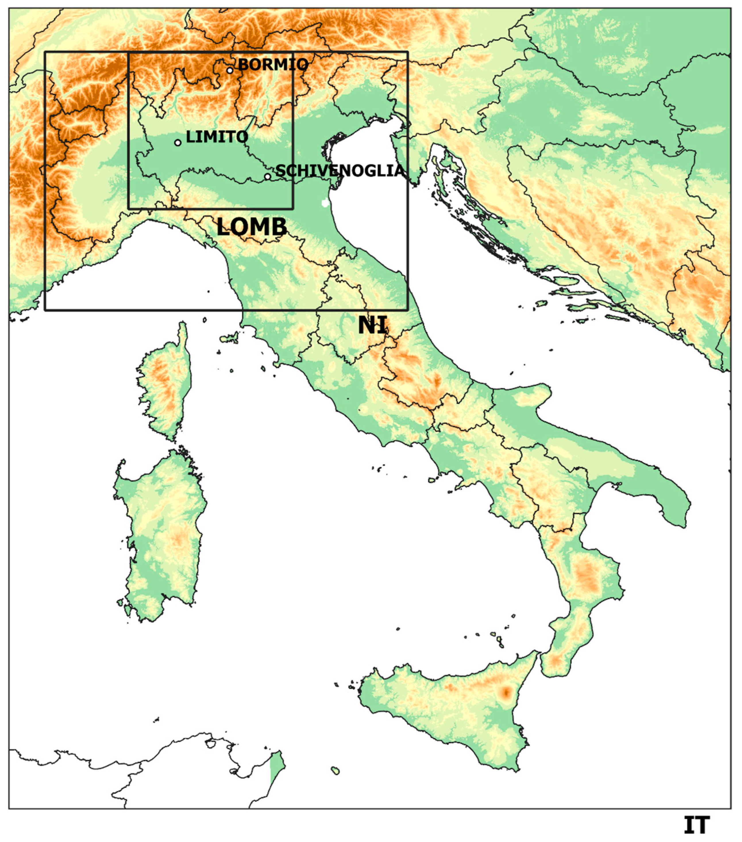
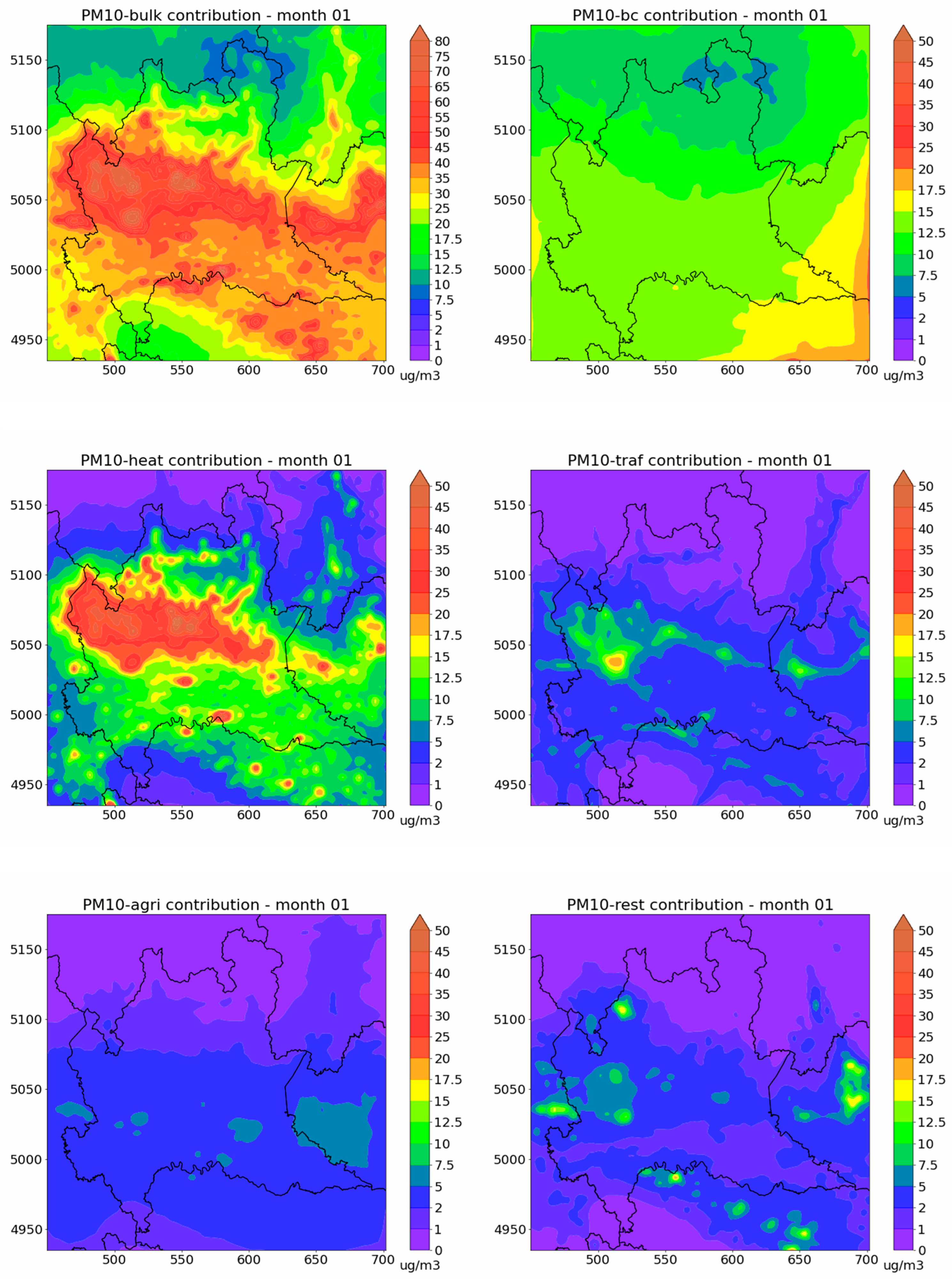
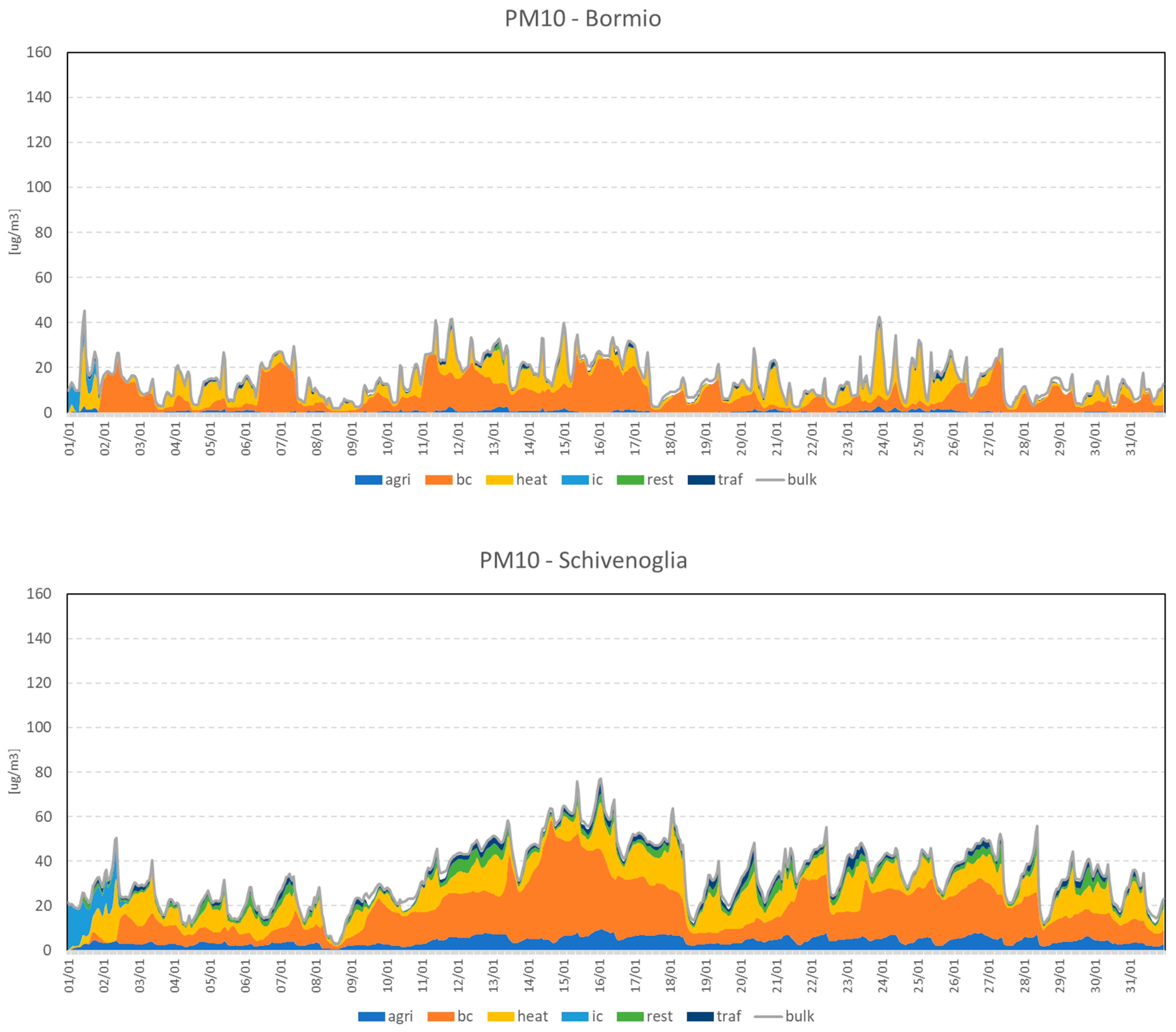
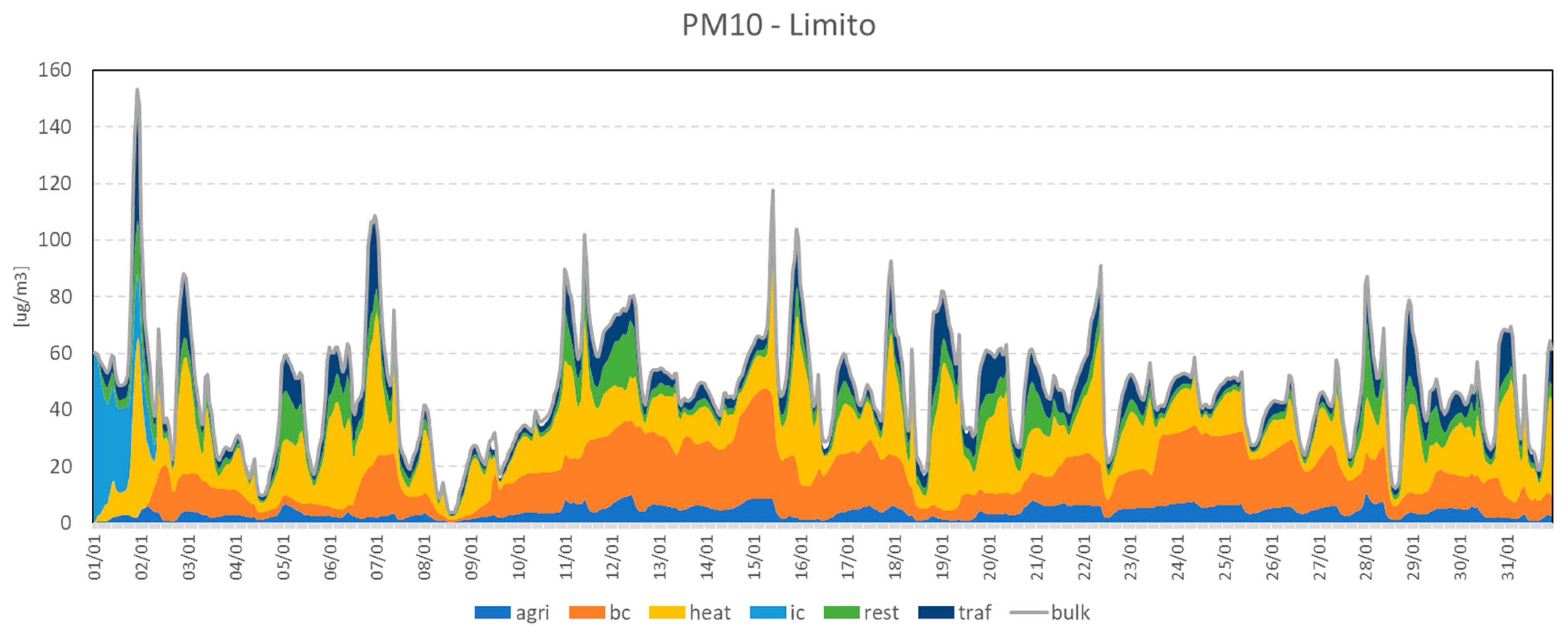
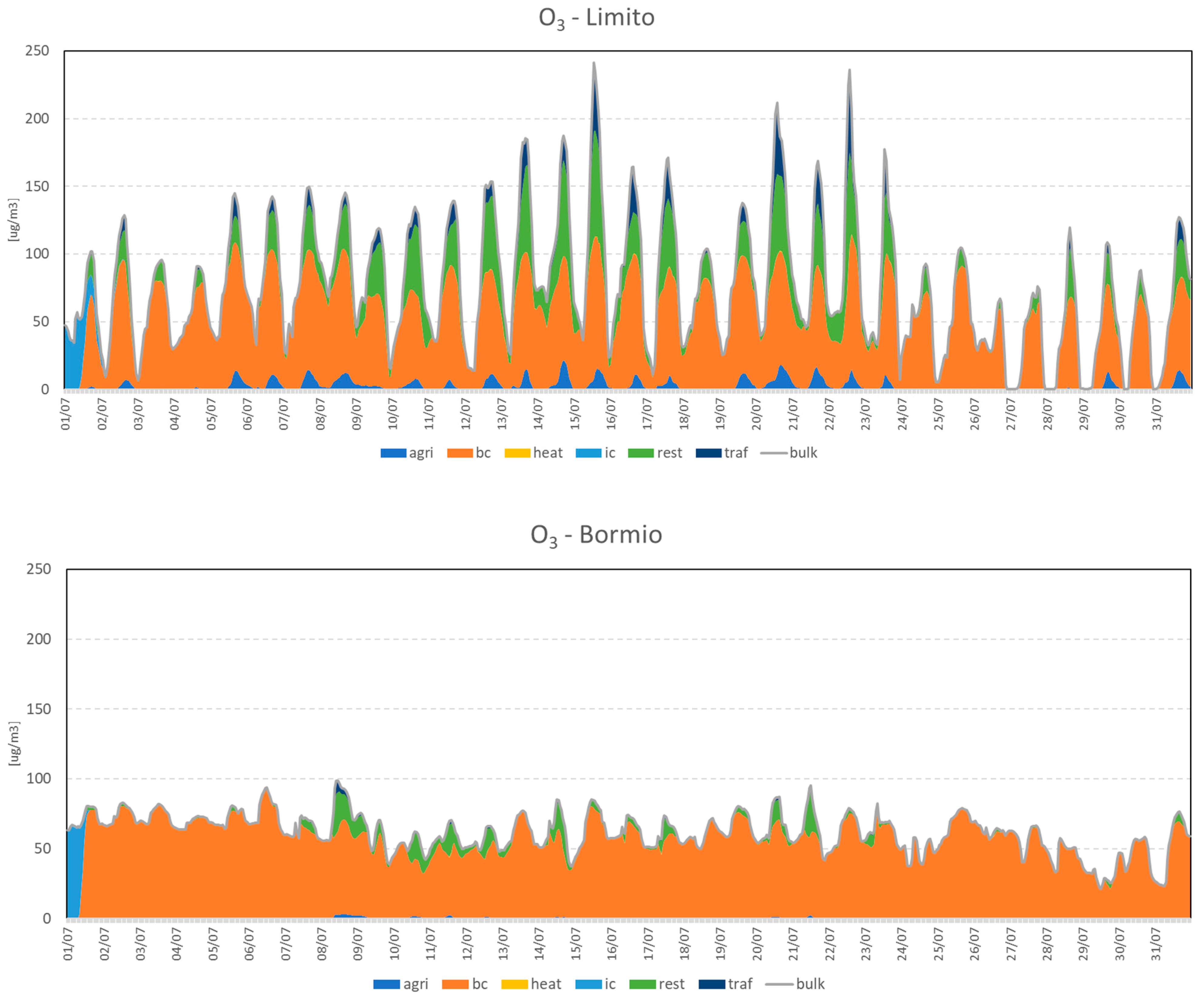
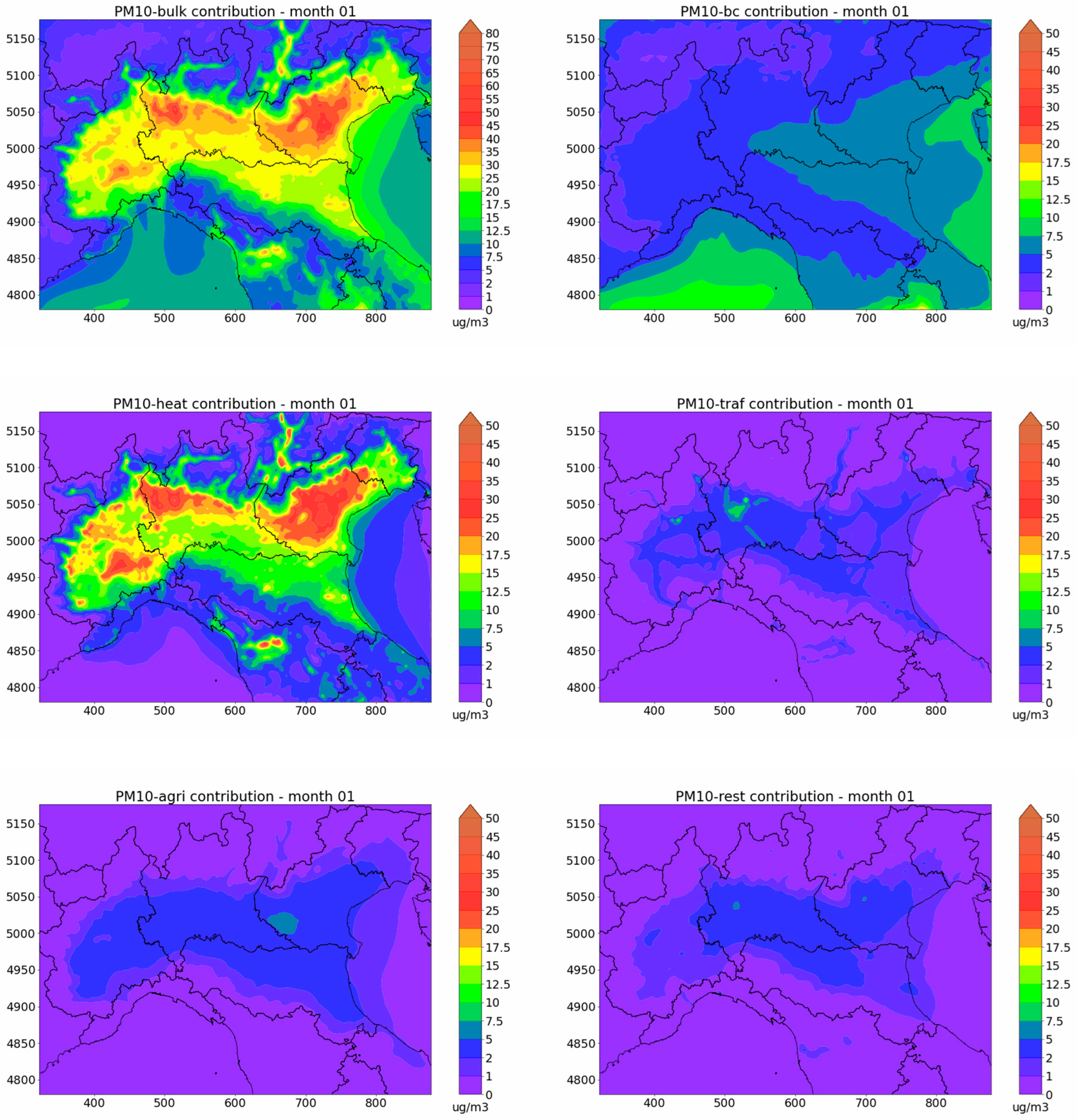
In this section, the contributions of SS are presented for the simulations over the three domains and shown as maps. To highlight sectorial contributions in a variety of geographical and emission conditions, three background stations were chosen: Limito, located in the Milan outskirts, monitoring background urban concentrations; Bormio, located at 1243 m of altitude, near a village in the floor of a long and sparsely populated Alpine valley; and Schivenoglia, monitoring a rural background in the middle of the highly urbanized Po Valley. The difference between Limito and Schivenoglia stations is mainly due to differences in urban emissions: the first one is affected by local and metropolitan emissions, even though it is not located in the city center, while the second one is far from large cities, being thus affected by rural emissions and the Po Valley background. Bormio is close to the LOMB domain border.

3.2.1. LOMB Domain

Figure 3 shows the absolute impact of the different sectors on PM10 monthly mean concentrations over the LOMB modelling domain.

The results are shown for January to better appreciate the contribution from residential heating. The map of bulk concentrations of PM10 (upper left) has a different scale with respect to the maps of absolute contributions from the sectors, allowing a better visualization of the spatial variability. Higher levels of PM10 are present in the center and southern area of Lombardy, where most human activities are localized. The contribution of the boundary conditions (upper right) to PM10 concentration shows a smooth pattern and tends to increase from North (Alpine region, minimum value 5 μg/m³) to South (plain area, maximum value about 20 μg/m³) due to the presence of relevant anthropogenic sources located southeast of the simulation domain, in the Po Valley. The spatial pattern of contribution from residential heating (center left map) clearly reflects the location of the populated areas and the fuels used: the highest concentrations are estimated at the foothills of the Alps, where more significant use of biomass, due to lower temperatures and lack of coverage of natural gas distribution networks, results in higher particulate emissions. In this area, biomass burning is estimated to be the most important contributor, leading to bulk concentrations exceeding 50 μg/m³. Local maxima are also visible over other major city centers, due to population density, while over rural areas in the Po Valley, concentration levels are between 7.5 and 12.5 μg/m³, mainly due to the advection from nearby areas and the formation of secondary components. The contribution of road traffic (center right map) is strictly related to traffic volumes, so the Milan conurbation is the hot spot of the Lombardy region, with contributions over the city center between 17.5 and 20 μg/m³. Significant contributions are also visible north of Milan and over the most important highways, with values between 7.5 and 12.5 μg/m³. Over rural and mountainous parts of the region, the contribution from the road traffic is generally low (under 5 μg/m³). Agriculture (bottom left map) plays a non-negligible role in PM10 formation, generating secondary components through chemical reactions in the atmosphere, reaching 7.5 μg/m³ in some areas.

The last group includes all remaining activities, not individually tagged (“rest”). Their contribution over the region is quite inhomogeneous, with local maxima (industrial sites) up to 10 μg/m³, and low values elsewhere.

Figure 4 shows the hourly evolution of contributions to PM10 concentrations in January at Limito, Bormio, and Schivenoglia.

At all sites, during the first day of simulation, the most important contribution is given by the IC. During the rest of the month, contributions from different sources vary according to local meteorology and emission levels. In Limito, the main contributors are heating and BC along the entire month, with road traffic and “rest” being relevant on some days, while agriculture is constantly low. Most hourly peaks are driven by rising contributions from heating combustion (e.g., on the 3rd, 7th, 16th, 18th, 22nd) and traffic (on the 3rd, 7th,19th, 29th). Despite its important role, the hourly trend of BC contribution is generally smoother during the month, with few exceptions (e.g., on the 15th). Total PM10 concentrations in Schivenoglia and Bormio are generally lower than in Limito, with less sharp hourly peaks. Residential heating is a local source that contributes to PM concentrations at all three sites. In Limito, on the outskirts of the Milan urban area, road traffic and industrial activities (included in “rest” SS) are also significant. Schivenoglia and Bormio are far from major urban and industrial areas, so the last two sectors do not show up significantly. Notwithstanding the distance between the three sites (almost 120 km) and the proximity to the domain border, BC contribution is almost the same in terms of magnitude and hourly variation, indicating an important secondary contribution from a broader area. The same effect is visible in the Bormio mountain location, where local sources’ impact is quite low and BC contribution is predominant over the whole period.

The comparison of hourly time series of contributions at different locations also allows us to highlight regional scale phenomena, for example, from the 09th to the 18th and from the 23rd to the 28th, when the BC contribution reaches values between 20 and 40 μg/m³, independently from the location. Lower BC contributions in Bormio are due to the particular location of the city: Alps at north and valley orientation constitute a barrier for pollution that comes from the Po Valley. This means that a massive PM10 contribution comes from sources located outside the calculation domain and possible actions on local sources would have a limited effect on total concentrations. This aspect is further discussed later.

Figure 5 shows the hourly evolution of contributions to O₃ concentrations at the same three sites during a summer month (July), when values are substantially higher than in winter.

At all sites, the IC contribution is present only during the first day of simulation, as in the case of PM10, while BC is the main individual contributor over the entire period of simulation, underlining the larger scale of O₃ formation, depending significantly also on sources located outside the calculation domain. In Limito, from the 6th to the 22nd, the second most important contribution is given by the “rest” set, which includes industrial activities and solvents use. Road traffic produces a lower contribution, that becomes larger only when concentrations exceed 100 µg/m³.

In the Bormio site, the SA changes significantly. Hourly values are constantly under 100 μg/m³, with less pronounced peaks, a contribution from “rest” significantly lower than in Limito, and a BC contribution responsible for almost all the calculated concentrations. These results are consistent with the fact that the site is very close to the boundary of the simulation domain, where the BC are more relevant, and the local anthropogenic emissions are quite low, the location being a small village in the Alps.

The Schivenoglia site presents a situation between Bormio and Limito, also due to its location within a rural context in the Po Valley. The SA shows ozone peaks less pronounced with respect to Limito, and BC as the main contributor, quite less than 100 μg/m³ over the whole period; the second most important contributor is the “rest” set of sources, including anthropogenic and natural sources.

Figure 6 shows at the same three locations the distribution of contributions to O₃ concentrations at 3 pm (taken as a proxy for the typical peak hour of concentrations during the day), averaged over July. As discussed for hourly time series, BC is the main contributor for O₃ concentrations, especially at Bormio, which is closer to the boundary and with an emission regime different from the Milan conurbation. At all locations, the “rest” set is the second most important contributor for O₃.

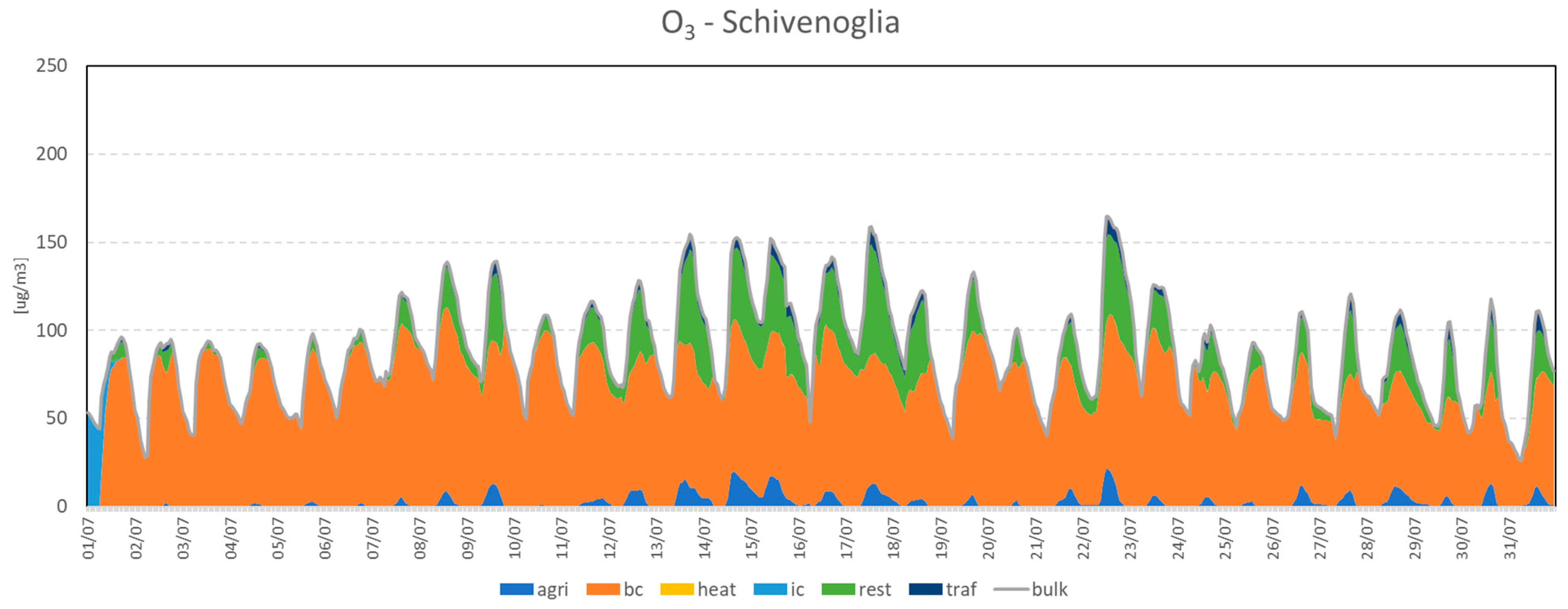
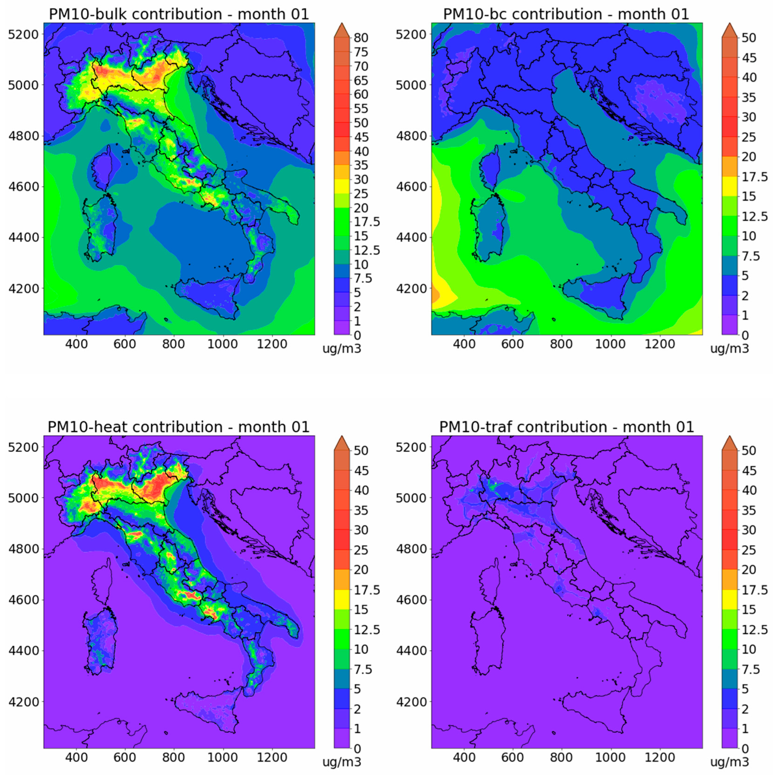
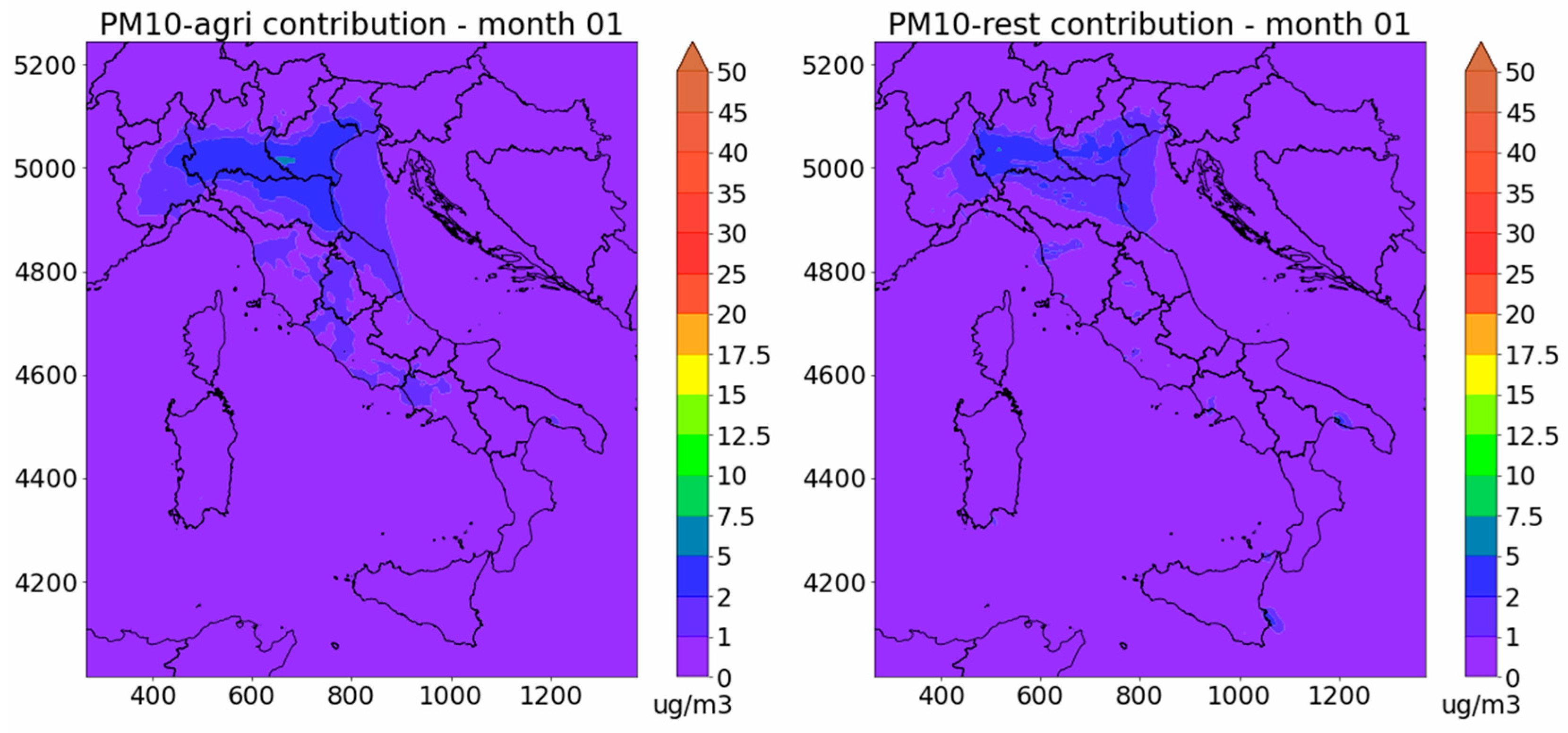
3.2.2. NI and IT Domains

Figure 7 illustrates the SA results for January monthly mean PM10 concentrations for the Northern Italy run. As in the LOMB run, high bulk concentrations (above 50 μg/m³, upper left map) are visible over the north of Milan, south area of Piedmont, and the large part of Veneto. Over the whole Po Valley, values are well above 20 μg/m³, with a clear regional background due to the homogeneity of meteorological conditions: low wind and mixing ratio, and similar temperatures and humidity, driving the atmospheric chemistry, leading to relevant production of secondary particulate matter.

Values of BC contributions (upper right) on Lombardy are remarkably lower with respect to the LOMB simulation, which is consistent with the fact that the distance of Lombardy from the boundaries of the domain NI is significantly longer than in the LOMB simulation. The contribution from heating (center left), as for spatial distribution and magnitude, is quite close to the LOMB simulation. The contribution from road traffic (center right) is lower in magnitude and similar in spatial pattern to LOMB, highlighting the Milan urban area and major highways. Agricultural (bottom left) and “rest” (bottom right) contributions are widely spread over the Po Valley, with an average effect of about 5 μg/m³.

Finally, Figure 8 shows the maps of contributions resulting from the IT simulation. The highest bulk concentrations (upper left) are visible over the Po Valley, the northern part of Tuscany, the southern part of Lazio, and Campania. Over Lombardy, with respect to the LOMB and NI simulations, the bulk PM10 behavior is similar, both in terms of magnitude and spatial pattern, while the BC contribution (upper right) is different: apart from Western Sardinia, where values reach 10 μg/m³, the contribution from sources outside the calculation domain on the mainland is lower than 5 μg/m³, consistent with a spatial domain larger than in LOMB and NI. In the overlapping parts, the contributions from heating, road traffic, agriculture, and “rest” are quite similar to what was estimated in NI simulations. Other hot spots appear in the center and the south of the country according to the spatial distribution of the sources previously discussed.

The comparisons of NI and IT with LOMB over their overlapping areas show that, despite the different model setups (dimension of the simulation domains, emission inventories, meteorological simulations, boundary conditions fields), similar maps of SS contributions (traffic, agriculture, heating, rest) are obtained, indicating that ORSA results are stable across domains with different sizes, if averaged over a sufficiently long period.

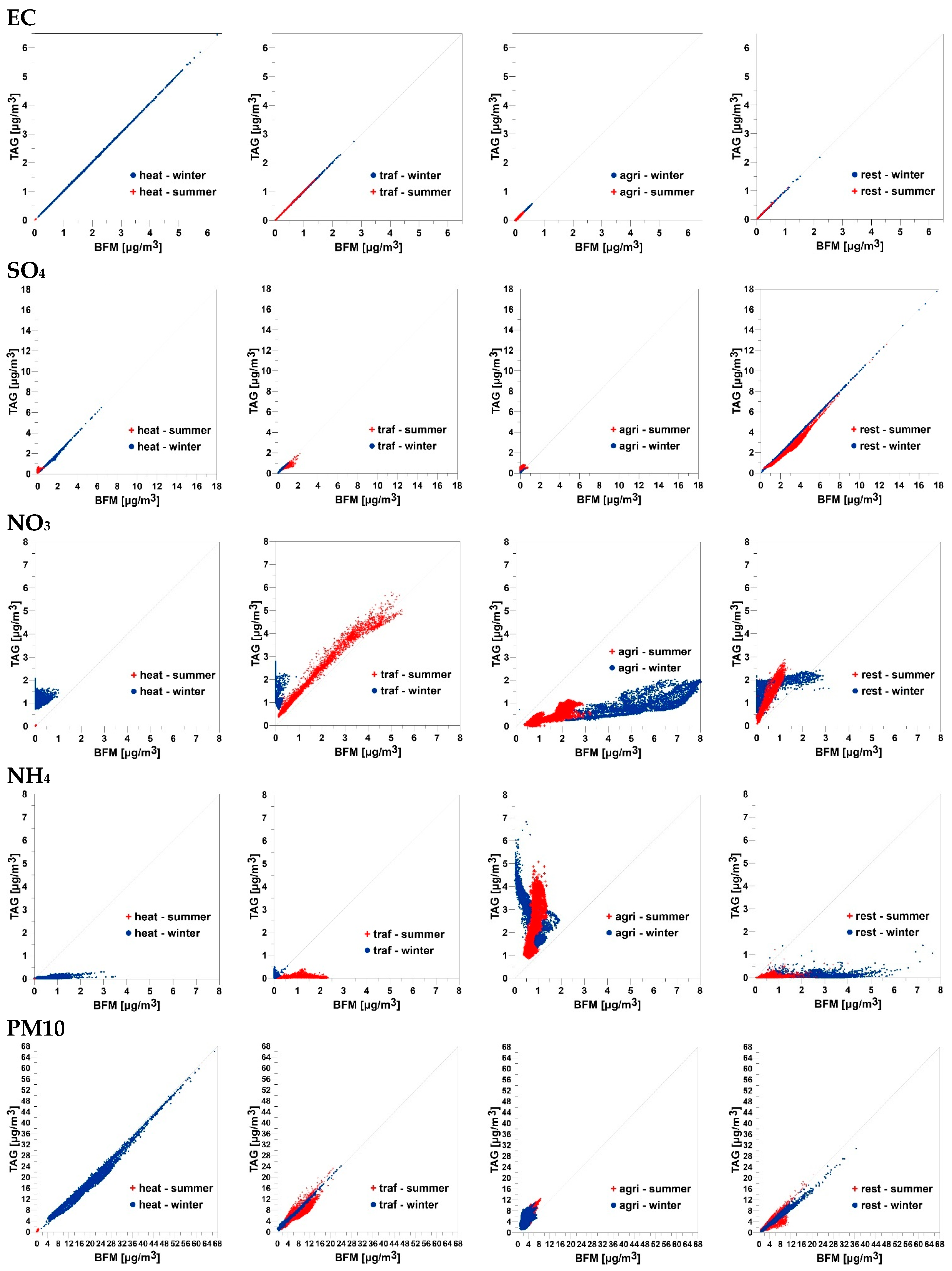
3.3. Comparison against Brute Force Method—LOMB

On the smallest domain, brute force method (BFM) calculations were also performed, considering the same source sets. This was realized through multiple sensitivity runs, one for each source set, where the emissions of all precursors of the implied sources were perturbed by −20% with respect to the base case values. Such perturbation magnitude, far from zero-out, was chosen to calculate model responses relatively close to the base case situation, as the tagged method inherently does, while avoiding numerical noise that may arise by considering smaller perturbations [56]. The impact of each source set was then estimated by considering the difference between the base case and the perturbed concentrations, normalized by the ratio between base case concentration values and the sum of the variations obtained for all source sets (heating, traffic, agriculture, rest). Differences with ORSA were expected, due to the presence of non-linearities in the responses that are not taken into account by the SA algorithm.

To make the ORSA contributions comparable in magnitude with BFM impacts, for each point of the domain, the contributions from the boundary conditions obtained with the tagged method were partitioned according to the distribution of the contributions to concentrations from the four sets of sources considered. This implicitly assumes that boundary conditions bring contributions from the sources outside the domain that are distributed in the same way as the contributions from the sources within the domain.

In Figure 9, the comparison between the two methods is reported in terms of scatter plots of average values computed for all points of the LOMB calculation grid for a winter and a summer month (January and July), to highlight the different behaviors depending on the presence of the various sources and the meteorological conditions affecting chemical transformations in the cold and hot period. As pointed out by [53], the greater the non-linearities in the relationships between precursor emissions and concentrations, the greater the differences expected between the results obtained with the two intrinsically different methods. This was in fact confirmed by the tests carried out.

Elemental carbon (EC) is not subject to chemical transformation, so the tagged and brute force methods give almost identical results, and effects due to the alteration of the aerosol dynamics, due to emission reduction in BFM, look negligible.

Results for sulfate (SO₄) show a strong correlation between the two methods, especially for the more relevant source-season combinations, i.e., heating in cold season and “rest” in both seasons, which notably include sources related to industrial activities and energy production.

For nitrate (NO₃) and ammonium (NH₄), results from the two methods are substantially different. As far as nitrate is concerned, the brute force approach attributes limited impacts to heating and traffic during the cold season, and substantial impacts to agriculture during both seasons. This almost has a counterpart in ammonium, with substantial impacts attributed to heating during the cold season and road traffic in summer, and limited impacts attributed to agriculture during both seasons. According to the tagged approach, heating and road traffic give otherwise significant contributions to cold season nitrate, while agriculture gives the dominant contribution to ammonium during both seasons, and a less pronounced contribution to nitrate. As pointed out by [4,5,53], these behaviors can depend on the way the two methods allocate the mass. The TAG method allocates the secondary components according to the mass of the precursors emitted; for example, the “agri” contribution at the NH₄NO₃ formation is evaluated by taking the (percentage) mass concentration ratio 100 * [NH₄]/([NH₄] + [NO₃]), where it is assumed the NH₄ contribution is almost completely allocated to “agri” (and similarly for sulphates). BFM otherwise allocates ammonia to other sources, evaluating the impact based on the amount of ammonium nitrate or ammonium sulphate which is not formed when “agri” sources are reduced.

The shape of distribution that can be seen in Figure 9, regarding the impact of “agri” on NH₄, is due to deviations from linearity in gas–aerosol thermodynamic equilibrium of NH₃/ammonium [56]. This also indirectly alters the dynamics of NO₃, the impact of “agri” on NO₃ being greater when calculated with BFM. This could perhaps also be due to the limited availability of NH₄, following NH₃ abatement, that leaves more HNO₃ in the atmosphere, which tends to be more effectively removed by dry deposition processes.

When PM10 is considered as a whole, the differences between the two methods are less dramatic, due to the compensation between the components that are overestimated or underestimated. It cannot be excluded that the chosen abatement percentage of −20% is not optimal for this comparison, because it amplifies the differences due to non-linearities, since it makes the system work where the deviations are more important.

This is consistent with [58], where a comprehensive discussion of these dynamics, in terms of sources’ contributions of the interaction terms, is given.

Although clearly evidencing for the different species the divergences between the two approaches, Figure 9 does not allow us to appreciate the spatial aspects. To address this, the maps of NH₄ and NO₃ contributions and impacts related to road traffic and agriculture, the source sectors on which tagged species and brute force methods disagree the most, are presented in Figures S4–S7 of the Supplementary Materials.

In the lower part of the domain, it is worth noting in January the relevance of agriculture contribution, as calculated by ORSA, on NO₃ over broad rural areas (Figure S2) and on NH₄ over urban areas (Figure S4). Urban areas are in general hot spots of emission of NO₂ (precursor of NO₃ and emitted mainly from traffic and heating), while agricultural areas are responsible for almost all emissions of NH₃ (precursor of NH₄ and emitted mainly from fertilizers and animal farming). In the applications shown here, during winter, the relevance of the contribution from agriculture on NO₃ in the agricultural plain (Figure S2), evidenced by BFM but not confirmed by ORSA, and on NH₄ in urban areas (Figure S4), conversely, evidenced by ORSA but not confirmed by BFM, demonstrates the different aspects involved in quantifying the role played by different sources in a complex atmospheric chemistry like the one of the Po Valley.

4. Discussion and Conclusions

This first application of the newly developed tagged species algorithm ORSA in the FARM chemical-transport model shows results of on-line source apportionment for PM10 and O₃ over multiple domains in Italy.

ORSA has been designed to be flexible enough and able to manage either sector or geographic contribution. This implementation provides a lean and fast tool (Fortran hybrid MPI-OpenMP) allowing us to avoid the burden of performing as many simulations as the number of sector/geographic contributions of interest. ORSA is available to Italian Environmental Regional Agencies for impact assessment.

In the present study, three simulations were performed at the same horizontal resolution over domains of increasing size, with the spatial extent ranging from the Lombardy region to Italy. To test the quality of “bulk” fields, a preliminary validation with measures available from the monitory network was conducted, finding an agreement comparable to other CTM validation studies. The impacts of agriculture, road traffic, domestic heating, and the rest of anthropogenic sources were estimated, together with contributions of boundary and initial conditions. Boundary conditions were treated as a sectorial source set but could also be interpreted as a geographical source set, being linked to sources outside the calculation domain. The use of different domain sizes allowed us to explore the spatial scale of the impact from BCs and the time relaxation scale related to the influence of initial conditions. Moreover, the use of different years for the simulations allowed us to test the sensitivity of source apportionment results to different but close periods.

The maps of the contributions from source sectors show an expected spatial inhomogeneity of contributions, as a consequence of the spatial variability of sectorial emissions and meteorological conditions. Over the overlapping areas, the contributions, computed through simulations performed at the same horizontal resolution over three domains of increasing size and over different but close periods, showed similar patterns. All simulations underline the consistency of the adopted apportionment algorithm.

The ORSA outputs were also compared to the brute force approach, by decreasing the emissions of each considered sources set by 20%. The two methods showed an exact linear matching regarding primary species, like EC, not involved in chemical reactions. Agriculture showed significant deviations from linearity, especially for what concerns ammonium and nitrates, depending on how the two methods evaluate the contributions: the TAG method allocates contributions according to the mass of the precursors emitted, while BFM measures the impact by evaluating the missing secondary PM caused by emissions abatement. Moreover, the contribution estimated by means of TAG is calculated in the context of the baseline complete emission set and the consequent atmospheric oxidation state. Substantial emission abatements on the other side may cause the system to work in different conditions, that is, different atmospheric oxidation state and aerosol regimes: free radicals and oxidated species obtain different values, as well as the diameter distributions of PM and even dry and wet deposition removal processes.

Finally, the resulting sectorial contributions are compared with the impacts computed via the brute force method, and the behavior of the two approaches is discussed.

This comparison confirmed what was found previously in the literature. TAG methods do not automatically lead to identifying sectorial priorities for emission reduction, or to a precise quantification of emission reductions needed to achieve concentration reductions. Emission reductions in fact modify the chemical composition of the atmosphere and may change the reaction pathways, leading even to an increase in pollution levels in some cases, and several studies (including the present) have identified substantial differences in applying source apportionment and sensitivity analysis in CTMs [58]. Therefore, in such cases, it is better to directly apply the full variations of interest to the emission input to models, to reflect the indirect effects caused by the potential change of atmospheric chemistry. However, the BFM approach also shows limitations, such as the high number of simulations (one for each emission reduction scenario) needed for evaluating real-life air quality plans acting on different sources. In fact, the existence of thresholds in the reduction of some emitted chemical species, beyond which non-linear effects on calculated concentrations may come into play, has been evidenced [6]. It is worth underlining that for some PM10 precursors, even for small perturbations, the results of BFM and TAG approaches may differ, due to the existence of interaction terms between source sectors. This happens because in TAG methods the interaction terms are split in fractions that are attributed to the contributions of sources, granting that the sum of their impacts corresponds to 100% of bulk atmospheric concentrations [58]. Therefore, the TAG approach can offer useful indications for orienting BFM studies. An important ongoing discussion is on how to compare and/or integrate source apportionment and sensitivity analyses, including in the Forum for Air quality Modelling (FAIRMODE), which recently gave specific recommendations on the topic, targeting the revision of the European Air Quality Directive [6].

Depending on pollutant and domain size, the time scale of the contribution from initial conditions spanned from one to two days for the smaller domain. The contribution from boundary conditions exhibited a clear dependence on domain size, with higher relative values on the smallest domain, then decreasing as the size of the domains increased. BCs provide a dominant contribution to ozone levels over all domains, while for PM10, their contribution is more relevant on the southernmost part of the IT and NI domains, which is mainly related to natural sources. The important role played by the domain dimension in BC contribution must be kept in mind when performing application studies and may be the subject of similar analyses using different apportionment algorithms.

Finally, the comparison performed between TAG and BFM gave further evidence that they respond to different purposes, and their combined use may provide a wide set of information useful for addressing the different air quality management needs.

References

1. European Commission, Joint Research Centre; Belis, C.A.; Favez, O.; Mircea, M.; Diapouli, E.; Manousakas, M.-I.; Vratolis, S.; Gilardoni, S.; Paglione, M.; Decesari, S.; et al. European Guide on Air Pollution Source Apportionment with Receptor Models: Revised Version 2019; Publications Office: Luxembourg, 2019. [Google Scholar]
2. Hopke, P.K. Review of Receptor Modeling Methods for Source Apportionment. J. Air Waste Manag. Assoc. 2016, 66, 237–259. [Google Scholar] [CrossRef] [PubMed]
3. Viana, M.; Kuhlbusch, T.A.J.; Querol, X.; Alastuey, A.; Harrison, R.M.; Hopke, P.K.; Winiwarter, W.; Vallius, M.; Szidat, S.; Prévôt, A.S.H.; et al. Source Apportionment of Particulate Matter in Europe: A Review of Methods and Results. J. Aerosol Sci. 2008, 39, 827–849. [Google Scholar] [CrossRef]
4. European Commission, Joint Research Centre; Belis, C.A.; Pirovano, G.; Mircea, M.; Calori, G. European Guide on Air Pollution Source Apportionment for Particulate Matter with Source Oriented Models and Their Combined Use with Receptor Models; Publications Office: Luxembourg, 2020. [Google Scholar]
5. Belis, C.A.; Pernigotti, D.; Pirovano, G.; Favez, O.; Jaffrezo, J.L.; Kuenen, J.; Denier van Der Gon, H.; Reizer, M.; Riffault, V.; Alleman, L.Y.; et al. Evaluation of Receptor and Chemical Transport Models for PM10 Source Apportionment. Atmos. Environ. X 2020, 5, 100053. [Google Scholar] [CrossRef]
6. European Commission, Joint Research Centre; Thunis, P.; Clappier, A.; Pirovano, G.; Riffault, V.; Gilardoni, S. Source Apportionment to Support Air Quality Management Practices: A Fitness for Purpose Guide (V 4.0); Publications Office: Luxembourg, 2022. [Google Scholar]
7. Thunis, P.; Clappier, A.; Tarrason, L.; Cuvelier, C.; Monteiro, A.; Pisoni, E.; Wesseling, J.; Belis, C.A.; Pirovano, G.; Janssen, S.; et al. Source Apportionment to Support Air Quality Planning: Strengths and Weaknesses of Existing Approaches. Environ. Int. 2019, 130, 104825. [Google Scholar] [CrossRef] [PubMed]
8. Burr, M.J.; Zhang, Y. Source Apportionment of Fine Particulate Matter over the Eastern U.S. Part I: Source Sensitivity Simulations Using CMAQ with the Brute Force Method. Atmos. Pollut. Res. 2011, 2, 300–317. [Google Scholar] [CrossRef]
9. Marmur, A.; Unal, A.; Mulholland, J.A.; Russell, A.G. Optimization-Based Source Apportionment of PM2.5 Incorporating Gas-to-Particle Ratios. Environ. Sci. Technol. 2005, 39, 3245–3254. [Google Scholar] [CrossRef] [PubMed]
10. EMEP. Transboundary Particulate Matter, Photo-Oxidants, Acidifying and Eutrophying Components; EMEP Satus Report 1/2015; EMEP: Ankara, Turkey, 2015. [Google Scholar]
11. Koo, B.; Wilson, G.M.; Morris, R.E.; Yarwood, G.; Dunker, A.M. Evaluation of CAMx Probing Tools for Particulate Matter; CRC Press: Boca Raton, FL, USA, 2009. [Google Scholar]
12. Thunis, P.; Degraeuwe, B.; Pisoni, E.; Trombetti, M.; Peduzzi, E.; Belis, C.A.; Wilson, J.; Clappier, A.; Vignati, E. PM2.5 Source Allocation in European Cities: A SHERPA Modelling Study. Atmos. Environ. 2018, 187, 93–106. [Google Scholar] [CrossRef]
13. Dunker, A.M. Efficient Calculation of Sensitivity Coefficients for Complex Atmospheric Models. Atmos. Environ. 1967, 15, 1155–1161. [Google Scholar] [CrossRef]
14. Dunker, A.M.; Yarwood, G.; Ortmann, J.P.; Wilson, G.M. The Decoupled Direct Method for Sensitivity Analysis in a Three-Dimensional Air Quality Model Implementation, Accuracy, and Efficiency. Environ. Sci. Technol. 2002, 36, 2965–2976. [Google Scholar] [CrossRef]
15. Koo, B.; Dunker, A.M.; Yarwood, G. Implementing the Decoupled Direct Method for Sensitivity Analysis in a Particulate Matter Air Quality Model. Environ. Sci. Technol. 2007, 41, 2847–2854. [Google Scholar] [CrossRef]
16. Napelenok, S.; Cohan, D.; Hu, Y.; Russell, A. Decoupled Direct 3D Sensitivity Analysis for Particulate Matter (DDM-3D/PM). Atmos. Environ. 2006, 40, 6112–6121. [Google Scholar] [CrossRef]
17. Yang, Y.-J.; Wilkinson, J.G.; Russell, A.G. Fast, Direct Sensitivity Analysis of Multidimensional Photochemical Models. Environ. Sci. Technol. 1997, 31, 2859–2868. [Google Scholar] [CrossRef]
18. Cohan, D.S.; Hakami, A.; Hu, Y.; Russell, A.G. Nonlinear Response of Ozone to Emissions: Source Apportionment and Sensitivity Analysis. Environ. Sci. Technol. 2005, 39, 6739–6748. [Google Scholar] [CrossRef] [PubMed]
19. Hakami, A.; Odman, M.T.; Russell, A.G. High-Order, Direct Sensitivity Analysis of Multidimensional Air Quality Models. Environ. Sci. Technol. 2003, 37, 2442–2452. [Google Scholar] [CrossRef] [PubMed]
20. Koo, B.; Yarwood, G.; Cohan, D.S. Higher-Order Decoupled Direct Method (HDDM) for Ozone Modeling Sensitivity Analyses and Code Refinements; ENVIRON International Corporation: Novato, CA, USA, 2008. [Google Scholar]
21. Zhang, W.; Capps, S.L.; Hu, Y.; Nenes, A.; Napelenok, S.L.; Russell, A.G. Development of the High-Order Decoupled Direct Method in Three Dimensions for Particulate Matter: Enabling Advanced Sensitivity Analysis in Air Quality Models. Geosci. Model Dev. 2012, 5, 355–368. [Google Scholar] [CrossRef]
22. Yarwood, G.; Morris, R.E.; Wilson, G.M. Particulate Matter Source Apportionment Technology (PSAT) in the CAMx Photochemical Grid Model. In Air Pollution Modeling and Its Application XVII; Borrego, C., Norman, A.-L., Eds.; Springer: Boston, MA, USA, 2007; pp. 478–492. [Google Scholar]
23. Yarwood, G.; Morris, R.; Yocke, M.; Hogo, H.; Chico, T. Development of a Methodology for Source Apportionment of Ozone Concentration Estimates from a Photochemical Grid Model; Air & Waste Management Association: Pittsburgh, PA, USA, 1996. [Google Scholar]
24. ENVIRON. CAMx—User’s Guide—Comprehensive Air Quality Model with Extensions—Version 6.1; Environ: Novato, CA, USA, 2014. [Google Scholar]
25. Wagstrom, K.M.; Pandis, S.N.; Yarwood, G.; Wilson, G.M.; Morris, R.E. Development and Application of a Computationally Efficient Particulate Matter Apportionment Algorithm in a Three-Dimensional Chemical Transport Model. Atmos. Environ. 2008, 42, 5650–5659. [Google Scholar] [CrossRef]
26. Bhave, P.V.; Pouliot, G.A.; Zheng, M. Diagnostic Model Evaluation for Carbonaceous PM2.5 Using Organic Markers Measured in the Southeastern U.S. Environ. Sci. Technol. 2007, 41, 1577–1583. [Google Scholar] [CrossRef]
27. Wang, Z.S.; Chien, C.-J.; Tonnesen, G.S. Development of a Tagged Species Source Apportionment Algorithm to Characterize Three-Dimensional Transport and Transformation of Precursors and Secondary Pollutants. J. Geophys. Res. 2009, 114, D21206. [Google Scholar] [CrossRef]
28. Kwok, R.H.F.; Napelenok, S.L.; Baker, K.R. Implementation and Evaluation of PM2.5 Source Contribution Analysis in a Photochemical Model. Atmos. Environ. 2013, 80, 398–407. [Google Scholar] [CrossRef]
29. Gao, J.; Zhu, B.; Xiao, H.; Kang, H.; Hou, X.; Shao, P. A Case Study of Surface Ozone Source Apportionment during a High Concentration Episode, under Frequent Shifting Wind Conditions over the Yangtze River Delta, China. Sci. Total Environ. 2016, 544, 853–863. [Google Scholar] [CrossRef]
30. Romero-Alvarez, J.; Lupaşcu, A.; Lowe, D.; Badia, A.; Acher-Nicholls, S.; Dorling, S.R.; Reeves, C.E.; Butler, T. Sources of Surface O3 in the UK: Tagging O3 within WRF-Chem; Gases/Atmospheric Modelling/Troposphere/Chemistry (chemical composition and reactions); EGU: Munich, Germany, 2022. [Google Scholar]
31. Zhao, Y.; Li, Y.; Kumar, A.; Ying, Q.; Vandenberghe, F.; Kleeman, M.J. Separately Resolving NOx and VOC Contributions to Ozone Formation. Atmos. Environ. 2022, 285, 119224. [Google Scholar] [CrossRef]
32. Brandt, J.; Silver, J.D.; Christensen, J.H.; Andersen, M.S.; Bønløkke, J.H.; Sigsgaard, T.; Geels, C.; Gross, A.; Hansen, A.B.; Hansen, K.M.; et al. Contribution from the Ten Major Emission Sectors in Europe and Denmark to the Health-Cost Externalities of Air Pollution Using the EVA Model System—An Integrated Modelling Approach. Atmos. Chem. Phys. 2013, 13, 7725–7746. [Google Scholar] [CrossRef]
33. Kranenburg, R.; Segers, A.J.; Hendriks, C.; Schaap, M. Source Apportionment Using LOTOS-EUROS: Module Description and Evaluation. Geosci. Model Dev. 2013, 6, 721–733. [Google Scholar] [CrossRef]
34. Pay, M.T.; Gangoiti, G.; Guevara, M.; Napelenok, S.; Querol, X.; Jorba, O.; Pérez García-Pando, C. Ozone Source Apportionment during Peak Summer Events Over Southwestern Europe. Atmos. Chem. Phys. 2019, 19, 5467–5494. [Google Scholar] [CrossRef] [PubMed]
35. Pepe, N.; Pirovano, G.; Balzarini, A.; Toppetti, A.; Riva, G.M.; Amato, F.; Lonati, G. Enhanced CAMx Source Apportionment Analysis at an Urban Receptor in Milan Based on Source Categories and Emission Regions. Atmos. Environ. X 2019, 2, 100020. [Google Scholar] [CrossRef]
36. Lupaşcu, A.; Butler, T. Source Attribution of European Surface O3 Using a Tagged O3 Mechanism. Atmos. Chem. Phys. 2019, 19, 14535–14558. [Google Scholar] [CrossRef]
37. ARIANET. FARM (Flexible Air Quality Regional Model)—Model Formulation and User Manual—Version 5.1; ARIANET S.R.L.: Milan, Italy, 2020. [Google Scholar]
38. Silibello, C.; Calori, G.; Brusasca, G.; Giudici, A.; Angelino, E.; Fossati, G.; Peroni, E.; Buganza, E. Modelling of PM10 Concentrations over Milano Urban Area Using Two Aerosol Modules. Environ. Model. Softw. 2008, 23, 333–343. [Google Scholar] [CrossRef]
39. D’Elia, I.; Briganti, G.; Vitali, L.; Piersanti, A.; Righini, G.; D’Isidoro, M.; Cappelletti, A.; Mircea, M.; Adani, M.; Zanini, G.; et al. Measured and Modelled Air Quality Trends in Italy over the Period 2003–2010. Atmos. Chem. Phys. 2021, 21, 10825–10849. [Google Scholar] [CrossRef]
40. Mircea, M.; Ciancarella, L.; Briganti, G.; Calori, G.; Cappelletti, A.; Cionni, I.; Costa, M.; Cremona, G.; D’Isidoro, M.; Finardi, S.; et al. Assessment of the AMS-MINNI System Capabilities to Simulate Air Quality over Italy for the Calendar Year 2005. Atmos. Environ. 2014, 84, 178–188. [Google Scholar] [CrossRef]
41. Adani, M.; Piersanti, A.; Ciancarella, L.; D’Isidoro, M.; Villani, M.G.; Vitali, L. Preliminary Tests on the Sensitivity of the FORAIR_IT Air Quality Forecasting System to Different Meteorological Drivers. Atmosphere 2020, 11, 574. [Google Scholar] [CrossRef]
42. Adani, M.; D’Isidoro, M.; Mircea, M.; Guarnieri, G.; Vitali, L.; D’Elia, I.; Ciancarella, L.; Gualtieri, M.; Briganti, G.; Cappelletti, A.; et al. Evaluation of Air Quality Forecasting System FORAIR-IT over Europe and Italy at High Resolution for Year 2017. Atmos. Pollut. Res. 2022, 13, 101456. [Google Scholar] [CrossRef]
43. SNPA. Descrizione dei Modelli di Qualità Dell’aria Utilizzati Nell’ambito del Sistema Agenziale e Delle Relative Caratteristiche Tecniche e di Disponibilità; ISPRA (Italian Institute for Environmental Protection and Research): Lombardy, Italy; National Network for the Environmental Protection (SNPA): Santa Monica, CA, USA, 2016. [Google Scholar]
44. Sandu, A.; Daescu, D.N.; Carmichael, G.R. Direct and Adjoint Sensitivity Analysis of Chemical Kinetic Systems with KPP: Part I—Theory and Software Tools. Atmos. Environ. 2003, 37, 5083–5096. [Google Scholar] [CrossRef]
45. Carter, W.P.L. Documentation of the SAPRC-99 Chemical Mechanism for VOC Reactivity Assessment; University of California: Riverside, CA, USA, 2000. [Google Scholar]
46. Binkowski, F.S.; Roselle, S.J. Models-3 Community Multiscale Air Quality (CMAQ) Model Aerosol Component 1. Model Description. J. Geophys. Res. 2003, 108, 2001JD001409. [Google Scholar] [CrossRef]
47. Fountoukis, C.; Nenes, A. ISORROPIA II: A Computationally Efficient Aerosol Thermodynamic Equilibrium Model for K+, Ca2+, Mg2+, NH4+, Na+, SO42−, NO3−, Cl, H2O Aerosols. Atmos. Chem. Phys. 2007, 7, 4639–4659. [Google Scholar] [CrossRef]
48. Schell, B.; Ackermann, I.J.; Hass, H.; Binkowski, F.S.; Ebel, A. Modeling the Formation of Secondary Organic Aerosol within a Comprehensive Air Quality Model System. J. Geophys. Res. 2001, 106, 28275–28293. [Google Scholar] [CrossRef]
49. EEA. Air Quality in Europe 2021; European Environment Agency Report No. 15/2021; European Environment Agency: Copenhagen, Denmark, 2021.
50. Piersanti, A.; D’Elia, I.; Gualtieri, M.; Briganti, G.; Cappelletti, A.; Zanini, G.; Ciancarella, L. The Italian National Air Pollution Control Programme: Air Quality, Health Impact and Cost Assessment. Atmosphere 2021, 12, 196. [Google Scholar] [CrossRef]
51. Jakovljević, T.; Lovreškov, L.; Jelić, G.; Anav, A.; Popa, I.; Fornasier, M.F.; Proietti, C.; Limić, I.; Butorac, L.; Vitale, M.; et al. Impact of Ground-Level Ozone on Mediterranean Forest Ecosystems Health. Sci. Total Environ. 2021, 783, 147063. [Google Scholar] [CrossRef] [PubMed]
52. Michetti, M.; Gualtieri, M.; Anav, A.; Adani, M.; Benassi, B.; Dalmastri, C.; D’Elia, I.; Piersanti, A.; Sannino, G.; Zanini, G.; et al. Climate Change and Air Pollution: Translating Their Interplay into Present and Future Mortality Risk for Rome and Milan Municipalities. Sci. Total Environ. 2022, 830, 154680. [Google Scholar] [CrossRef] [PubMed]
53. Belis, C.A.; Pirovano, G.; Villani, M.G.; Calori, G.; Pepe, N.; Putaud, J.P. Comparison of Source Apportionment Approaches and Analysis of Non-Linearity in a Real Case Model Application. Geosci. Model Dev. 2021, 14, 4731–4750. [Google Scholar] [CrossRef]
54. Arunachalam, S. Peer Review of Source Apportionment Tools in CAMx and CMAQ; University of North Carolina Institute for the Environment: Chapel Hill, NC, USA, 2009. [Google Scholar]
55. Burr, M.J.; Zhang, Y. Source Apportionment of Fine Particulate Matter over the Eastern U.S. Part II: Source Apportionment Simulations Using CAMx/PSAT and Comparisons with CMAQ Source Sensitivity Simulations. Atmos. Pollut. Res. 2011, 2, 318–336. [Google Scholar] [CrossRef]
56. Koo, B.; Wilson, G.M.; Morris, R.E.; Dunker, A.M.; Yarwood, G. Comparison of Source Apportionment and Sensitivity Analysis in a Particulate Matter Air Quality Model. Environ. Sci. Technol. 2009, 43, 6669–6675. [Google Scholar] [CrossRef] [PubMed]
57. Butler, T.; Lupascu, A.; Nalam, A. Attribution of Ground-Level Ozone to Anthropogenic and Natural Sources of Nitrogen Oxides and Reactive Carbon in a Global Chemical Transport Model. Atmos. Chem. Phys. 2020, 20, 10707–10731. [Google Scholar] [CrossRef]
58. Clappier, A.; Belis, C.A.; Pernigotti, D.; Thunis, P. Source Apportionment and Sensitivity Analysis: Two Methodologies with Two Different Purposes. Geosci. Model Dev. 2017, 10, 4245–4256. [Google Scholar] [CrossRef]
59. Grewe, V.; Tsati, E.; Hoor, P. On the Attribution of Contributions of Atmospheric Trace Gases to Emissions in Atmospheric Model Applications. Geosci. Model Dev. 2010, 3, 487–499. [Google Scholar] [CrossRef]
60. Kwok, R.H.F.; Baker, K.R.; Napelenok, S.L.; Tonnesen, G.S. Photochemical Grid Model Implementation and Application of VOC, NOx, and O3 Source Apportionment. Geosci. Model Dev. 2015, 8, 99–114. [Google Scholar] [CrossRef]
61. Kumar, N.; Lurmann, F.W. Peer Review of ENVIRON’s Ozone Source Apportionment Technology and CAMx Air Quality Model; Sonoma Technology, Inc.: Santa Rosa, CA, USA, 1997. [Google Scholar]
62. Sillman, S. The Use of NOy, H2O2, and HNO3 as Indicators for Ozone-NOx-Hydrocarbon Sensitivity in Urban Locations. J. Geophys. Res. 1995, 100, 14175. [Google Scholar] [CrossRef]
63. Seinfeld, J.H.; Pandis, S.N. Atmospheric Chemistry and Physics from Air Pollution to Climate Change; Wiley-Interscience—John Wiley & Sons: New York, NY, USA, 1998; ISBN 978-0-471-17816-3. [Google Scholar]
64. ARPA. Lombardia. INEMAR—Inventario Emissioni Aria—ARPA Regione Lombardia; ARPA: Lombardy, Italy, 2014. [Google Scholar]
65. ISPRA. Italian Emission Inventory 1990–2019. Informative Inventory Report 2021; ISPRA: Rome, Italy, 2021. [Google Scholar]
66. Kuenen, J.J.P.; Visschedijk, A.J.H.; Jozwicka, M.; Denier van der Gon, H.A.C. TNO-MACC_II Emission Inventory; a Multi-Year (2003–2009) Consistent High-Resolution European Emission Inventory for Air Quality Modelling. Atmos. Chem. Phys. 2014, 14, 10963–10976. [Google Scholar] [CrossRef]
67. ARIA Technologies. ARIANET Emission Manager—Processing System for Model-Ready Emission Input—User’s Guide; ARIA Technologies: Paris, France, 2013. [Google Scholar]
68. Guenther, A.; Karl, T.; Harley, P.; Wiedinmyer, C.; Palmer, P.I.; Geron, C. Estimates of Global Terrestrial Isoprene Emissions Using MEGAN (Model of Emissions of Gases and Aerosols from Nature). Atmos. Chem. Phys. 2006, 6, 3181–3210. [Google Scholar] [CrossRef]
69. EEA. EMEP/CORINAIR Atmospheric Emission Inventory Guidebook—Second Edition 1999. European Environment Agency; Technical Report No 30/2000; EEA: Copenhagen, Denmark, 2000. [Google Scholar]
70. Veratti, G.; Stortini, M.; Amorati, R.; Bressan, L.; Giovannini, G.; Bande, S.; Bissardella, F.; Ghigo, S.; Angelino, E.; Colombo, L.; et al. Impact of NOx and NH3 Emission Reduction on Particulate Matter across Po Valley: A LIFE-IP-PREPAIR Study. Atmosphere 2023, 14, 762. [Google Scholar] [CrossRef]
71. D’Isidoro, M.; D’Elia, I.; Vitali, L.; Briganti, G.; Cappelletti, A.; Piersanti, A.; Finardi, S.; Calori, G.; Pepe, N.; Di Giosa, A.; et al. Lessons Learnt for Air Pollution Mitigation Policies from the COVID-19 Pandemic: The Italian Perspective. Atmos. Pollut. Res. 2022, 13, 101620. [Google Scholar] [CrossRef]
72. D’Allura, A.; Costa, M.P.; Silibello, C. QualeAria: European and National Scale Air Quality Forecast System Performance Evaluation. IJEP 2018, 64, 110. [Google Scholar] [CrossRef]
73. Pielke, R.A.; Cotton, W.R.; Walko, R.L.; Tremback, C.J.; Lyons, W.A.; Grasso, L.D.; Nicholls, M.E.; Moran, M.D.; Wesley, D.A.; Lee, T.J.; et al. A Comprehensive Meteorological Modeling System—RAMS. Meteorl. Atmos. Phys. 1992, 49, 69–91. [Google Scholar] [CrossRef]
74. ARIA. Technologies SWIFT Wind Field Model, General Design Manual; ARIA Technologies: Paris, France, 2010. [Google Scholar]
75. Heymann, Y. (Ed.) CORINE Land Cover: Technical Guide; Office for Official Publications of the European Communities: Luxembourg, 1994; ISBN 978-92-826-2578-1. [Google Scholar]
76. Vitali, L.; Adani, M.; Ciancarella, L.; Cremona, G.; D’Isidoro, M.; Mircea, M.; Piersanti, A.; Briganti, G.; Cappelletti, A.; D’Elia, I.; et al. AMS-MINNI National Air Quality Simulation on Italy for the Calendar Year 2015. Annual Air Quality Simulation of MINNI Atmospheric Modelling System: Results for the Calendar Year 2015 and Comparison with Observed Data; ENEA Technical Report, RT/2019/15/ENEA; ENEA: Stockholm, Sweden, 2019. [Google Scholar]
77. Inness, A.; Ades, M.; Agustí-Panareda, A.; Barré, J.; Benedictow, A.; Blechschmidt, A.-M.; Dominguez, J.J.; Engelen, R.; Eskes, H.; Flemming, J.; et al. The CAMS Reanalysis of Atmospheric Composition. Atmos. Chem. Phys. 2019, 19, 3515–3556. [Google Scholar] [CrossRef]
78. Skamarock, W.C.; Klemp, J.B.; Dudhia, J.; Gill, D.O.; Liu, Z.; Berner, J.; Wang, W.; Powers, J.G.; Duda, M.G.; Barker, D.M.; et al. A Description of the Advanced Research WRF Model Version 4; National Center for Atmospheric Research: Boulder, CO, USA, 2008. [Google Scholar]
79. Marras, G.F.; Silibello, C.; Calori, G. A Hybrid Parallelization of Air Quality Model with MPI and OpenMP. In Recent Advances in the Message Passing Interface; Träff, J.L., Benkner, S., Dongarra, J.J., Eds.; Lecture Notes in Computer Science; Springer: Berlin/Heidelberg, Germany, 2012; Volume 7490, pp. 235–245. ISBN 978-3-642-33517-4. [Google Scholar]
80. Iannone, F.; Ambrosino, F.; Bracco, G.; De Rosa, M.; Funel, A.; Guarnieri, G.; Migliori, S.; Palombi, F.; Ponti, G.; Santomauro, G.; et al. CRESCO ENEA HPC Clusters: A Working Example of a Multifabric GPFS Spectrum Scale Layout. In Proceedings of the 2019 International Conference on High Performance Computing & Simulation (HPCS), Dublin, Ireland, 15–19 July 2019; IEEE: Dublin, Ireland, 2019; pp. 1051–1052. [Google Scholar]
81. Chang, J.C.; Hanna, S.R. Air Quality Model Performance Evaluation. Meteorol. Atmos. Phys. 2004, 87, 167–196. [Google Scholar] [CrossRef]
82. Bessagnet, B.; Pirovano, G.; Mircea, M.; Cuvelier, C.; Aulinger, A.; Calori, G.; Ciarelli, G.; Manders, A.; Stern, R.; Tsyro, S.; et al. Presentation of the EURODELTA III Intercomparison Exercise—Evaluation of the Chemistry Transport Models’ Performance on Criteria Pollutants and Jointanalysis with Meteorology. Atmos. Chem. Phys. 2016, 16, 12667–12701. [Google Scholar] [CrossRef]
83. Schaap, M.; Cuvelier, C.; Hendriks, C.; Bessagnet, B.; Baldasano, J.M.; Colette, A.; Thunis, P.; Karam, D.; Fagerli, H.; Graff, A.; et al. Performance of European Chemistry Transport Models as Function of Horizontal Resolution. Atmos. Environ. 2015, 112, 90–105. [Google Scholar] [CrossRef]
Scheme 1. The dominating regime depends on the indicator value as in the following scheme.
Atmosphere 15 00191 sch001
Figure 1. Maps showing the three domains (IT, NI, LOMB) and the three stations of Lombardy that are considered in the discussion on sector contribution.
Atmosphere 15 00191 g001
Figure 2. Total anthropogenic emissions of main pollutants over Lombardy and sectorial share, according to the two inventories employed: regional (LOMB) for the year 2012 and national (NI, IT) for the year 2015.
Atmosphere 15 00191 g002
Figure 3. LOMB domain. Bulk concentrations (upper left) and absolute contributions to PM10 monthly mean concentrations in January, from boundary conditions (upper right) and the considered source sets (middle and lower maps).
Atmosphere 15 00191 g003
Figure 4. Hourly evolution of contributions to PM10 concentrations at Limito, Bormio, and Schivenoglia, in January.
Atmosphere 15 00191 g004aAtmosphere 15 00191 g004b
Figure 5. Hourly evolution of contributions to O3 concentrations at Limito and Bormio, in July.
Atmosphere 15 00191 g005aAtmosphere 15 00191 g005b
Figure 6. Distribution of the average contributions to O3 concentrations at 3 pm for the month of July.
Atmosphere 15 00191 g006
Figure 7. NI domain. Bulk concentrations (upper left) and absolute contributions to PM10 monthly mean concentrations in January, from boundary conditions (upper right) and the considered source sets (middle and lower maps).
Atmosphere 15 00191 g007
Figure 8. IT domain. Bulk concentrations (upper left) and absolute contributions to PM10 monthly mean concentrations in January, from boundary conditions (upper right) and the considered source sets (middle and lower maps).
Atmosphere 15 00191 g008aAtmosphere 15 00191 g008b
Figure 9. Monthly mean concentrations in January and July: comparison between brute force impacts and tagged species contributions for PM10 components and total PM10, by emission source.
Atmosphere 15 00191 g009