
Reconstructed Phase Space of Tropical Cyclone Activity in the North Atlantic Basin for Determining the Predictability of the System

 ,
, 
Abstract
1. Introduction
2. Data and Methods
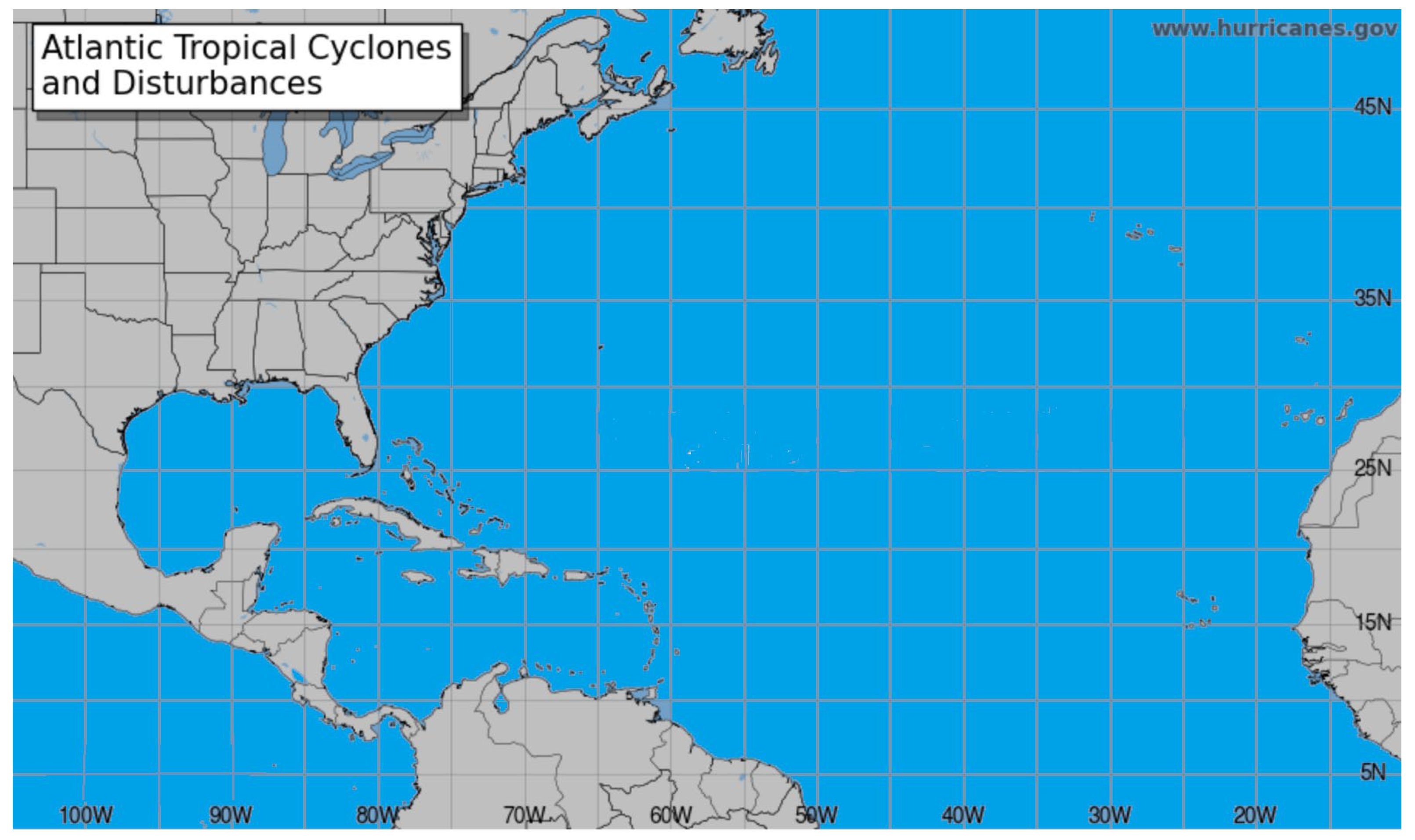
2.1. Study Region
2.2. Data
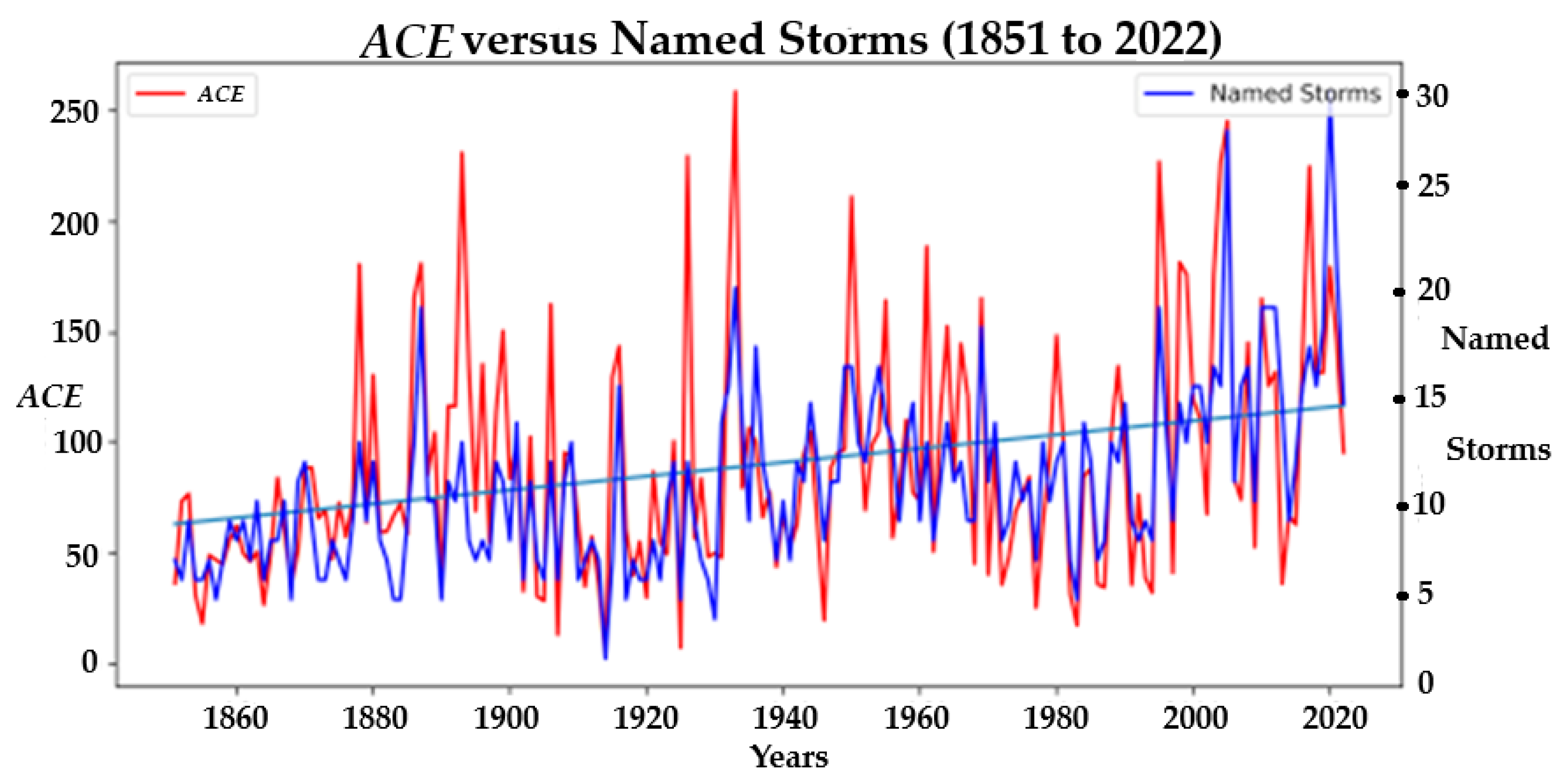
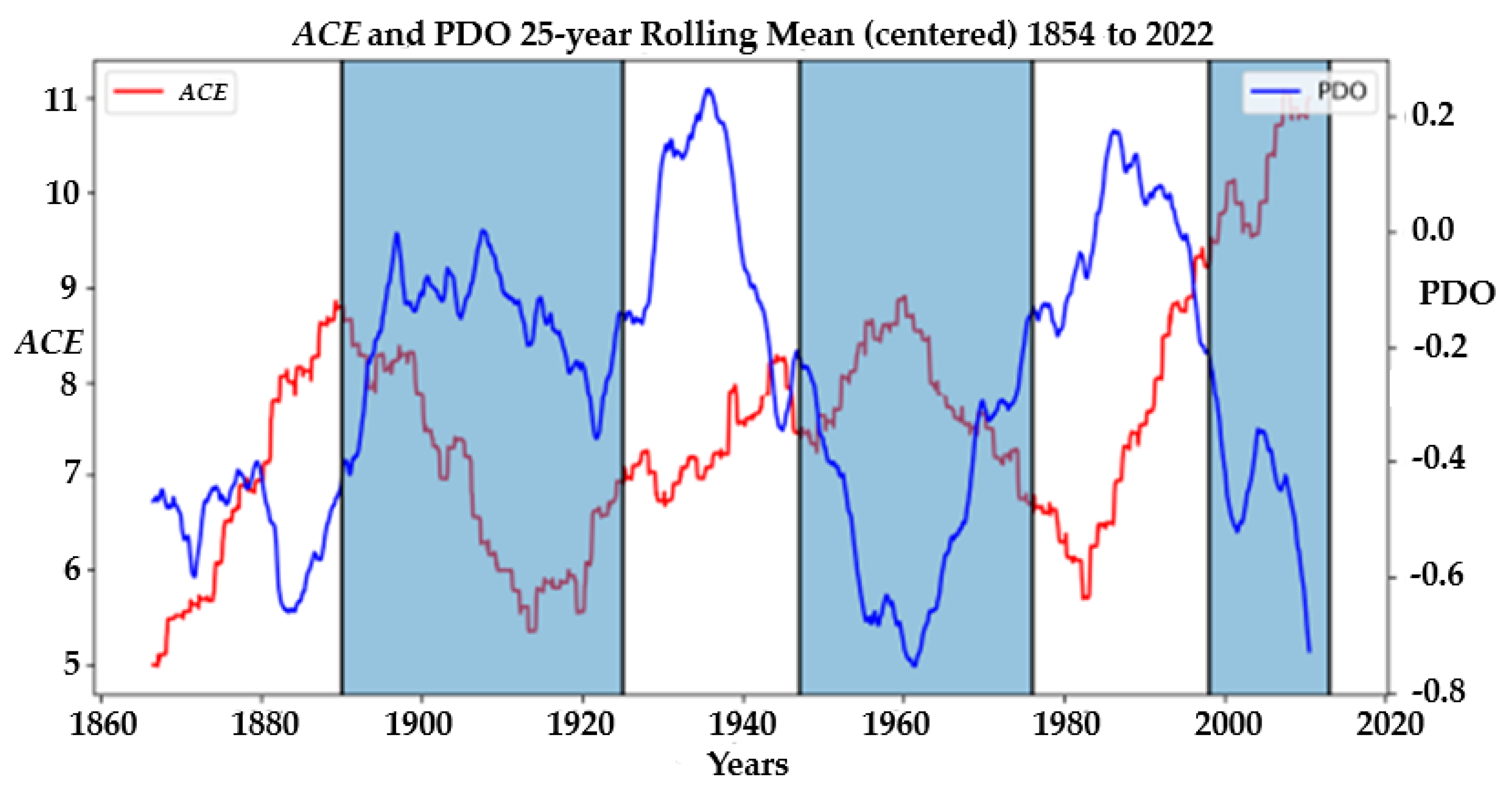
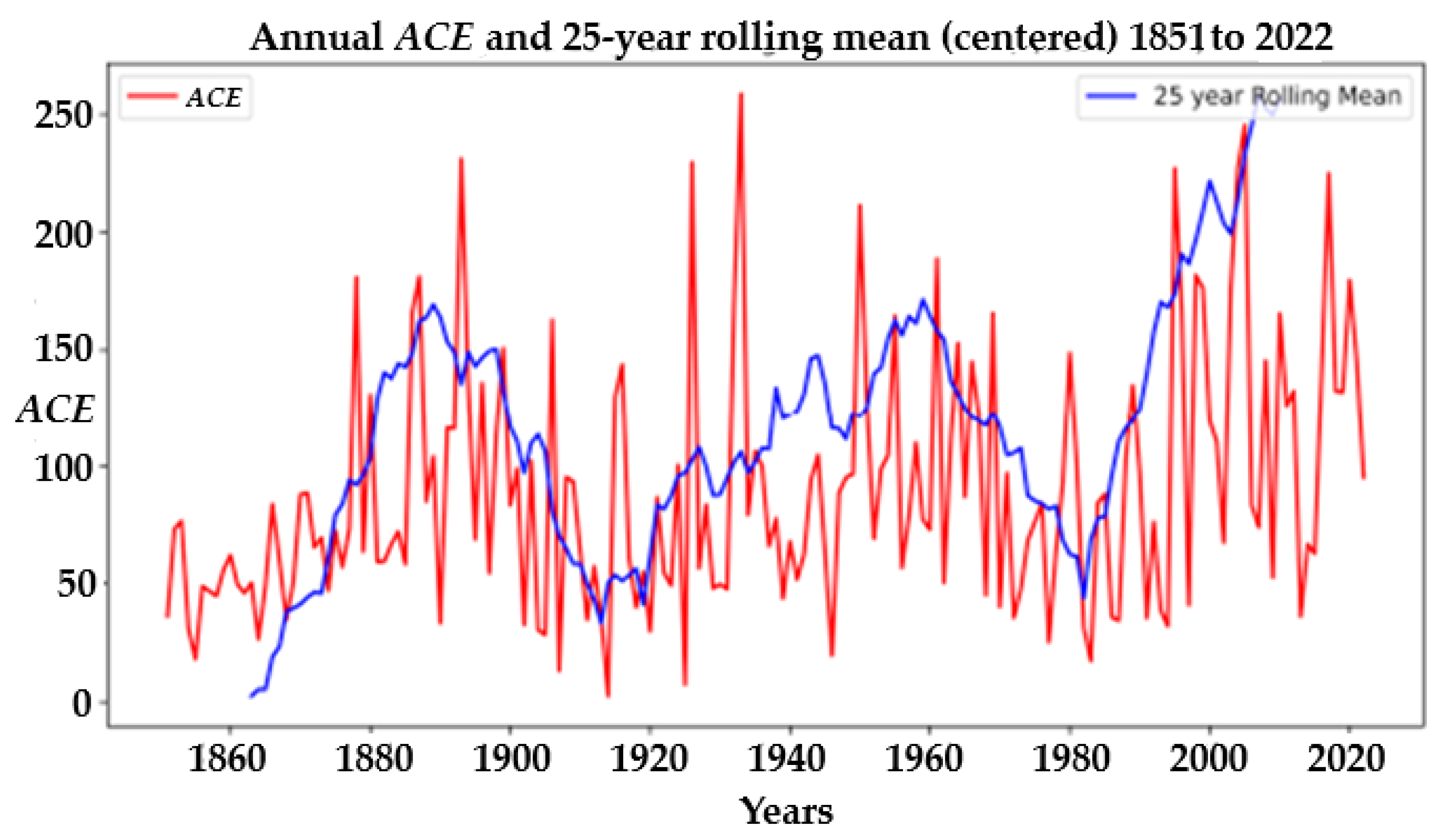
2.3. Time Series
3. Results
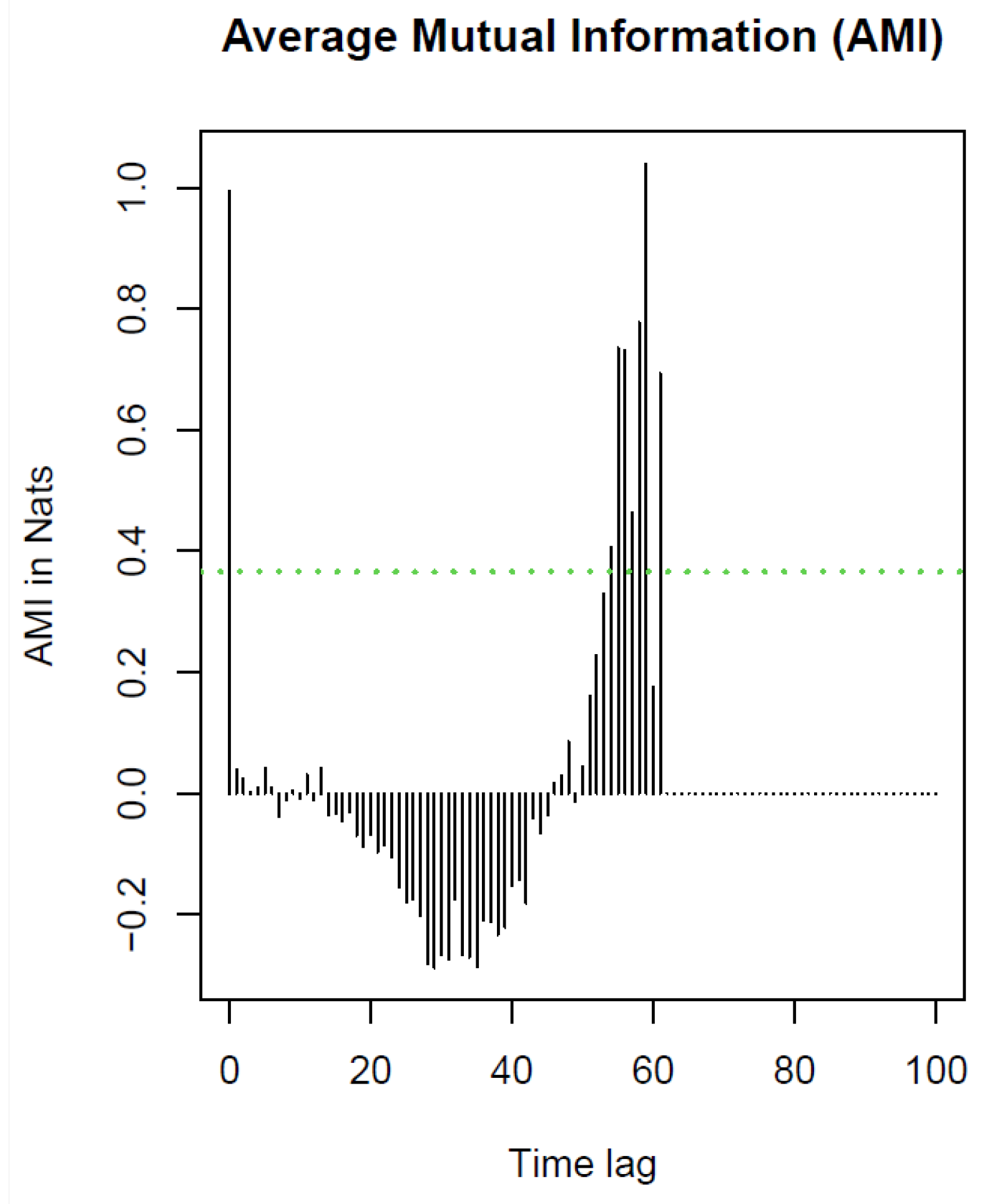
3.1. Time Delay with Auto Mutual Information (AMI)
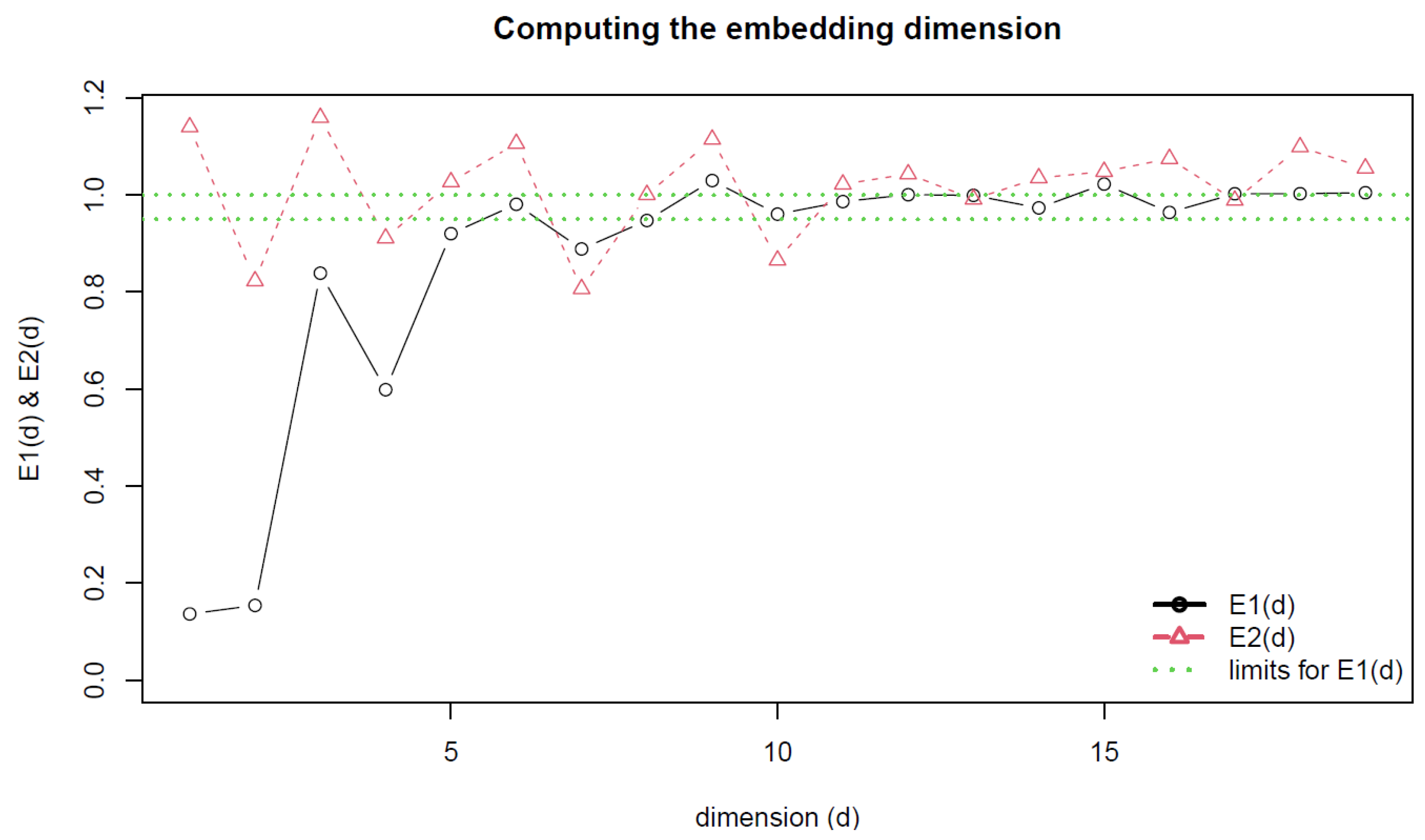
3.2. Embedded Dimensions Based on Cao’s Algorithm
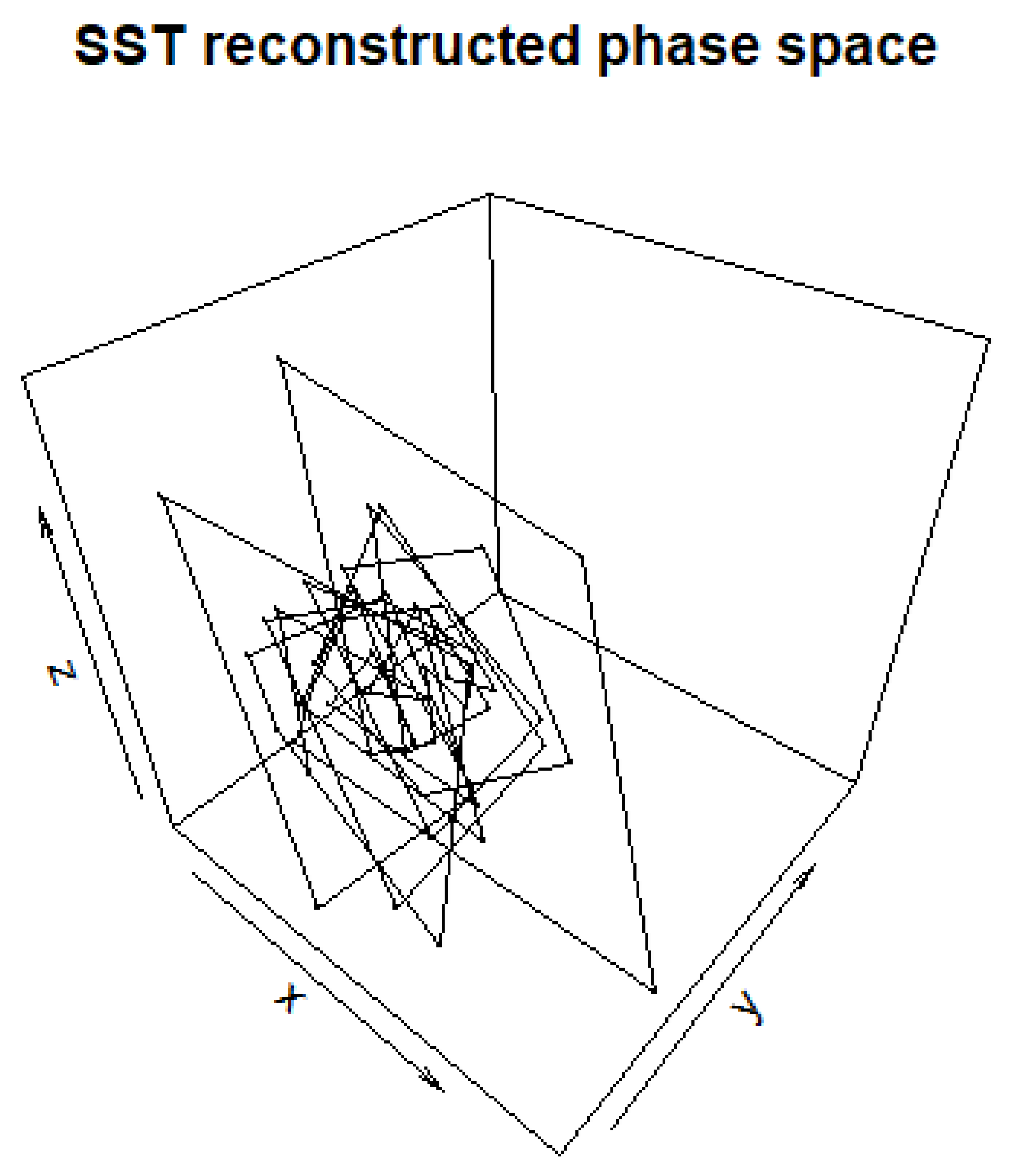
3.3. Takens’ Theorem
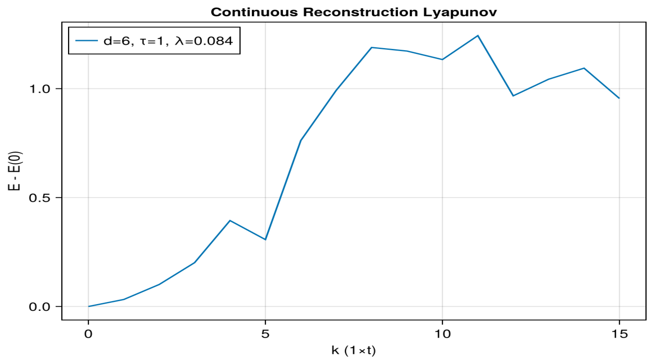
3.4. Lyapunov Exponent
4. Discussion
5. Conclusions
Author Contributions
Funding
Institutional Review Board Statement
Informed Consent Statement
Data Availability Statement
Acknowledgments
Conflicts of Interest
Abbreviations
| ACE | Accumulated Cyclone Energy |
| NHC | National Hurricane Center |
| ENSO | El Niño Southern Oscillation |
| PDO | Pacific Decadal Oscillation |
| AMO | Atlantic Multidecadal Oscillation |
| NOAA | National Oceanic and Atmospheric Administration |
| Vmax | Estimated Sustained Maximum Wind Speed |
| MI | Mutual Information |
References
- Lorenz, E.N. Deterministic Nonperiodic Flow. J. Atmos. Sci. 1963, 20, 130–141. [Google Scholar] [CrossRef]
- Lorenz, E.N.; Martin, P. The Essence of Chaos; AIP Publishing: Melville, NY, USA, 1993; Volume 48. [Google Scholar]
- Shukla, J. Predictability. Adv. Geop. 1985, 28, 87–122. [Google Scholar]
- DelSole, T. Predictability and Information Theory. Part I: Measures of Predictability. J. Atmos. Sci. 2004, 61, 2425–2440. [Google Scholar] [CrossRef]
- Kieu, C.; Cai, W.; Fan, W.T. On the Existence of Low-Dimensional Chaos of the Tropical Cyclone Intensity in an Idealized Axisymmetric Simulation. J. Atmos. Sci. 2023, 80, 797–811. [Google Scholar] [CrossRef]
- Lorenz, E.N. A Study of the Predictability of a 28-variable Atmospheric Model. Tellus A Dyn. Meteorol. Oceanogr. 1965, 17, 321–333. [Google Scholar] [CrossRef]
- Wang, C.; Lee, S.K. Co-variability of tropical cyclones in the North Atlantic and the eastern North Pacific. Geophy. Res. Lett. 2009, 36, 24. [Google Scholar] [CrossRef]
- Lupo, A.R.; Latham, T.K.; Magill, T.H.; Clark, J.; Melick, C.J.; Market, P.S. The Interannual variability of hurricane activity in the Atlantic and east pacific regions. Natl. Weather Dig. 2008, 32, 119–135. [Google Scholar]
- Lupo, A.R. Interannual and Interdecadal variability in hurricane activity. In Recent Hurricane Research: Climate, Dynamics, and Societal Impacts; Hurricane Research; Lupo, A.R., Ed.; Intech Publishers: Vienna, Austria, 2011; 616p, ISBN 978-953-307-238-8. [Google Scholar]
- Camargo, S.J.; Sobel, A.H.; Barnston, A.G.; Klotzbach, P.J. The influence of natural climate variability on tropical cyclones, and seasonal forecasts of tropical cyclone activity. Global Perspectives on Tropical Cyclones. World Sci. Ser. Asian Pac. Weather. Clim. 2010, 4, 325–360. [Google Scholar]
- Molinari, R.L.; Mestas-Nuñez, A.M. North Atlantic decadal variability and the formation of tropical storms and hurricanes. Geophys. Res. Lett. 2003, 30, 1541. [Google Scholar] [CrossRef]
- Trenberth, K.E.; Shea, D.J. Atlantic hurricanes and natural variability in 2005. Geophys. Res. Lett. 2006, 33, 2006. [Google Scholar] [CrossRef]
- Klotzbach, P.J.; Gray, W.M. Multidecadal variability in North Atlantic tropical cyclone activity. J. Clim. 2008, 21, 3929–3935. [Google Scholar] [CrossRef]
- Walsh, K.J.E.; McBride, J.L.; Klotzbach, P.J.; Balachandran, S.; Camargo, S.J.; Holland, G.; Knutson, T.R.; Kossin, J.P.; Lee, T.C.; Sobel, A.; et al. Tropical cyclones and climate change. Wiley Interdiscip. Rev. Clim. Change 2015, 7, 65–89. [Google Scholar] [CrossRef]
- Intergovernmental Panel on Climate Change (IPCC). Climate Change 2021: The Physical Scientific Basis. 2021. Available online: http://www.ipcc.ch (accessed on 12 December 2023).
- Lupo, A.R.; Heaven, B.; Matzen, J.; Rabinowitz, J.L. The interannual and interdecadal variability in tropical cyclone activity: A decade of changes in the climatological character. In Current Topics in Tropical Cyclone Research; Lupo, A.R., Ed.; Intech Publishers: London, UK, 2020; 146p, ISBN 978-1-83880-361-2. [Google Scholar]
- Murakami, H.; Li, T.; Hsu, P.-C. Contributing Factors to the Recent High Level of Accumulated Cyclone Energy (ACE) and Power Dissipation Index (PDI) in the North Atlantic. J. Clim. 2014, 27, 3023–3034. [Google Scholar] [CrossRef]
- Google. 2022: Foundational Courses: Embeddings. Available online: https://developers.google.com/machine-learning/crash-course/embeddings/video-lecture (accessed on 2 December 2022).
- National Weather Service. Glossary—Teleconnection. Available online: https://forecast.weather.gov/glossary.php?letter=t (accessed on 23 November 2022).
- National Hurricane Center and Central Pacific Hurricane Center. NHC Marine Forecasts & Analyses. Available online: https://www.nhc.noaa.gov/marine/ (accessed on 2 December 2022).
- Colorado State University Statistics. North Atlantic Ocean Historical Tropical Cyclone Statistics 1851–2022. Available online: http://tropical.atmos.colostate.edu/Realtime/index.php?arch&loc=northatlantic (accessed on 10 October 2022).
- Vaughan, T. Accumulated Cyclone Energy and Tropical Cyclone Tracks: An In-Depth Analysis of the Anomalously Inactive 2013 Atlantic Hurricane Season. 2015. Available online: https://thescholarship.ecu.edu/handle/10342/4804 (accessed on 2 December 2022).
- Australian Bureau of Statistics, Time Series Analysis. The Basics. Available online: https://www.abs.gov.au/websitedbs/D3310114.nsf/home/Time+Series+Analysis:+The+Basics (accessed on 2 December 2022).
- Sneiderman, R. A Quick Introduction to Time Series Analysis. Available online: https://towardsdatascience.com/a-quick-introduction-to-time-series-analysis-d86e4ff5fdd (accessed on 5 December 2022).
- Drews, C. Separating the ACE Hurricane Index into Number, Intensity, and Duration. 2007. Available online: https://acomstaff.acom.ucar.edu/drews/hurricane/SeparatingTheACE.html (accessed on 22 November 2022).
- National Weather Service. 2022: Background Information: North Atlantic Hurricane Season. Available online: https://www.cpc.ncep.noaa.gov/products/outlooks/Background.html (accessed on 2 December 2022).
- Posit, RStudio IDE. The Most Trusted IDE for Open-Source Data Science. Available online: https://posit.co/products/open-source/rstudio/ (accessed on 1 December 2022).
- Spyder. Overview. Available online: https://www.spyder-ide.org/ (accessed on 6 December 2022).
- Chaos Tools. ChaosTools. Available online: https://juliadynamics.github.io/ChaosTools.jl/dev/ (accessed on 8 July 2024).
- Hunt, N.H. Autocorrelation Function, Mutual Information, and Correlation Dimension. In Nonlinear Analyses of Human Movement Variability; Stergiou, N., Ed.; Routledge, Taylor and Francis Group: Abingdon, UK, 2016; pp. 301–341. Available online: https://www.routledge.com/NonlinearAnalysis-for-Human-Movement-Variability/Stergiou/p/book/9781498703321 (accessed on 2 December 2022).
- Fraser, A.M.; Swinney, H.L. Independent coordinates for strange attractors from mutual information. Phys. Rev. A 1986, 33, 1134. [Google Scholar] [CrossRef]
- Balkissoon, S.; Fox, N.I.; Lupo, A.R. Determining chaotic characteristics and forecasting tall tower wind speeds in Missouri using Empirical dynamical modeling (EDM). Renew. Energy 2021, 170, 1292–1307. [Google Scholar] [CrossRef]
- Liu, Z. Chaotic Time Series Analysis. Math. Probl. Eng. 2010, 2010, 720190. [Google Scholar] [CrossRef]
- Takens, F. Detecting Strange Attractors in Turbulence. In Dynamical Systems and Turbulence, Warwick 1980; Rand, D., Young, L.S., Eds.; Lecture Notes in Mathematics; Springer: Berlin/Heidelberg, Germany, 1981; Volume 898. [Google Scholar] [CrossRef]
- Wallot, S.; Mønster, D. Calculation of average mutual information (AMI) and false-nearest neighbors (FNN) for the estimation of embedding parameters of multidimensional time series in matlab. Front. Psychol. 2018, 9, 365315. [Google Scholar] [CrossRef]
- Marín Carrión, I.; Arias Antúnez, E.; Artigao Castillo, M.M.; Miralles Canals, J.J. Parallel implementations of the False Nearest Neighbors method for distributed memory architectures. Concurr. Comput. Pract. Exp. 2011, 23, 1–16. [Google Scholar] [CrossRef]
- Tigurius. Introduction to Taken’s Embedding. 2018. Available online: https://www.kaggle.com/code/tigurius/introduction-to-taken-s-embedding (accessed on 15 November 2023).
- Zdunkowski, W.; Bott, A. Dynamics of the Atmosphere: A Course in Theoretical Meteorology; Cambridge University Press: Cambridge, UK, 2003; 719p. [Google Scholar]
- Lupo, A.R.; Kelsey, E.P.; Weitlich, D.K.; Woolard, J.E.; Mokhov, I.I.; Guinan, P.E.; Akyuz, F.A. Interannual and interdecadal variability in the predominant Pacific region SST anomaly patterns and their impact on climate in the mid-Mississippi valley region. Atmosfera 2007, 20, 171–196. [Google Scholar]
- Sayama, H. Lyapunov Exponent. 2022. Available online: https://math.libretexts.org/Bookshelves/Scientific_Computing_Simulations_and_Modeling/Book%3A_Introduction_to_the_Modeling_and_Analysis_of_Complex_Systems_(Sayama)/09%3A_Chaos/9.03%3A_Lyapunov_Exponent (accessed on 27 November 2022).
- Maue, R.N. Recent historically low global tropical cyclone activity. Geophys. Res. Lett. 2011, 38, L14803. [Google Scholar] [CrossRef]
- Center for Ocean-Atmospheric Prediction Studies (COAPS). 2024. Available online: https://www.coaps.fsu.edu (accessed on 14 October 2024).
- Jensen, A.; Lupo, A.R.; Mokhov, I.I.; Akperov, M.G.; Sun, F. The dynamic character of Northern Hemisphere flow regimes in a near term climate change projection. Atmosphere 2018, 9, 27. [Google Scholar] [CrossRef]
- Lupo, A.R.; Johnston, G. The interannual variability of Atlantic Ocean basin hurricane occurrence and intensity. Natl. Weather Dig. 2000, 24, 1–11. [Google Scholar]
- Wang, Z.; Sun, S.; Xu, W.; Chen, R.; Ma, X.; Liu, G. Research on multiscale atmospheric chaos based on infrared remote sensing and reanalysis data. Remote Sens. 2024, 16, 3376. [Google Scholar] [CrossRef]

Disclaimer/Publisher’s Note: The statements, opinions and data contained in all publications are solely those of the individual author(s) and contributor(s) and not of MDPI and/or the editor(s). MDPI and/or the editor(s) disclaim responsibility for any injury to people or property resulting from any ideas, methods, instructions or products referred to in the content. |
© 2024 by the authors. Licensee MDPI, Basel, Switzerland. This article is an open access article distributed under the terms and conditions of the Creative Commons Attribution (CC BY) license (https://creativecommons.org/licenses/by/4.0/).
Share and Cite
Weaver, S.M.; Steward, C.A.; Senter, J.J.; Balkissoon, S.S.; Lupo, A.R. Reconstructed Phase Space of Tropical Cyclone Activity in the North Atlantic Basin for Determining the Predictability of the System. Atmosphere 2024, 15, 1488. https://doi.org/10.3390/atmos15121488
Weaver SM, Steward CA, Senter JJ, Balkissoon SS, Lupo AR. Reconstructed Phase Space of Tropical Cyclone Activity in the North Atlantic Basin for Determining the Predictability of the System. Atmosphere. 2024; 15(12):1488. https://doi.org/10.3390/atmos15121488
Chicago/Turabian StyleWeaver, Sarah M., Christopher A. Steward, Jason J. Senter, Sarah S. Balkissoon, and Anthony R. Lupo. 2024. "Reconstructed Phase Space of Tropical Cyclone Activity in the North Atlantic Basin for Determining the Predictability of the System" Atmosphere 15, no. 12: 1488. https://doi.org/10.3390/atmos15121488
APA StyleWeaver, S. M., Steward, C. A., Senter, J. J., Balkissoon, S. S., & Lupo, A. R. (2024). Reconstructed Phase Space of Tropical Cyclone Activity in the North Atlantic Basin for Determining the Predictability of the System. Atmosphere, 15(12), 1488. https://doi.org/10.3390/atmos15121488