Impact Assessment of Coupling Mode of Hydrological Model and Machine Learning Model on Runoff Simulation: A Case of Washington

Abstract

The inherent uncertainties in traditional hydrological models present significant challenges for accurately simulating runoff. Combining machine learning models with traditional hydrological models is an essential approach to enhancing the runoff modeling capabilities of hydrological models. However, research on the impact of mixed models on runoff simulation capability is limited. Therefore, this study uses the traditional hydrological model Simplified Daily Hydrological Model (SIMHYD) and the machine learning model Long Short Term Memory (LSTM) to construct two coupled models: a direct coupling model and a dynamically improved predictive validity hybrid model. These models were evaluated using the US CAMELS dataset to assess the impact of the two model combination methods on runoff modeling capabilities. The results indicate that the runoff modeling capabilities of both combination methods were improved compared to individual models, with the combined forecasting model for dynamic prediction effectiveness (DPE) demonstrating the optimal modeling capability. Compared with LSTM, the mixed model showed a median increase of 12.8% in Nash Sutcliffe efficiency (NSE) of daily runoff during the validation period, and a 12.5% increase compared to SIMHYD. In addition, compared with the LSTM model, the median Nash Sutcliffe efficiency (NSE) of the hybrid model simulating high flow results increased by 23.6%, and compared with SIMHYD, it increased by 28.4%. At the same time, the stability of the hybrid model simulating low flow was significantly improved. In performance testing involving varying training period lengths, the DPE model trained for 12 years exhibited the best performance, showing a 3.5% and 1.5% increase in the median NSE compared to training periods of 6 years and 18 years, respectively.

1. Introduction

In recent years, global climate change has led to a significant increase in the frequency of droughts and floods worldwide, resulting in severe economic losses [1]. The issue of early warning for droughts and floods has received widespread attention from various countries and sectors of society [2]. Hydrological models provide a mathematical abstraction of the complex hydrological processes [3] in nature. They are widely used for water resources management, flood and drought forecasting, and the assessment of ecohydrological effects [4]. However, accurate streamflow prediction faces numerous challenges due to spatial variations in climate and land surface characteristics [5] and the inherent uncertainty of hydrological models [6]. Notably, in the context of significant climate and land surface changes, the predictive capability of hydrological models based on historical data calibration becomes unstable [7]. Therefore, enhancing the streamflow prediction capability of hydrological models is crucial in the current context.

With the advancement of computational capabilities and the widespread application of big data, many scholars are exploring using data-driven models for streamflow prediction [8]. Compared to hydrological models, data-driven models do not require an understanding of the physical transformation process of precipitation runoff [9]; they can directly analyze and learn from data, fitting them to the target and offer the advantages of higher simulation accuracy and lower computational complexity. Machine learning (ML) models are a type of data-driven model, and employing machine learning for hydrological simulation is a current research focus [10], with widespread applications in streamflow prediction [11]. Standard machine learning models include support vector machines [12], random forests [13], and recurrent neural networks (RNNs) [14]. As hydrological events exhibit lag effects [15], most hydrological variables change over time. However, specific machine learning models are unsuitable for considering the lag effects between hydrological drivers and outputs in streamflow prediction [16]. Some machine learning models incorporating time series data structures, such as RNN models [17], have demonstrated exemplary performance in time series prediction [18]. However, their unique structure also leads to the problem of gradient explosion or disappearance [19]. Therefore, to overcome this issue, Hochreiter [20] developed the LSTM neural network based on the RNN structure in 1997. Compared to traditional hydrological models, the LSTM model can better learn the nonlinear relationships in the streamflow process and effectively capture and utilize long term dependencies in time series [21], thereby improving streamflow prediction capability. However, the LSTM model has multiple parameters, including learning rate and regularization parameters, which must be adjusted according to different watersheds and hydrological conditions. Therefore, selecting appropriate parameters for the LSTM model is crucial in improving its performance. Some scholars have attempted to blend machine learning models with optimization algorithms and achieved promising results. For instance, Yuan et al. [22] combined the LSTM model with Ant Lion Optimizer (LSTM-ALO) for monthly runoff prediction. Adnan et al. [23,24] integrated Relevance Vector Machine (RVM) with Improved Moth Flame Optimization (IMRFO) model for evaporation forecasting and also applied Firefly Algorithm Particle Swarm Optimization (FFAPSO) to Support Vector Machine (SVM) model for predicting dissolved oxygen concentration in rivers, all yielding favorable outcomes.

Coupling machine learning models in traditional hydrological models can enhance the hydrological model’s ability to capture the nonlinear relationship between precipitation and runoff [25], and the hydrological model can provide data input for the machine learning model, thereby improving the runoff modeling capability [26]. Many scholars have researched different aspects of the coupling methods of hydrological and machine learning models. Yang et al. [27] combined a distributed hydrological model with an artificial neural network (ANN) to develop an ML based hydrological model, finding that this combined model provided satisfactory accuracy for long term daily runoff simulation. Liu et al. [28] integrated traditional hydrological models with meteorological forecasts and machine learning, reducing the error in runoff prediction. Yu et al. [29], using the Loess Plateau semiarid region as an example, combined the HBV hydrological model with the LSTM model, proposing two different coupling methods, tight and loose, and found that the hybrid model significantly improved the accuracy and stability of runoff simulation. While many scholars have proposed different model combination methods, there needs to be more research evaluating the performance of different hybrid models and studying the performance of hybrid models in simulating extreme flows, which can confirm whether hybrid models can genuinely contribute to flood and drought early warning. Therefore, our study utilized data from 30 watersheds in the CAMELS dataset in the United States to construct and evaluate a direct combination model based on hydrological models SIMHYD and LSTM, as well as the Combined Forecasting Model for Dynamic Prediction Effectiveness (DPE) proposed in this study. We also compared these two combined models with independent LSTM and SIMHYD models, validating the performance improvement of the hybrid models in simulating extreme flows, aiming to analyze whether the combined models enhance the runoff modeling capabilities compared to individual models. The research findings can provide new insights for improving the runoff modeling capabilities of traditional hydrological models.

2. Materials and Methods

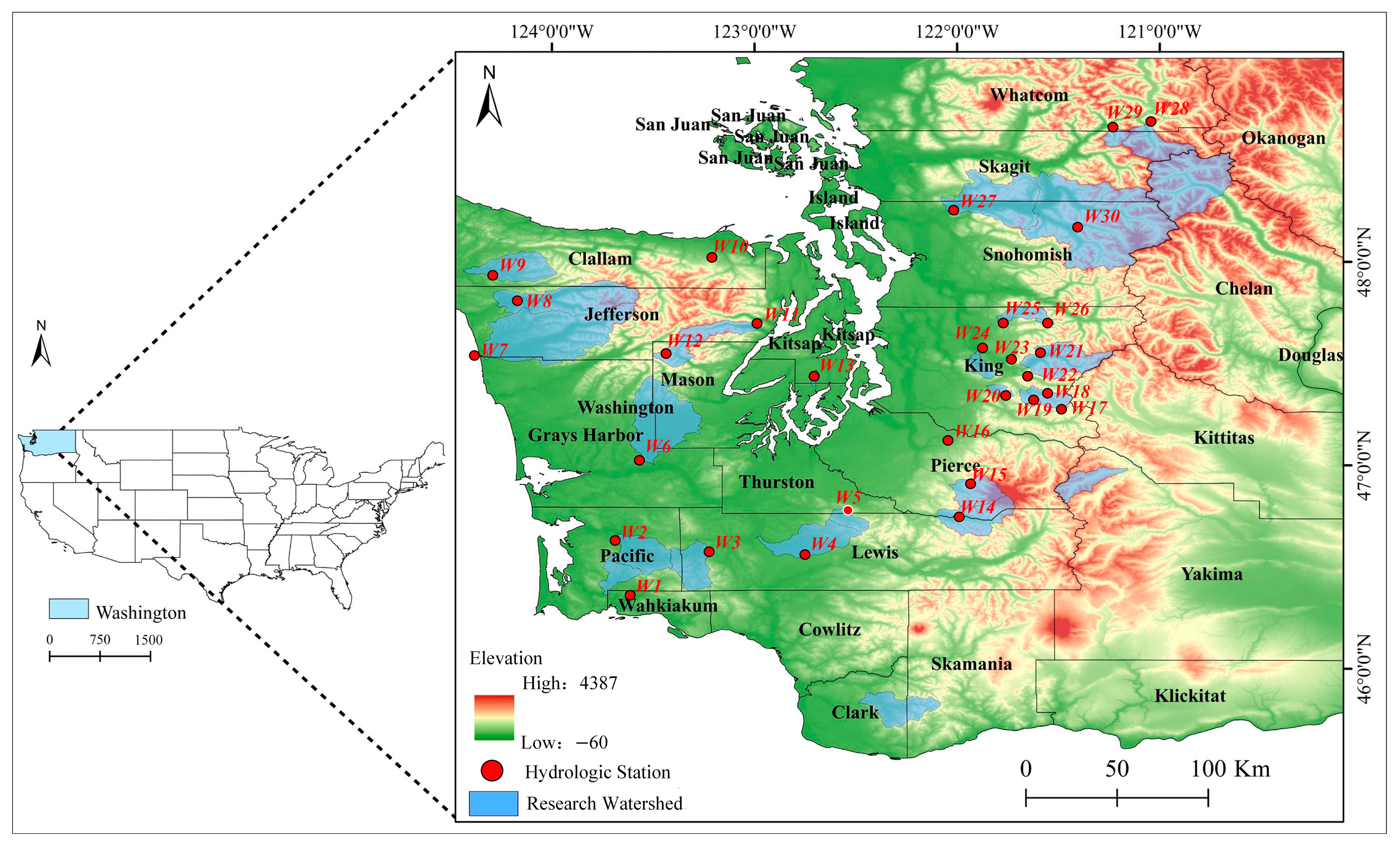
2.1. Research Area and Data

This study evaluated the predictive ability of hydrological models based on 30 hydrological stations in Washington, USA (Figure 1), the details of 30 hydrological stations are shown in

Table 1. Details of selecting hydrological stations in Washington State for research.

Site	Hydrological Station Name	Latitude	Longitude
W1	Naselle River Near Naselle	46.37	−123.74
W2	Willapa River Near Willapa	46.65	−123.65
W3	Chehalis River Near Doty	46.62	−123.28
W4	Newaukum River Near Chehalis	46.62	−122.95
W5	Skookumchuck River Near Vail	46.77	−122.59
W6	Satsop River Near Satsop	47.00	−123.49
W7	Queets River Near Clearwater	47.54	−124.32
W8	Hoh River At Us Highway 101 Near Forks	47.81	−124.25
W9	Calawah River Near Forks	47.96	−124.39
W10	Dungeness River Near Sequim	48.01	−123.13
W11	Duckabush River Near Brinnon	47.68	−123.01
W12	Nf Skokomish R Bl Staircase Rpds Nr Hoodsport	47.51	−123.33
W13	Huge Creek Near Wauna	47.39	−122.70
W14	Nisqually River Near National	46.75	−122.08
W15	Puyallup River Near Electron	46.90	−122.04
W16	South Prairie Creek At South Prairie	47.14	−122.09
W17	Cedar River Below Bear Creek Near Cedar Falls	47.34	−121.55
W18	Cedar River Near Cedar Falls	47.37	−121.63
W19	Rex River Near Cedar Falls	47.35	−121.66
W20	Taylor Creek Near Selleck	47.39	−121.85
W21	Middle Fork Snoqualmie River Near Tanner	47.49	−121.65
W22	Sf Snoqualmie River At Edgewick	47.45	−121.72
W23	Sf Snoqualmie River At North Bend	47.49	−121.79
W24	Raging River Near Fall City	47.54	−121.91
W25	North Fork Tolt River Near Carnation	47.71	−121.79
W26	South Fork Tolt River Near Index	47.71	−121.60
W27	Nf Stillaguamish River Near Arlington	48.26	−122.05
W28	Thunder Creek Near Newhalem	48.67	−121.07
W29	Newhalem Creek Near Newhalem	48.66	−121.24
W30	Sauk River Ab Whitechuck River Near Darrington	48.17	−121.47

. Washington is located on the continent’s west coast between latitudes 40 and 60 degrees. The western coastal region has a temperate marine climate with moderate temperatures and high precipitation, with an annual average rainfall of over 1000 mm. The eastern inland region has a semiarid climate with lower precipitation, with an annual average rainfall of around 250–500 mm. Due to the mountainous areas in Washington, winter precipitation often occurs in the form of snow, which melts in spring and becomes a critical water resource for irrigation, urban water supply, and hydropower. The hydrological stations selected for this study are mainly concentrated in western Washington state, classified as temperate marine climate (Cfb) according to the Koppen climate classification, with moderate temperatures and high precipitation, with an average annual rainfall of over 1000 mm [30].

Each watershed includes 25 years (1980–2004) of hydrometeorological data, which are divided into a model training period (1980–1999) and a validation period (2000–2004). The data are sourced from the US CAMLES dataset (https://gdex.ucar.edu/dataset/camels.html, accessed on 20 January 2023), which includes daily sunshine duration, daily precipitation, daily streamflow, daily maximum and minimum temperatures, as well as the elevation, latitude, and atmospheric pressure of the watersheds. Potential evapotranspiration (PET) is an essential input for hydrological models [31], but various methods exist to calculate it. In this study, the FAO-56 Penman-Monteith method is used as a reference [32,33], and daily reference crop evapotranspiration is calculated based on data such as daily sunshine duration, daily maximum and minimum temperatures, atmospheric pressure, elevation, and latitude.

2.2. Models and Methods

2.2.1. Introduction to Hydrological Models

Chiew simplified the HYDROLOG and MODHYDROLOG models and proposed the daily conceptual hydrological model SIMHYD [34]. The advantages of this model are its few input parameters, simple principles and structure, and good accuracy and applicability. The original SIMHYD model does not include a snowmelt module, which may lead to significant errors in simulating snowmelt dominated watershed models.

The SIMHYD_Snow model incorporates a snowmelt module, Snowmelt [35], into the SIMHYD model (Figure 2). This module divides daily precipitation into rainfall and snowfall based on maximum and minimum temperatures and then calculates daily snowmelt using the degree day factor method. The SIMHYD_Snow model has 11 parameters, including maximum infiltration capacity, maximum soil moisture content, actual evapotranspiration parameters, and groundwater recharge parameters. This study used a genetic algorithm for parameter calibration to achieve the best fit between the model and observed data, with the root mean square error (RMSE) set as the objective function.

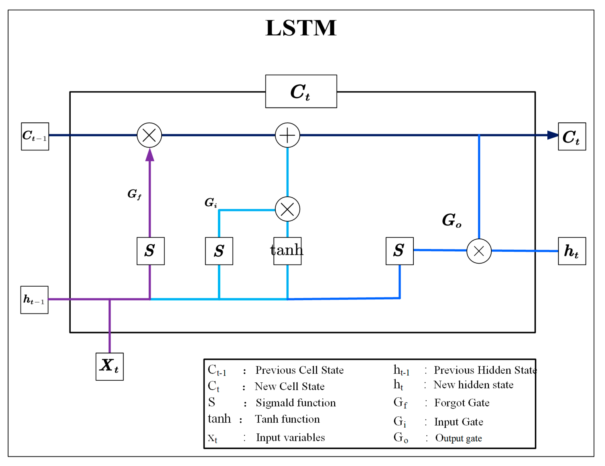
2.2.2. Introduction to LSTM Model

LSTM is a recurrent neural network (RNN) model widely used to classify, process, and predict time series data. In terms of long term memory, LSTM outperforms RNN due to its unique architecture, which overcomes the limited memory capacity issue in RNN.

The LSTM model consists of recursively connected memory cells, each equipped with a cell state, forget gate, input gate, output gate, and hidden state (Figure 3). The cell state stores and transmits information, while the forget gate is responsible for discarding certain information from the previous time step’s cell state. The input gate updates and stores important information in the cell state. The output gate extracts information into the hidden state at the current time step, which serves as the model’s output at each time step.

In this study, the LSTM model was constructed using the Deep Learning Toolbox in MATLAB. In order to optimize the structure and performance of the model and obtain the best prediction results, the model parameters were set as shown in

Table 2. LSTM Model Parameter Settings.

Parameter	Setting Values	Parameter	Setting Values
Number of hidden units	32	Abandonment rate	0.4
Maximum Number of Iterations	300	Gradient truncation threshold	1
optimizer	Adam	Learning rate reduction cycle	200
Batch size	32	Learning rate reduction factor	0.1
Initial learning rate	0.005

(The selected parameter set demonstrates exemplary performance in terms of computational efficiency and model stability, facilitating practical training and optimization of the model).

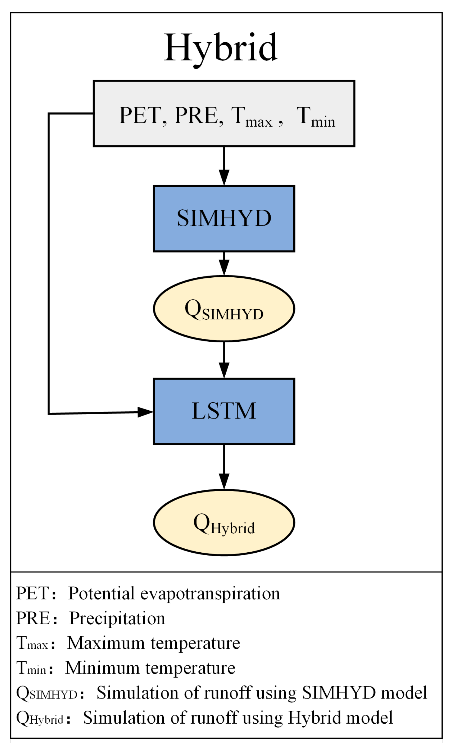
2.2.3. Combined Model Hybrid

In this study, a novel approach is proposed to utilize the output of the SIMHYD model as input for the LSTM model to simulate streamflow. Figure 4 shows primary meteorological data (including potential evapotranspiration PET, precipitation PRE, maximum temperature Tmax, and minimum temperature Tmin) that are input into the SIMHYD model to calculate the runoff. Then, the output of the SIMHYD model is used as input for the LSTM model to obtain the simulated streamflow of the combined model. Detailed information on the variables is provided in

Table 3. Model Input and Output Variable Settings.

Model	Input	Output	Target
SIMHYD	PRE, Tmax, Tmin, PET	Qsimhyd	Qobs
LSTM	PRE, Tmax, Tmin, PET	Qlstm	Qobs
Hybrid	PRE, Tmax, Tmin, PET, Qsimhyd	Qhybrid1	Qobs

.

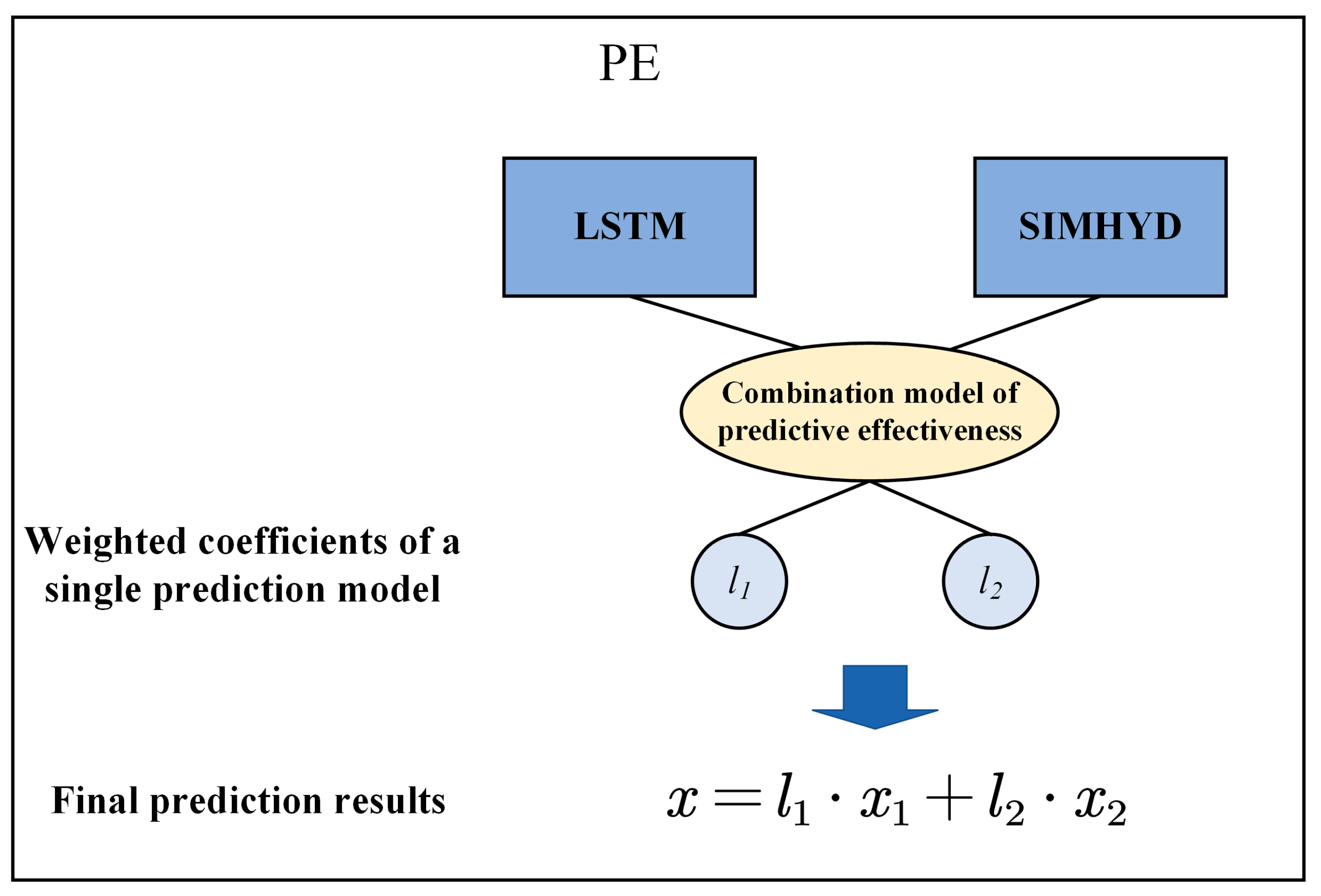
2.2.4. Combined Forecasting Model for Dynamic Prediction Effectiveness

The Combination Prediction Model for Prediction Effectiveness

The combination forecasting model based on predictive validity utilizes the practical information provided by various forecasting methods, calculated in an appropriate weighted average form to obtain the combined model. In order to improve the accuracy of the combined forecasting model, this study focuses on two aspects: firstly, the determination of the weighted average coefficients for each individual forecasting model in the combined forecasting model, and secondly, the examination of whether the combined forecasting results are superior to those of the individual forecasting models. The Combination prediction model for prediction effectiveness (PE) selected in this study utilizes the mean of predictive accuracy and the mean square deviation reflecting the degree of dispersion to construct an optimal calculation model for weighted coefficients through linear programming (Figure 5). It overcomes the influence of the deviation in forecasting results due to the different dimensions of the indicator sequences in the ordinary combined forecasting model, thereby improving the forecasting accuracy. Moreover, the model is intuitive, computationally concise, and possesses practical application value.

The measured runoff sequence is {xt, t = 1, 2, 3 … N}, and there are m individual prediction models predicting it. x_it is the water quality prediction value of the i-th single-item prediction method at time t, where i ranges from 1 to N. e_it is the relative error between the measured runoff and the predicted runoff by the i-th prediction method at time t, i.e., e_it = (x_i − x_it)/xi. Let A_it = e − |e_it|, and 0 ≤ e_it ≤ 1, then A_it is the prediction accuracy of the i-th runoff prediction model at time t, obviously 0 ≤ A_it ≤ 1.

Let $\widehat{x}$_t be the combined prediction value of x_t, then we have:

$$\widehat{x}=l_1{x}_{1t}+l_2{x}_{2t}+\dots +l_m{x}_{mt}, l_1, l_2,\dots ,l_m$$

(1)

ln is the weighted coefficient of a single prediction model and has:

$${\displaystyle \sum _{j=1}^m{l}_j=1, l_j\ge 0, j=1,\dots ,m}$$

(2)

If A_t and e_t are the combined prediction accuracy and relative error at time t, then there are:

$$A_t={\displaystyle \sum _{i=1}^m{l}_i{A}_{1t}+l_2{A}_{2t}+\dots +l_m{A}_{mt}=1-}\left|e_t\right|=1-\left|{\displaystyle \sum _{i=1}^m{l}_i{e}_{it}}\right|$$

(3)

The effectiveness of the i-th prediction model is:

$$E\left(A_i\right)={\displaystyle \sum _{t=1}^N{Q}_{it}{A}_{it}}$$

(4)

where Q_it represents the weight coefficient of the accuracy A_it of the i-th prediction method at time t on the sample interval and has:

$${\displaystyle \sum _{t=1}^N{Q}_{it}=1,Q_{it}\gg 0, t=1,2,\dots ,N}$$

(5)

Because prior information is not clear, Q is taken as 1/N. So there are:

$$E\left(A_i\right)={\displaystyle \frac{1}{N}}{\displaystyle \sum _{i=1}^N{A}_t}$$

(6)

The prediction validity sequence values for each individual model. The prediction accuracy sequence of the combined prediction model satisfies:

$$E\left(A\right)={\displaystyle \sum _{i=1}^m{l}_{i}E\left(A_i\right)=\frac{1}{N}}{\displaystyle \sum _{t=1}^N{A}_t}$$

(7)

The solution formula for σ²(A) is:

$$\begin{array}{cc}\hfill \sigma \left(A\right)=\sqrt{D\left(A\right)}& =\sqrt{\frac{1}{N}{\displaystyle \sum _{t=1}^N{\left(A_t-E\left(A\right)\right)}^2}}\hfill \\ & ={\left\{{\displaystyle \sum _{i=1}^m{l}_i^2}{\sigma }^2\left(A_i\right)+{\displaystyle \sum _{i\ne j}{l}_i{l}_j{\rho }_{ij}}\sigma \left(A_i\right)\sigma \left(A_j\right)\right\}}^{{\displaystyle \frac{1}{2}}}\hfill \end{array}$$

(8)

Among ρ_ij is the correlation coefficient between the prediction accuracy of the i-th runoff prediction model and the prediction accuracy of the j-th runoff prediction model, namely:

$${\rho }_{ij}={\displaystyle \frac{1}{N}}\left\{{\displaystyle \sum _{t=1}^N\left[A_{ij}-E\left(A_i\right)\right]\cdot }\left[A_{ij}-E\left(A_i\right)\right]/\left[\sigma \left(A_i\right)\sigma \left(A_j\right)\right]\right\}$$

(9)

E(A) represents the average prediction accuracy of the combination prediction method at different times, with larger values leading to higher accuracy: σ(A) represents the stability of the prediction accuracy sequence of the combination prediction model, and the smaller the value, the better the model.

The effectiveness index of the combination prediction model is defined as:

$$S\left(l_1,l_2,\dots ,l_m\right)=E\left(A\right)\left[1-\sigma \left(A\right)\right]$$

(10)

In the equation, S represents the fitting between the predicted model and the measured runoff. The larger S, the better the linear fitting between the two, and the higher the effectiveness of the predicted results.

The combination prediction model based on prediction effectiveness is:

$$\begin{gathered} \max S=\left[{\displaystyle \sum _{i=1}^m{l}_{i}E\left(A_i\right)\cdot \left\{1-{\left[{\displaystyle \sum _{i=1}^m{l}_i^2{\sigma }^2\left(A_i\right)+{\displaystyle \sum _{i\ne j}{l}_i{l}_j{\rho }_{ij}\sigma \left(A_i\right)\sigma \left(A_j\right)}}\right]}^{\frac{1}{2}}\right\}}\right] \\ \mathrm{s}.\mathrm{t}.\left\{\begin{array}{c}{\displaystyle \sum _{i=1}^m{l}_i=1}\\ l_i\ge 0,i=1,2,\dots ,m\end{array}\right\} \end{gathered}$$

(11)

In this system of equations, as long as the predicted values x_it of m prediction methods at different times are calculated, the definition equation can be used to calculate (E)A_i, (σ)A_i, (σ)²A_i and then to calculate ρ_ij. Using the Lagrange multiplier method, the calculated values of (E)A_i, (σ)A_i, (σ)²A_i, ρ_ij are used to calculate the weighting coefficients l₁, l₂,… for various prediction models, The functions of l_m and l_n are used to find l₁, l₂, … that meet the maximum value requirements of the formula maxS, The weight values of l_m and l_n.

A Combined Forecasting Model for Dynamic Prediction Effectiveness

In order to further enhance the prediction accuracy of the combination prediction model based on predictive validity, this study proposes an improved Combined Forecasting Model for Dynamic Prediction Effectiveness. As shown in Figure 6, we set 5 unit times as onetime step T and input T into the predictive validity hybrid model to calculate the individual model weight values corresponding to this time segment, which are then used to compute the combined model simulation results for the time point after T. (The shorter the set time interval, the higher the accuracy of the model, although it comes at the cost of increased computational time. In our testing, it was observed that setting the time interval to 5 units yielded more favorable simulation results while requiring less computational time). Subsequently, the initial and final values of period T are incremented by 1, and the combination prediction model is re-input for the calculation to obtain the weighted coefficients of the individual models for the time point after T. This process is iterated until the last time point, thus computing the individual model weight values corresponding to all time points.

2.2.5. Model Evaluation Indicators

This study selects the NSE to evaluate model performance. The NSE is a commonly used index proposed by hydrologist J.R. Nash in 1970. It measures the fit between model simulation results and actual observed values, assessing model simulation performance [36]. A value of NSE closer to 1 indicates a better fit of the model to the observed values. NSE is calculated using the following formula:

$$NSE=1-{\displaystyle \frac{{\displaystyle \sum {(Q_m-Q_{obs})}^2}}{{\displaystyle \sum {(Q_{obs}-\overline{Q_{obs}})}^2}}}$$

(12)

In the equation, Q_m represents the modeled runoff (m³/s), and Q_obs represents the observed runoff (m³/s).

The Taylor diagram is a graphical representation method used to compare the correlation, bias, and standard deviation between model outputs and observed data. It shows the performance of different model predictions in terms of correlation, variance, and standard deviation compared to observed data, helping to evaluate the accuracy and bias of the models. The Taylor diagram is typically presented in a polar plot, with the standard deviation and correlation coefficient of the observed values as axes and the standard deviation and correlation coefficient of the model predictions plotted as points, visually comparing the differences between the models and observed data. A Taylor diagram typically displays three evaluation metrics: Correlation Coefficient, Standard Deviation, and Root Mean Square Error (RMSE).

The Correlation Coefficient measures the strength and direction of the linear relationship between model predictions and observed values. It is calculated as:

$$R={\displaystyle \frac{{\displaystyle \sum _{i=1}^N\left(x_i-\overline{x}\right)}\left(y_i-\overline{y}\right)}{\sqrt{{\displaystyle \sum _{i=1}^N{\left(x_i-\overline{x}\right)}^2}}\sqrt{{\displaystyle \sum _{i=1}^N{\left(y_i-\overline{y}\right)}^2}}}}$$

(13)

In the equation, N is the total number of data points, x_i and y_i are individual data points for the two variables, x and y are the means of the two variables.

The Standard Deviation measures the variability or spread of data points around the mean. In the Taylor diagram, it represents the dispersion of model predictions and observed values. It is calculated as:

$$\sigma =\sqrt{{\displaystyle \frac{1}{N}}{\displaystyle \sum _{i=1}^N{\left(x_i-\overline{x}\right)}^2}}$$

(14)

In the equation, N is the total number of data points, x_i represents each data point, x is the mean value of the data points.

The Root Mean Square Error is a measure of the differences between values predicted by a model and the observed values. It is calculated as:

$$RMSE=\sqrt{{\displaystyle \frac{1}{N}}{\displaystyle \sum _{i=1}^N{\left(y_i-\widehat{y}\right)}^2}}$$

(15)

In the equation, N is the total number of data points, y_i represents the observed values, y_i represents the model predicted values.

3. Results

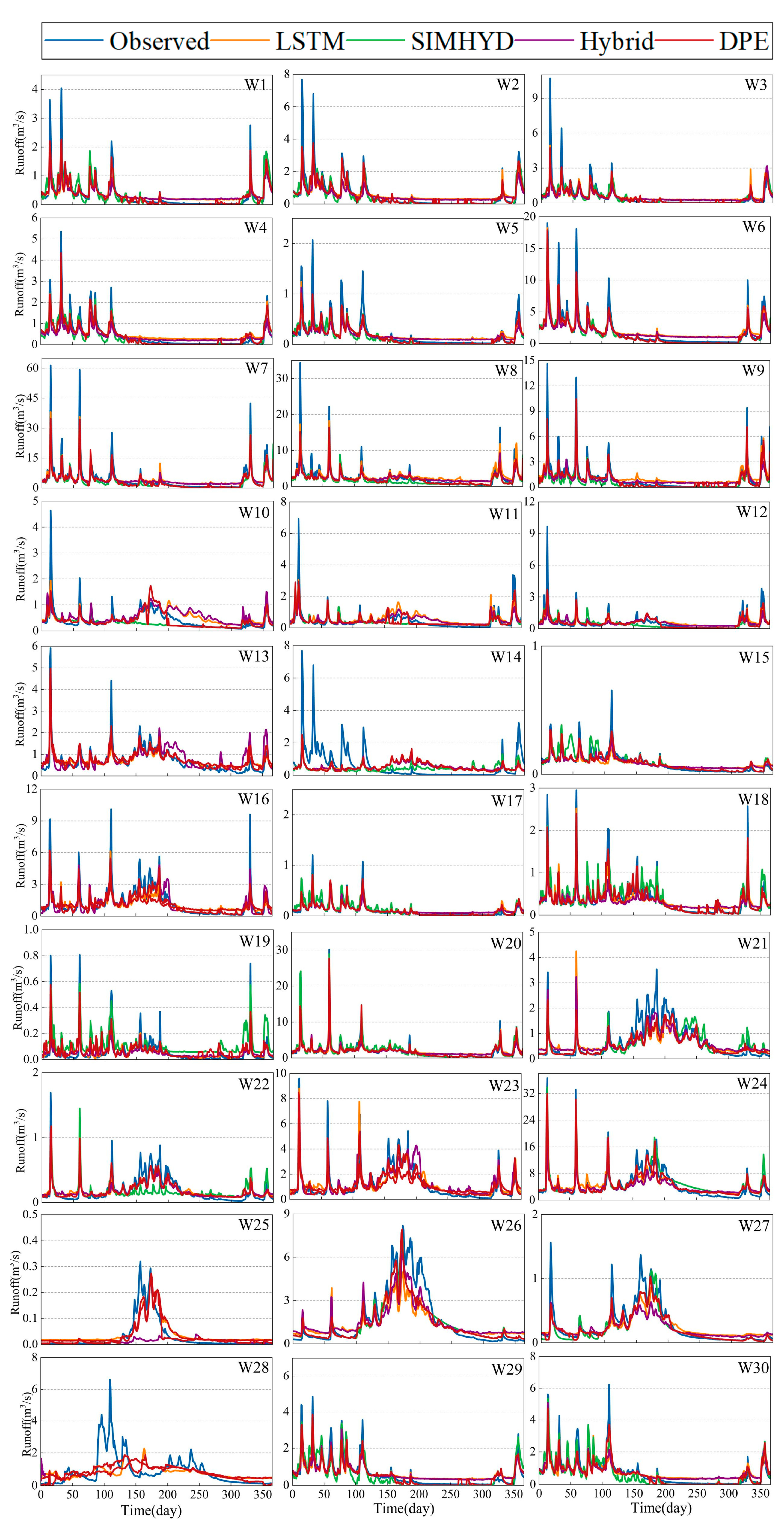
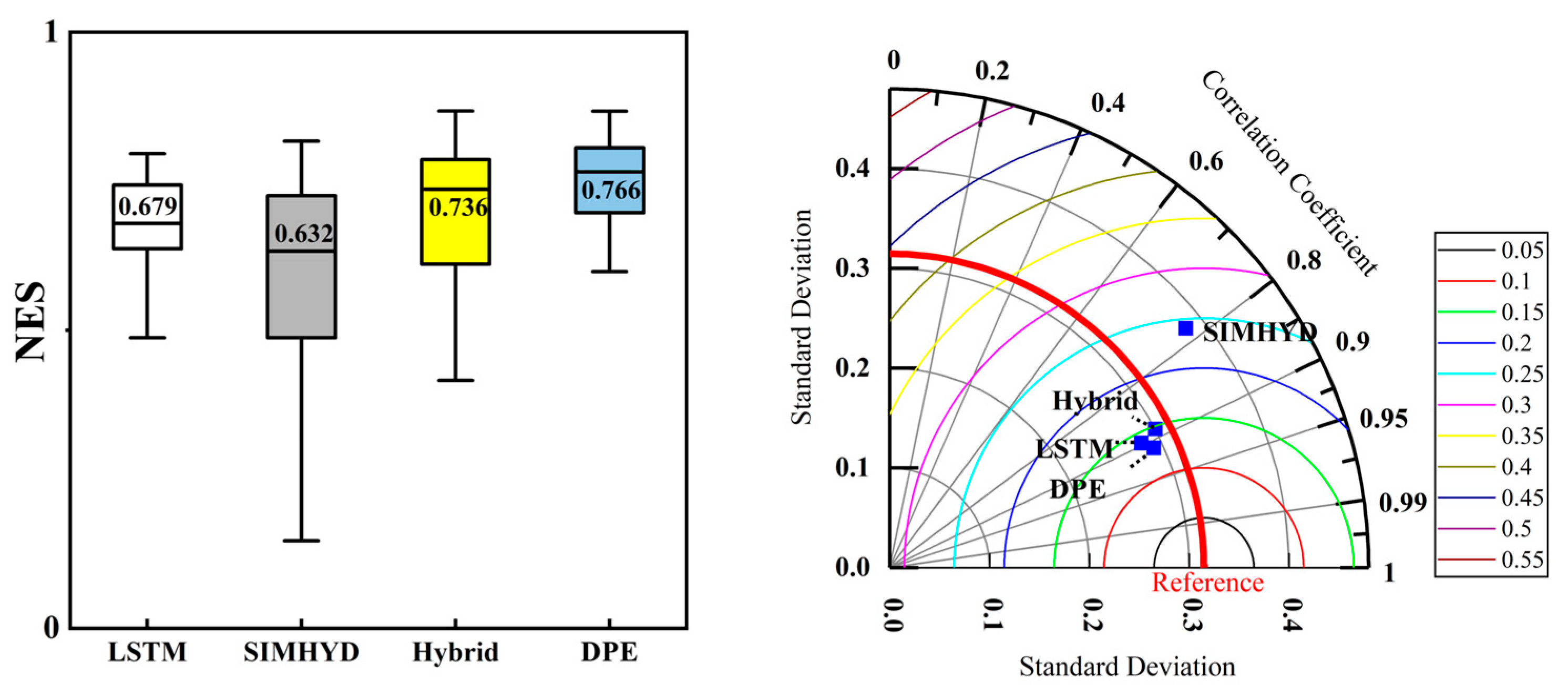
3.1. Model Runoff Simulation Capability

Figure 7 is a line graph of the runoff simulation results for a single model and two combined models of 30 hydrological stations in Washington State in 2000 (validation period from 2000 to 2004, all displayed will affect the appearance, so only the results from 2000 are shown).

Table 4. NES value and R2 of runoff simulation results during model validation period.

	NES				R2
	LSTM	SIMHYD	Hybrid	DPE	LSTM	SIMHYD	Hybrid	DPE
W1	0.751	0.783	0.752	0.853	0.897	0.788	0.921	0.928
W2	0.764	0.819	0.738	0.850	0.901	0.830	0.912	0.922
W3	0.680	0.719	0.688	0.779	0.779	0.727	0.817	0.821
W4	0.774	0.801	0.595	0.840	0.894	0.836	0.793	0.931
W5	0.742	0.756	0.715	0.821	0.853	0.802	0.873	0.881
W6	0.795	0.793	0.752	0.889	0.891	0.805	0.914	0.919
W7	0.778	0.820	0.755	0.858	0.869	0.855	0.872	0.900
W8	0.772	0.747	0.673	0.789	0.853	0.798	0.850	0.854
W9	0.777	0.545	0.688	0.817	0.851	0.664	0.853	0.857
W10	0.542	0.274	0.505	0.697	0.558	0.352	0.538	0.719
W11	0.535	0.696	0.473	0.767	0.549	0.735	0.536	0.804
W12	0.618	0.671	0.542	0.786	0.656	0.678	0.644	0.816
W13	0.717	0.546	0.674	0.788	0.792	0.553	0.790	0.838
W14	0.667	0.635	0.610	0.766	0.715	0.648	0.727	0.816
W15	0.757	0.727	0.752	0.854	0.906	0.750	0.910	0.931
W16	0.729	0.708	0.677	0.815	0.810	0.720	0.837	0.851
W17	0.771	0.779	0.759	0.883	0.898	0.797	0.911	0.909
W18	0.751	0.700	0.692	0.856	0.823	0.761	0.829	0.869
W19	0.677	0.063	0.593	0.698	0.719	0.613	0.804	0.812
W20	0.734	0.766	0.708	0.870	0.841	0.828	0.827	0.878
W21	0.697	0.339	0.732	0.813	0.751	0.469	0.821	0.855
W22	0.643	0.527	0.697	0.813	0.676	0.549	0.803	0.854
W23	0.554	0.501	0.488	0.606	0.571	0.503	0.604	0.624
W24	0.700	0.774	0.670	0.858	0.752	0.782	0.822	0.870
W25	0.517	0.513	0.570	0.612	0.539	0.001	0.573	0.632
W26	0.665	0.705	0.741	0.802	0.740	0.730	0.860	0.893
W27	0.678	0.720	0.676	0.828	0.745	0.729	0.773	0.860
W28	0.082	0.208	0.132	0.288	0.115	0.218	0.133	0.297
W29	0.713	0.788	0.783	0.855	0.894	0.795	0.911	0.923
W30	0.704	0.788	0.736	0.844	0.856	0.788	0.899	0.906

shows the NES and R2 values of the simulation results during the validation period for four models at 30 hydrological stations. The results showed that compared to individual models and direct combination models, the DPE model demonstrated better runoff simulation capabilities at all 30 stations, with good simulation results for both low and peak runoff. It is worth mentioning that the results of the four models at hydrological station W28 did not meet expectations, which may be due to the lack of some rainfall data during the validation period of the station.

Figure 8 presents the boxplots of evaluation metrics for the simulated runoff results from the individual models and two hybrid models. The results indicate that, compared to the independent SIMHYD model, the median NSE of the validation period for the Hybrid model and the DPE model have improved by 16.5% and 21.2%, respectively. That demonstrates a significant enhancement in the runoff modeling capabilities of the two hybrid models, with the DPE model exhibiting more robust runoff modeling capabilities. Additionally, the runoff simulation stability of the two hybrid models has significantly improved compared to the SIMHYD model. Furthermore, the Taylor diagrams of the models reveal that the hybrid models and the DPE model exhibit higher correlation coefficients, lower root mean square errors, and more minor standard deviations than the SIMHYD model.

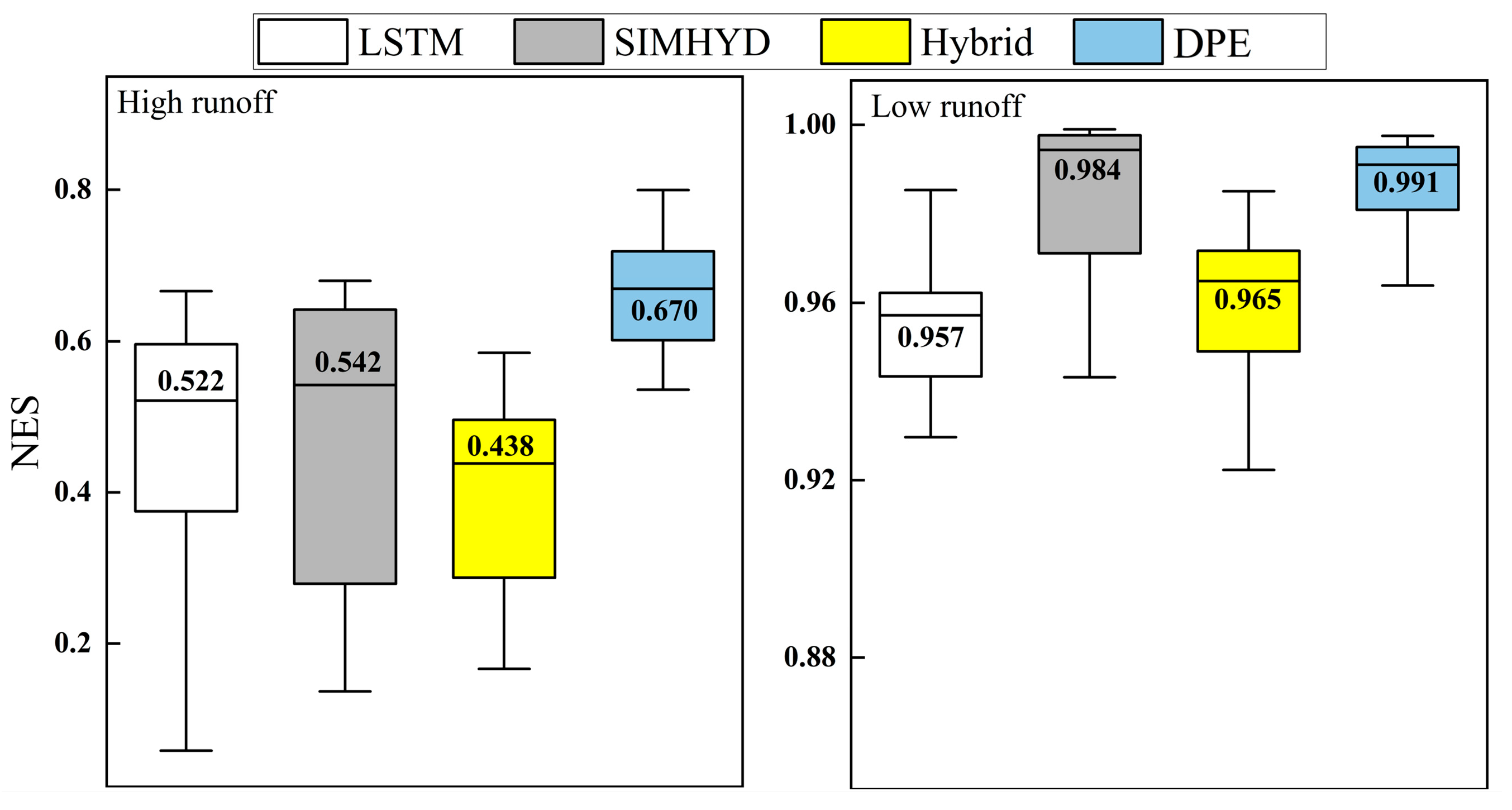
3.2. The Ability of the Model to Simulate Extreme Traffic

The key to whether the hybrid model can better forecast flood and drought disasters lies in whether the ability of the hybrid model to simulate extreme flows has been improved compared to that of the individual models [37]. In this study, the top 25% of observed runoff data during the validation period is selected as the relatively high flow data, while the bottom 25% is selected as the relatively low flow data for the basin. A boxplot of evaluation metrics for the model’s simulation of extreme flows is then plotted (Figure 9).

The models exhibit significant differences in their ability to simulate high flows, with the DPE hybrid model demonstrating the best model performance. Compared to the SIMHYD model, the DPE model shows a 23.6% increase in the median NSE for high flow simulation. Compared to the LSTM model, the DPE model exhibits a 28.4% increase in the median NSE of simulated high flows, and the length of the boxplot for this model is shorter, indicating more excellent stability in simulating high flows. In simulating low flows, both the individual models and the hybrid model perform very well. However, compared to the SIMHYD model, the DPE hybrid model shows significantly improved stability in simulating low flows. These results indicate that the DPE model outperforms the individual models in simulating extreme flows.

4. Discussion

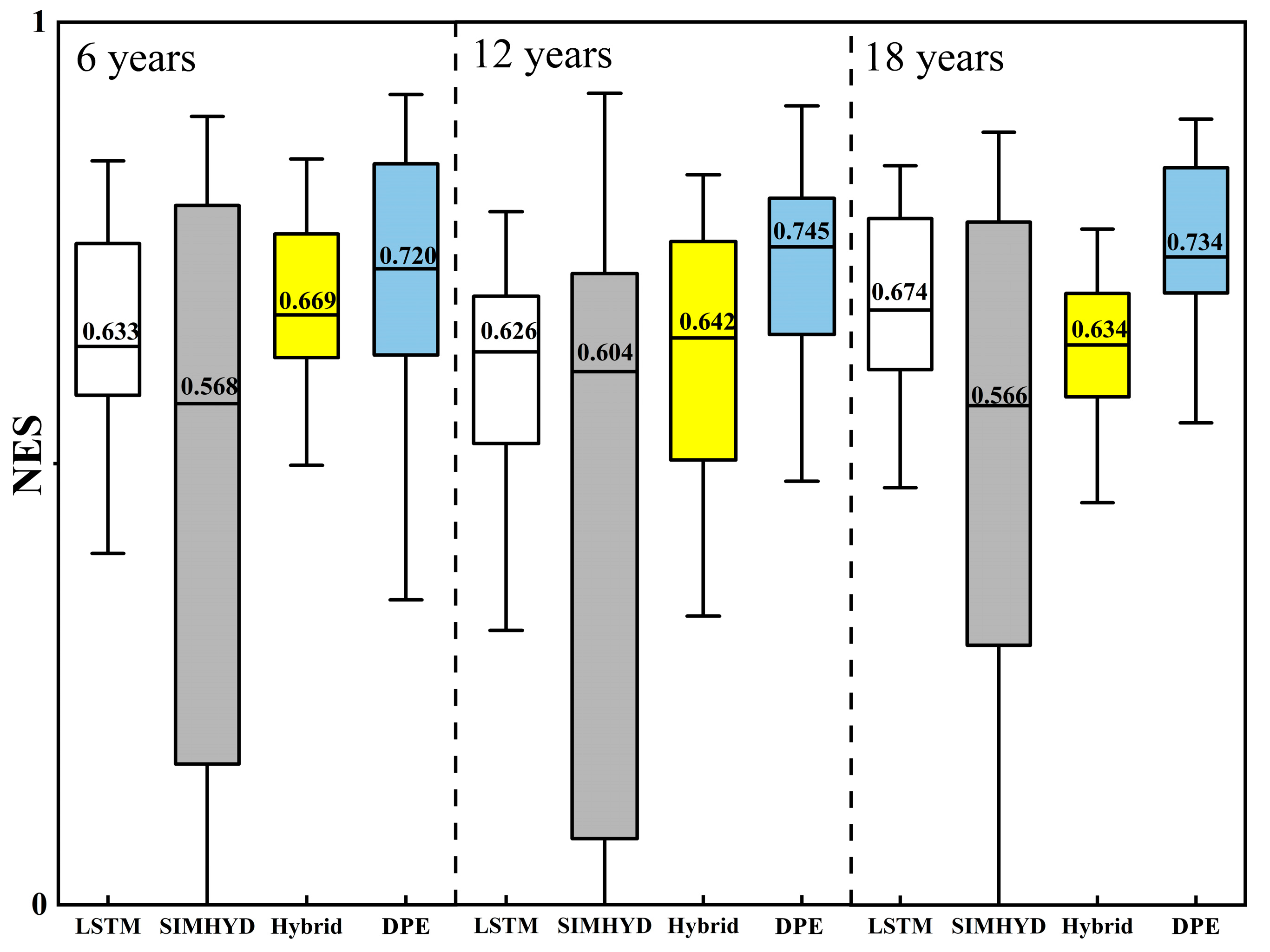
4.1. The Predictive Performance of the Model Under Different Training Periods of Length

The training period length of the runoff prediction model is an important consideration affecting model performance [38]. An excessively long training period may lead to overfitting the model to the training data [39], resulting in poor performance on new data, while a too short training period may prevent the model from fully capturing the data’s features, thereby affecting the model’s accuracy and stability [40]. Determining the appropriate training period length is crucial for establishing an effective runoff prediction model. Therefore, this study analyzed the impact of three different training period lengths on model performance and plotted the evaluation metrics in box plots for training periods of 6 years, 12 years, and 18 years (see Figure 10).

Selecting an appropriate training period length enhances the precision and efficiency of model predictions. As depicted in Figure 9, the predictive performance of the DPE model surpasses that of the standalone model in all three scenarios, further highlighting the superior predictive ability of this coupled model in runoff prediction. Comparing the model prediction outcomes for validation period lengths of 6 years and 12 years, it is evident that when the training period is set to 12 years, the performance of all hybrid models strengthens significantly. That indicates that the models needed more data for learning during the 6-year training period. In shorter training periods, models may struggle to capture the intricate patterns and trends within the data. Extending the training period can provide the model with more data to learn from, thereby increasing the accuracy of predictions [41].

Comparing the model prediction results for training period lengths of 12 years and 18 years, the SIMHYD model and the combined prediction model DPE exhibit lower NSE values when the training period is set to 18 years compared to the 12-year training period. That may be due to the models overfitting the training data, resulting in a decreased generalization ability on new data [42]. A more extended training period may cause the model to overly rely on noise or specific patterns within the training data, potentially overlooking genuine trends and patterns, which could lead to poor predictive performance on new data [43].

In summary, setting an appropriate length for the training period helps the model learn the patterns and trends within the data, thereby enhancing its generalization ability on new data. Additionally, it can reduce the risk of the model overfitting the training data, improve training efficiency, and enable the model to make more accurate predictions.

4.2. The Runoff Simulation Ability of Individual and Combined Models

Compared to individual models, the combined model exhibits more robust runoff simulation capability, which confirms Mohammadi’s [44] conclusion that combining hydrological models and machine learning models can enhance the accuracy of runoff simulation. The advantage of the combined model may stem from the complementarity of hydrological and machine learning models. Hydrological models utilize physical principles and parameter estimation based on observed data to simulate runoff processes, offering high interpretability and reliability. Machine learning models enhance prediction accuracy by learning associations in data, particularly excelling in handling large amounts of nonlinear data. Combining the two can overcome their respective limitations and achieve a more accurate and robust runoff simulation.

Comparing our research with similar hydrological simulation studies in other regions, we can find some similar and different conclusions. For example, Zarei et al. [45] found that simulating high traffic presents challenges, and even with the use of composite models, the improvement obtained is very limited. This is consistent with our findings that although the composite model DPE exhibits good simulation ability for high traffic, underestimation of high traffic still occurs. Sezen and Sraj [46] also acknowledged the ability of combined models to simulate low traffic, but their research overestimated low traffic. When conducting research on selecting training period lengths, Sharma and Kumari [47] found similar conclusions to ours, suggesting that an appropriate training period length can yield better simulation results. Compared to previous research on runoff simulation combination models, such as the FT-LSTM model proposed by Sonali et al. [48] that combines Fourier transform and LSTM models (12.0%), and the Conv TALSTM model proposed by Liu et al. [49] that introduces convolution kernels and attention mechanisms into LSTM networks (5.1%), the DPE model has a greater improvement on individual models (12.8%).

Although the combined model performs well in runoff simulation, it still faces challenges and limitations. Specifically, challenges primarily focus on model structure design and prediction accuracy. Firstly, the reasonable combination of hydrological and machine learning models is crucial. According to Lee [50] and others, designing a combined model requires considering the integration of the physical principles of hydrological models and the data-driven capabilities of machine learning models to improve simulation performance. Unreasonable model structure design may lead to reduced performance. For example, the Hybrid model only inputs primary hydrological data and the output of the SIMHYD model into the LSTM model, which may result in the model’s inability to accurately capture the characteristics and patterns of hydrological processes, leading to inaccurate predictions. Secondly, the complexity of model inputs and the issue of overfitting. Research by Kavetski [51] and others indicates that machine learning models are prone to overfitting when there are too many input variables, meaning they excessively fit the training data and lose generalization ability. In such cases, the model’s performance in simulating extreme flows may need improvement. Therefore, the complexity of model inputs may be one of the reasons for the decline in the performance of the Hybrid model during the validation period. In summary, a reasonable model structure design for hybrid models and avoiding overfitting are directions for future improvement.

In order to enhance the runoff simulation capability of the combined prediction model based on prediction effectiveness, this paper proposes the improved model DPE. The model can calculate the weighted coefficients of the individual model for the next step based on the runoff simulation results of the previous step. The results in Figure 7 and Figure 8 indicate that, compared to the individual model, the runoff simulation capability of the combined model DPE is more robust. In addition, the DPE model demonstrates superior performance in simulating extreme flow events, indicating its capability to capture and forecast extreme flow conditions accurately. That further emphasizes the robustness and reliability of the improved combination forecasting model in handling extreme flow scenarios, which is crucial for enhancing the overall predictive effectiveness of the model in hydrological applications. When evaluating the model performance, we utilized a subset of data from the US CAMELS dataset and did not assess the model’s ability to simulate data from other regions. That may result in a slightly lower representation of the model evaluation outcomes. In future work, we plan to evaluate the model performance using data from various regions to enhance the generalizability of our findings.

4.3. Limitations and Future Challenges

Data reliability and continuity: The model has strict requirements for the accuracy of input data, and the model requires that the input data should be continuous and real. Continuous data can provide the model with better learning ability, and the model can only demonstrate better simulation ability during the validation period.

The ability to simulate high flow: Hydrological models provide better response to high flow, but still underestimate it. In the future, models for extreme flow need to have faster and more accurate response capabilities.

5. Conclusions

In order to improve the runoff simulation capability of traditional hydrological models, this study combines the machine learning model LSTM with the hydrological model SIMHYD. Two different hybrid models were constructed, and the runoff data of 30 watersheds in Washington State were simulated. The runoff simulation effects of the two model combination methods were evaluated, and further validation of the model’s performance in simulating high and low flows was conducted. Based on the experimental results, the following main conclusions were drawn:

• The hybrid model has better runoff simulation capability than traditional hydrological models, significantly improving the median NSE during the validation period.
• The hybrid model DPE performs better in simulating extreme flow conditions than the individual model, contributing to better early warning of floods and droughts.
• The overall improvement in the hybrid model’s performance demonstrates the hybrid model’s ability to improve runoff simulation accuracy. Although this study only selected river basins in Washington State, and the results may not be generalized to other basins, the excellent hybrid approach provided can be used as a reference for other regions. However, there are still some issues that need to be addressed in our future research:

  (1)

  Further optimize the model combination method of the hybrid model to improve its learning ability.

  (2)

  Explore the runoff simulation capability of hybrid models in different climatic regions.

  (3)

  Enhance the model’s ability to simulate high flows and improve its capability to forecast flood disasters.

In order to more intuitively demonstrate the enhancement of the runoff simulation capability of the hybrid model over individual models, this study only selected the LSTM model and the SIMHYD model for combined analysis, which indeed needs a certain level of representativeness. This aspect will be further improved and modified in future work, where updated individual models and more efficient model combination methods will be used for evaluation.

References

1. Doycheva, K.; Horn, G.; Koch, C.; Schumann, A.; König, M. Assessment and weighting of meteorological ensemble forecast members based on supervised machine learning with application to runoff simulations and flood warning. Adv. Eng. Inform. 2017, 33, 427–439. [Google Scholar] [CrossRef]
2. Kreibich, H.; Thieken, A.H.; Petrow, T.; Müller, M.; Merz, B. Flood loss reduction of private households due to building precautionary measures—lessons learned from the Elbe flood in August 2002. Nat. Hazards Earth Syst. Sci. 2005, 5, 117–126. [Google Scholar] [CrossRef]
3. Blöschl, G.; Sivapalan, M. Scale issues in hydrological modelling: A review. Hydrol. Process. 1995, 9, 251–290. [Google Scholar] [CrossRef]
4. Wang, X.; Liu, T.; Yang, W. Development of a robust runoff-prediction model by fusing the rational equation and a modified SCS-CN method. Hydrol. Sci. J. 2012, 57, 1118–1140. [Google Scholar] [CrossRef]
5. Gebregiorgis, A.S.; Hossain, F. Understanding the dependence of satellite rainfall uncertainty on topography and climate for hydrologic model simulation. IEEE Trans. Geosci. Remote Sens. 2012, 51, 704–718. [Google Scholar] [CrossRef]
6. Burges, S.J. Streamflow prediction: Capabilities, opportunities, and challenges. Hydrol. Sci. Tak. Stock. Look. Ahead 1998, 5, 101–134. [Google Scholar]
7. Talei, A.; Chua LH, C. Influence of lag time on event based rainfall–runoff modeling using the data driven approach. J. Hydrol. 2012, 438, 223–233. [Google Scholar] [CrossRef]
8. Xiao, W.; Zhou, J.; Yang, J.; Mo, L.; Xu, Z.X.; Yang, Y.Q. Long-term runoff forecast in the middle and lower reaches of the Yangtze River based on machine learning. Water Resour. Power 2022, 40, 31–34+26. [Google Scholar] [CrossRef]
9. Nayak, P.; Venkatesh, B.; Krishna, B.; Jain, S.K. Rainfall-runoff modeling using conceptual, data driven, and wavelet based computing approach. J. Hydrol. 2013, 493, 57–67. [Google Scholar] [CrossRef]
10. Chang, C.W.; Dinh, N.T. Classification of machine learning frameworks for data-driven thermal fluid models. Int. J. Therm. Sci. 2019, 135, 559–579. [Google Scholar] [CrossRef]
11. Gharari, S.; Razavi, S. A review and synthesis of hysteresis in hydrology and hydrological modeling: Memory, path-dependency, or missing physics? J. Hydrol. 2018, 566, 500–519. [Google Scholar] [CrossRef]
12. Noble, W.S. What is a support vector machine? Nat. Biotechnol. 2006, 24, 1565–1567. [Google Scholar] [CrossRef]
13. Rigatti, S.J. Random forest. J. Insur. Med. 2017, 47, 31–39. [Google Scholar] [CrossRef]
14. Yin, C.; Zhu, Y.; Fei, J.; He, X. A deep learning approach for intrusion detection using recurrent neural networks. IEEE Access 2017, 5, 21954–21961. [Google Scholar] [CrossRef]
15. Yang, Y.; McVicar, T.R.; Donohue, R.J.; Zhang, Y.; Roderick, M.L.; Chiew, F.H.; Zhang, L.; Zhang, J. Lags in hydrologic recovery following an extreme drought: Assessing the roles of climate and catchment characteristics. Water Resour. Res. 2017, 53, 4821–4837. [Google Scholar] [CrossRef]
16. Siami Namini, S.; Namin, A.S. Forecasting economics and financial time series: ARIMA vs. LSTM. arXiv 2018, arXiv:1803.06386. [Google Scholar]
17. Amalou, I.; Mouhni, N.; Abdali, A. Multivariate time series prediction by RNN architectures for energy consumption forecasting. Energy Rep. 2022, 8, 1084–1091. [Google Scholar] [CrossRef]
18. Man, Y.; Yang, Q.; Shao, J.; Wang, G.; Bai, L.; Xue, Y. Enhanced LSTM model for daily runoff prediction in the upper Huai river basin, China. Engineering 2022, 24, 229–238. [Google Scholar] [CrossRef]
19. Kanai, S.; Fujiwara, Y.; Iwamura, S. Preventing gradient explosions in gated recurrent units. Adv. Neural Inf. Process. Syst. 2017, 30. [Google Scholar]
20. Hochreiter, S.; Schmidhuber, J. Long short-term memory. Neural Comput. 1997, 9, 1735–1780. [Google Scholar] [CrossRef]
21. Kim, C.; Kim, C.S. Comparison of the performance of a hydrologic model and a deep learning technique for rainfall-runoff analysis. Trop. Cyclone Res. Rev. 2021, 10, 215–222. [Google Scholar] [CrossRef]
22. Yuan, X.; Chen, C.; Lei, X.; Yuan, Y. Monthly runoff forecasting based on LSTM–ALO model. Stoch. Environ. Res. Risk Assess. 2018, 32, 2199–2212. [Google Scholar] [CrossRef]
23. Adnan, R.M.; Dai, H.-L.; Mostafa, R.R.; Parmar, K.S.; Heddam, S.; Kisi, O. Modeling multistep ahead dissolved oxygen concentration using improved support vector machines by a hybrid metaheuristic algorithm. Sustainability 2022, 14, 3470. [Google Scholar] [CrossRef]
24. Adnan, R.M.; Mostafa, R.R.; Dai, H.-L.; Heddam, S.; Kuriqi, A.; Kisi, O. Pan evaporation estimation by relevance vector machine tuned with new metaheuristic algorithms using limited climatic data. Eng. Appl. Comput. Fluid Mech. 2023, 17, 2192258. [Google Scholar] [CrossRef]
25. Okkan, U.; Ersoy, Z.B.; Kumanlioglu, A.A.; Fistikoglu, O. Embedding machine learning techniques into a conceptual model to improve monthly runoff simulation: A nested hybrid rainfall-runoff modeling. J. Hydrol. 2021, 598, 126433. [Google Scholar] [CrossRef]
26. Liu, J.; Yuan, X.; Zeng, J.; Jiao, Y.; Li, Y.; Zhong, L.; Yao, L. Ensemble streamflow forecasting over a cascade reservoir catchment with integrated hydrometeorological modeling and machine learning. Hydrol. Earth Syst. Sci. 2022, 26, 265–278. [Google Scholar] [CrossRef]
27. Yang, S.; Yang, D.; Chen, J.; Santisirisomboon, J.; Lu, W.; Zhao, B. A physical process and machine learning combined hydrological model for daily streamflow simulations of large watersheds with limited observation data. J. Hydrol. 2020, 590, 125206. [Google Scholar] [CrossRef]
28. Liu, Q.; Ma, X.; Yan, S.; Liang, L.; Pan, J.; Zhang, J. Lag in hydrologic recovery following extreme meteorological drought events: Implications for ecological water requirements. Water 2020, 12, 837. [Google Scholar] [CrossRef]
29. Yu, Q.; Jiang, L.; Wang, Y.; Liu, J. Enhancing streamflow simulation using hybridized machine learning models in a semi-arid basin of the Chinese loess Plateau. J. Hydrol. 2023, 617, 129115. [Google Scholar] [CrossRef]
30. Ackerman, E.A. The Köppen classification of climates in North America. Geogr. Rev. 1941, 31, 105–111. [Google Scholar] [CrossRef]
31. Bai, P.; Liu, X.; Yang, T.; Li, F.; Liang, K.; Hu, S.; Liu, C. Assessment of the influences of different potential evapotranspiration inputs on the performance of monthly hydrological models under different climatic conditions. J. Hydrometeorol. 2016, 17, 2259–2274. [Google Scholar] [CrossRef]
32. Liu, J.; Du, J.; Wang, F.; Liu, D.L.; Tang, J.; Lin, D.; Tang, Y.; Shi, L.; Yu, Q. Optimal Methods for Estimating Shortwave and Longwave Radiation to Accurately Calculate Reference Crop Evapotranspiration in the High-Altitude of Central Tibet. Agronomy 2024, 14, 2401. [Google Scholar] [CrossRef]
33. Proutsos, N.D.; Fotelli, M.N.; Stefanidis, S.P.; Tigkas, D. Assessing the Accuracy of 50 Temperature-Based Models for Estimating Potential Evapotranspiration (PET) in a Mediterranean Mountainous Forest Environment. Atmosphere 2024, 15, 662. [Google Scholar] [CrossRef]
34. Chiew FH, S.; Peel, M.C.; Western, A.W. Application and testing of the simple rainfall-runoff model SIMHYD. Math. Models Small Watershed Hydrol. Appl. 2002, 335–367. [Google Scholar]
35. Bai, P.; Liu, X.; Xie, J. Simulating runoff under changing climatic conditions: A comparison of the long short-term memory network with two conceptual hydrologic models. J. Hydrol. 2020, 592, 125779. [Google Scholar] [CrossRef]
36. Lin, F.; Chen, X.; Yao, H. Evaluating the use of nash-sutcliffe efficiency coefficient in goodness-of-fit measures for daily runoff simulation with SWAT. J. Hydrol. Eng. 2017, 22, 05017023. [Google Scholar] [CrossRef]
37. Michaud, J.; Sorooshian, S. Comparison of simple versus complex distributed runoff models on a midsized semiarid watershed. Water Resour. Res. 1994, 30, 593–605. [Google Scholar] [CrossRef]
38. Elshorbagy, A.; Simonovic, S.P.; Panu, U.S. Performance evaluation of artificial neural networks for runoff prediction. J. Hydrol. Eng. 2000, 5, 424–427. [Google Scholar] [CrossRef]
39. Piotrowski, A.P.; Napiorkowski, J.J. A comparison of methods to avoid overfitting in neural networks training in the case of catchment runoff modelling. J. Hydrol. 2013, 476, 97–111. [Google Scholar] [CrossRef]
40. Hong, J.; Wang, Z.; Yao, Y. Fault prognosis of battery system based on accurate voltage abnormity prognosis using long short-term memory neural networks. Appl. Energy 2019, 251, 113381. [Google Scholar] [CrossRef]
41. Gu, J.; Zheng, Z.; Lan, Z.; White, J.; Hocks, E.; Park, B.H. Dynamic meta learning for failure prediction in large scale systems: A case study. In Proceedings of the 2008 37th International Conference on Parallel Processing, Portland, OR, USA, 9–12 September 2008; IEEE: Piscataway, NJ, USA, 2008; pp. 157–164. [Google Scholar]
42. Zheng, Q.; Yang, M.; Yang, J.; Zhang, Q.; Zhang, X. Improvement of generalization ability of deep CNN via implicit regularization in two-stage training process. IEEE Access 2018, 6, 15844–15869. [Google Scholar] [CrossRef]
43. Zhang, G.P.; Qi, M. Neural network forecasting for seasonal and trend time series. Eur. J. Oper. Res. 2005, 160, 501–514. [Google Scholar] [CrossRef]
44. Mohammadi, B.; Safari, M.J.S.; Vazifehkhah, S. IHACRES, GR4J and MISD based multi conceptual machine learning approach for rainfall runoff modeling. Sci. Rep. 2022, 12, 12096. [Google Scholar] [CrossRef] [PubMed]
45. Zarei, E.; Saleh, F.N.; Dalir, A.N. Comparing the hybrid-lumped-LSTM model with a semi-distributed model for improved hydrological modeling. J. Water Clim. Chang. 2024, 15, 4099–4113. [Google Scholar] [CrossRef]
46. Sezen, C.; Šraj, M. Improving the simulations of the hydrological model in the karst catchment by integrating the conceptual model with machine learning models. Sci. Total Environ. 2024, 926, 171684. [Google Scholar] [CrossRef] [PubMed]
47. Sharma, S.; Kumari, S. Comparison of machine learning models for flood forecasting in the Mahanadi River Basin, India. J. Water Clim. Chang. 2024, 15, 1629–1652. [Google Scholar] [CrossRef]
48. Liu, Y.; Zhang, T.; Kang, A.; Li, J.; Lei, X. Research on runoff simulations using deep-learning methods. Sustainability 2021, 13, 1336. [Google Scholar] [CrossRef]
49. Lee, M.H.; Im, E.S.; Bae, D.H. Impact of the spatial variability of daily precipitation on hydrological projections: A comparison of GCM-and RCM-driven cases in the Han River basin, Korea. Hydrol. Process. 2019, 33, 2240–2257. [Google Scholar] [CrossRef]
50. Kavetski, D.; Fenicia, F.; Clark, M.P. Impact of temporal data resolution on parameter inference and model identification in conceptual hydrological modeling: Insights from an experimental catchment. Water Resour. Res. 2011, 47. [Google Scholar] [CrossRef]
51. Swagatika, S.; Paul, J.C.; Sahoo, B.B.; Gupta, S.K.; Singh, P.K. Improving the forecasting accuracy of monthly runoff time series of the Brahmani River in India using a hybrid deep learning model. J. Water Clim. Chang. 2024, 15, 139–156. [Google Scholar] [CrossRef]
Figure 1. Location of 30 Washington State River Basins.
Atmosphere 15 01461 g001
Figure 2. The Structure of the SIMHYD_Snow Model.
Atmosphere 15 01461 g002
Figure 3. Structure of LSTM Model.
Atmosphere 15 01461 g003
Figure 4. Flow Chart of Hybrid Model Combination Method.
Atmosphere 15 01461 g004
Figure 5. Combination prediction model for prediction effectiveness.
Atmosphere 15 01461 g005
Figure 6. Combined Forecasting Model for Dynamic Prediction Effectiveness.
Atmosphere 15 01461 g006
Figure 7. Line chart of runoff simulation results for 30 hydrological stations in 2000 using individual and combined models.
Atmosphere 15 01461 g007
Figure 8. The box plot and Taylor diagram of model evaluation indicators.
Atmosphere 15 01461 g008
Figure 9. Box diagram of evaluation indicators for predicting high and low traffic models.
Atmosphere 15 01461 g009
Figure 10. Prediction results of individual model and dynamic prediction effectiveness hybrid model under different training periods.
Atmosphere 15 01461 g010