
Studying the Impact of LULC Correspondence Between Landsat 8 and Spot 7 Data on Land Surface Temperature Estimation


Abstract
1. Introduction
- -
- Designing, applying, and validating the model for integrating high-resolution images with TIR data to obtain high-resolution LST products.
- -
- Correction of LST of Jeddah city, Saudi Arabia, extracted from Landsat 8 based on field measured of temperature in homogeneous regions.
- -
- Using machine learning models to estimate the coefficients of cooling and heating for neighboring pixels of spot images based on the land cover type and the calculated and measured LST.
2. Materials and Methods
2.1. Study Area
2.2. Methodology
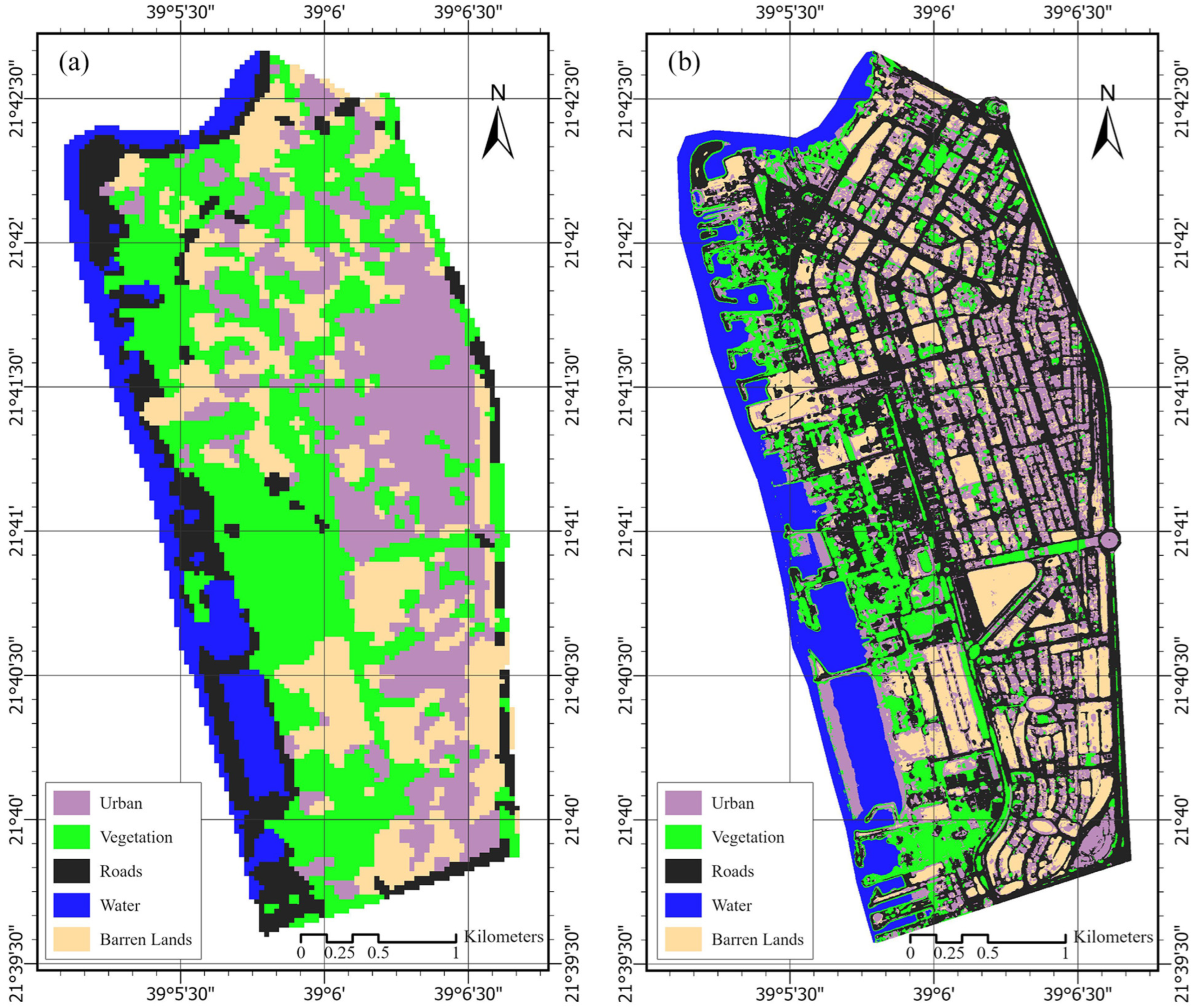
2.2.1. LULC Classification
2.2.2. LST Retrieval Using Landsat 8 Imagery
2.2.3. Measuring the Actual Temperature in the Field
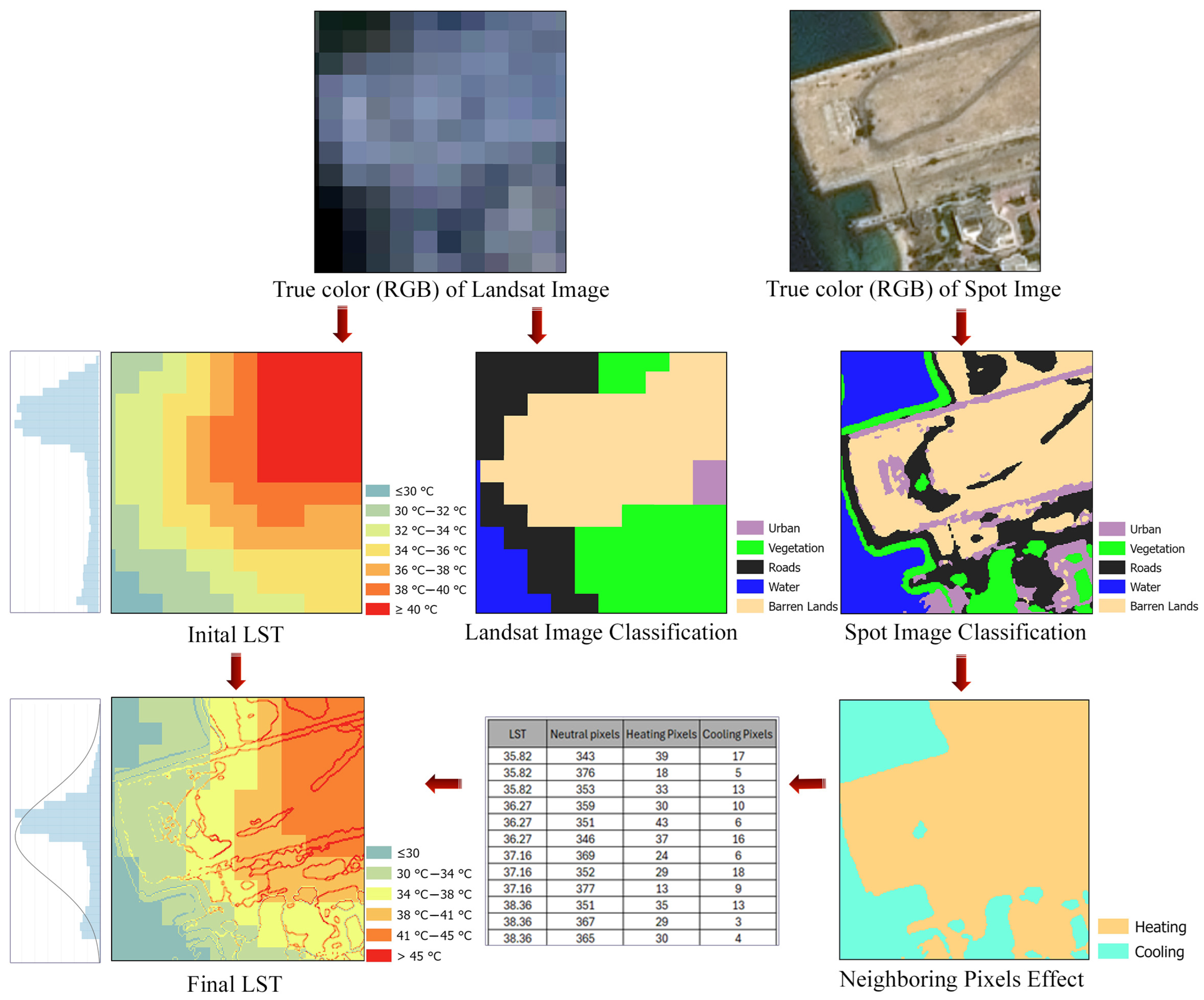
2.2.4. Temperature Correction Model
- (1)
- Each Spot-classified image pixel is assigned an initial temperature based on the closest homogeneous region of its classification category.
- (2)
- Influence parameters for each pixel based on the neighborhood analysis are assigned.
- (3)
- The average temperature for each Spot region covering a Landsat pixel is calculated, considering the influence coefficients α and β.
- (4)
- The best values for α and β are determined using the corrected Landsat temperature image and a machine learning model.
- (5)
- The actual temperature for each Spot image pixel is calculated.
3. Results
3.1. Classification of Images and Accuracy Assessment
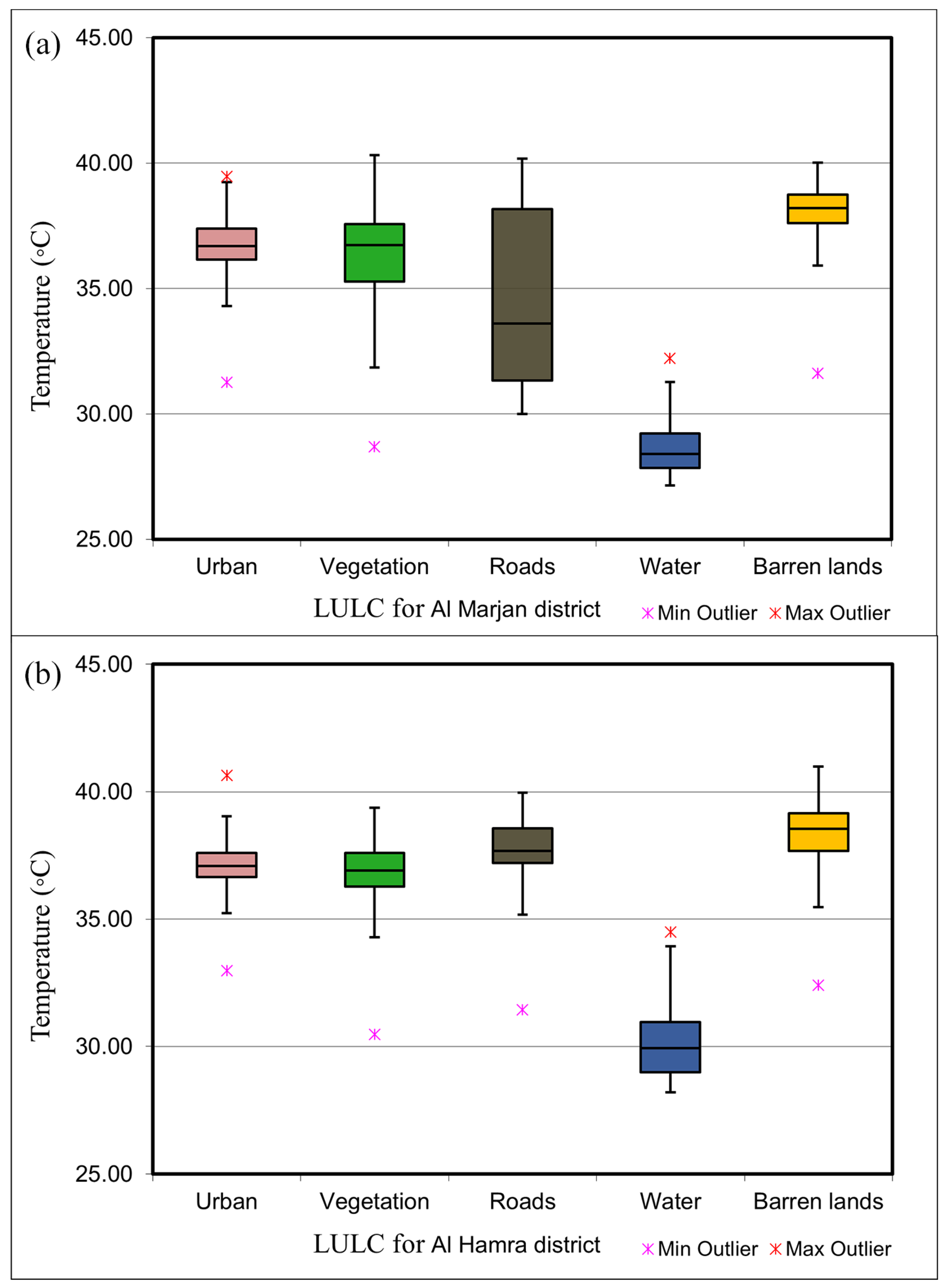
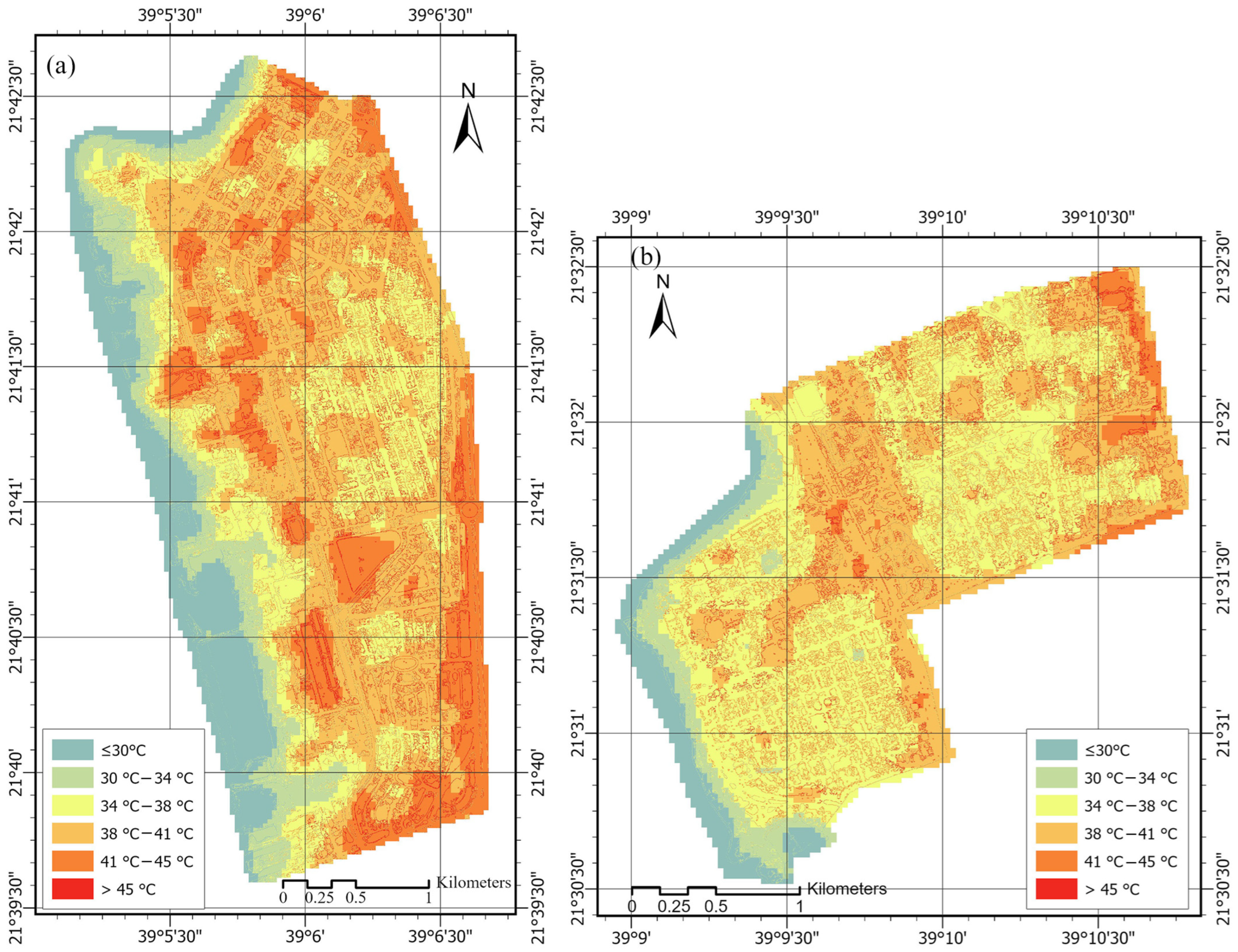
3.2. LST Spatial Distribution
3.3. LST Correction
3.3.1. Calculating the Cooling and Heating Coefficients
3.3.2. Neighboring Pixels Effect on LST
4. Discussion
5. Conclusions
Funding
Institutional Review Board Statement
Informed Consent Statement
Data Availability Statement
Acknowledgments
Conflicts of Interest
References
- Dash, P.; Göttsche, F.-M.; Olesen, F.-S.; Fischer, H. Land Surface Temperature and Emissivity Estimation from Passive Sensor Data: Theory and Practice-Current Trends. Int. J. Remote Sens. 2002, 23, 2563–2594. [Google Scholar] [CrossRef]
- Li, Z.-L.; Tang, B.-H.; Wu, H.; Ren, H.; Yan, G.; Wan, Z.; Trigo, I.F.; Sobrino, J.A. Satellite-Derived Land Surface Temperature: Current Status and Perspectives. Remote Sens. Environ. 2013, 131, 14–37. [Google Scholar] [CrossRef]
- Friedl, M.; Strahler, A. A Kernel-Driven Model of Effective Directional Emissivity for Non-Isothermal Surfaces. Prog. Nat. Sci. 2002, 12, 603–607. [Google Scholar]
- Vancutsem, C.; Ceccato, P.; Dinku, T.; Connor, S.J. Evaluation of MODIS Land Surface Temperature Data to Estimate Air Temperature in Different Ecosystems over Africa. Remote Sens. Environ. 2010, 114, 449–465. [Google Scholar] [CrossRef]
- Xu, T.; Guo, Z.; Xia, Y.; Ferreira, V.G.; Liu, S.; Wang, K.; Yao, Y.; Zhang, X.; Zhao, C. Evaluation of Twelve Evapotranspiration Products from Machine Learning, Remote Sensing and Land Surface Models over Conterminous United States. J. Hydrol. 2019, 578, 124105. [Google Scholar] [CrossRef]
- Xu, T.; He, X.; Bateni, S.M.; Auligne, T.; Liu, S.; Xu, Z.; Zhou, J.; Mao, K. Mapping Regional Turbulent Heat Fluxes via Variational Assimilation of Land Surface Temperature Data from Polar Orbiting Satellites. Remote Sens. Environ. 2019, 221, 444–461. [Google Scholar] [CrossRef]
- Tajfar, E.; Bateni, S.M.; Lakshmi, V.; Ek, M. Estimation of Surface Heat Fluxes via Variational Assimilation of Land Surface Temperature, Air Temperature and Specific Humidity into a Coupled Land Surface-Atmospheric Boundary Layer Model. J. Hydrol. 2020, 583, 124577. [Google Scholar] [CrossRef]
- Menon, S.; Akbari, H.; Mahanama, S.; Sednev, I.; Levinson, R. Radiative Forcing and Temperature Response to Changes in Urban Albedos and Associated CO2 Offsets. Environ. Res. Lett. 2010, 5, 014005. [Google Scholar] [CrossRef]
- Fu, P.; Weng, Q. A Time Series Analysis of Urbanization Induced Land Use and Land Cover Change and Its Impact on Land Surface Temperature with Landsat Imagery. Remote Sens. Environ. 2016, 175, 205–214. [Google Scholar] [CrossRef]
- Peng, J.; Ma, J.; Liu, Q.; Liu, Y.; Hu, Y.; Li, Y.; Yue, Y. Spatial-Temporal Change of Land Surface Temperature across 285 Cities in China: An Urban-Rural Contrast Perspective. Sci. Total Environ. 2018, 635, 487–497. [Google Scholar] [CrossRef]
- Masoudi, M.; Tan, P.Y. Multi-Year Comparison of the Effects of Spatial Pattern of Urban Green Spaces on Urban Land Surface Temperature. Landsc. Urban. Plan. 2019, 184, 44–58. [Google Scholar] [CrossRef]
- Miky, Y.H. Remote Sensing Analysis for Surface Urban Heat Island Detection over Jeddah, Saudi Arabia. Appl. Geomat. 2019, 11, 243–258. [Google Scholar] [CrossRef]
- Wu, C.; Li, J.; Wang, C.; Song, C.; Chen, Y.; Finka, M.; La Rosa, D. Understanding the Relationship between Urban Blue Infrastructure and Land Surface Temperature. Sci. Total Environ. 2019, 694, 133742. [Google Scholar] [CrossRef] [PubMed]
- Alexander, C. Normalised Difference Spectral Indices and Urban Land Cover as Indicators of Land Surface Temperature (LST). Int. J. Appl. Earth Obs. Geoinf. 2020, 86, 102013. [Google Scholar] [CrossRef]
- Miky, Y.; Al Shouny, A.; Abdallah, A. Studying the Impact of Urban Management Strategies and Spatiotemporal Dynamics of LULC on Land Surface Temperature and SUHI Formation in Jeddah, Saudi Arabia. Sustainability 2023, 15, 15316. [Google Scholar] [CrossRef]
- Bechtel, B. A New Global Climatology of Annual Land Surface Temperature. Remote Sens. 2015, 7, 2850–2870. [Google Scholar] [CrossRef]
- Bright, R.M.; Davin, E.; O’Halloran, T.; Pongratz, J.; Zhao, K.; Cescatti, A. Local Temperature Response to Land Cover and Management Change Driven by Non-Radiative Processes. Nat. Clim. Chang. 2017, 7, 296–302. [Google Scholar] [CrossRef]
- Tran, D.X.; Pla, F.; Latorre-Carmona, P.; Myint, S.W.; Caetano, M.; Kieu, H.V. Characterizing the Relationship between Land Use Land Cover Change and Land Surface Temperature. ISPRS J. Photogramm. Remote Sens. 2017, 124, 119–132. [Google Scholar] [CrossRef]
- Cai, M.; Ren, C.; Xu, Y.; Lau, K.K.-L.; Wang, R. Investigating the Relationship between Local Climate Zone and Land Surface Temperature Using an Improved WUDAPT Methodology—A Case Study of Yangtze River Delta, China. Urban. Clim. 2018, 24, 485–502. [Google Scholar] [CrossRef]
- Keenan, T.F.; Riley, W.J. Greening of the Land Surface in the World’s Cold Regions Consistent with Recent Warming. Nat. Clim. Chang. 2018, 8, 825–828. [Google Scholar] [CrossRef]
- Shen, Y.; Shen, H.; Cheng, Q.; Zhang, L. Generating Comparable and Fine-Scale Time Series of Summer Land Surface Temperature for Thermal Environment Monitoring. IEEE J. Sel. Top. Appl. Earth Obs. Remote Sens. 2021, 14, 2136–2147. [Google Scholar] [CrossRef]
- Colliander, A.; Fisher, J.B.; Halverson, G.; Merlin, O.; Misra, S.; Bindlish, R.; Jackson, T.J.; Yueh, S. Spatial Downscaling of SMAP Soil Moisture Using MODIS Land Surface Temperature and NDVI During SMAPVEX15. IEEE Geosci. Remote Sens. Lett. 2017, 14, 2107–2111. [Google Scholar] [CrossRef]
- Tang, R.; Li, Z.-L. An End-Member-Based Two-Source Approach for Estimating Land Surface Evapotranspiration From Remote Sensing Data. IEEE Trans. Geosci. Remote Sens. 2017, 55, 5818–5832. [Google Scholar] [CrossRef]
- Tang, R.; Li, Z. Estimating Daily Evapotranspiration From Remotely Sensed Instantaneous Observations With Simplified Derivations of a Theoretical Model. J. Geophys. Res. Atmos. 2017, 122, 10–177. [Google Scholar] [CrossRef]
- Gallego-Elvira, B.; Taylor, C.M.; Harris, P.P.; Ghent, D. Evaluation of Regional-Scale Soil Moisture-Surface Flux Dynamics in Earth System Models Based on Satellite Observations of Land Surface Temperature. Geophys. Res. Lett. 2019, 46, 5480–5488. [Google Scholar] [CrossRef]
- Zhao, W.; Wen, F.; Wang, Q.; Sanchez, N.; Piles, M. Seamless Downscaling of the ESA CCI Soil Moisture Data at the Daily Scale with MODIS Land Products. J. Hydrol. 2021, 603, 126930. [Google Scholar] [CrossRef]
- Lenschow, D.H.; Dutton, J.A. Surface Temperature Variations Measured from an Airplane over Several Surface Types. J. Appl. Meteorol. 1964, 3, 65–69. [Google Scholar] [CrossRef]
- Price, J.C. Land Surface Temperature Measurements from the Split Window Channels of the NOAA 7 Advanced Very High Resolution Radiometer. J. Geophys. Res. Atmos. 1984, 89, 7231–7237. [Google Scholar] [CrossRef]
- Ottlé, C.; Vidal-Madjar, D. Estimation of Land Surface Temperature with NOAA9 Data. Remote Sens. Environ. 1992, 40, 27–41. [Google Scholar] [CrossRef]
- Li, Z.-L.; Becker, F. Feasibility of Land Surface Temperature and Emissivity Determination from AVHRR Data. Remote Sens. Environ. 1993, 43, 67–85. [Google Scholar] [CrossRef]
- Sobrino, J.A.; Li, Z.-L.; Stoll, M.P.; Becker, F. Multi-Channel and Multi-Angle Algorithms for Estimating Sea and Land Surface Temperature with ATSR Data. Int. J. Remote Sens. 1996, 17, 2089–2114. [Google Scholar] [CrossRef]
- Wan, Z.; Dozier, J. A Generalized Split-Window Algorithm for Retrieving Land-Surface Temperature from Space. IEEE Trans. Geosci. Remote Sens. 1996, 34, 892–905. [Google Scholar] [CrossRef]
- Qin, Z.; Dall’Olmo, G.; Karnieli, A.; Berliner, P. Derivation of Split Window Algorithm and Its Sensitivity Analysis for Retrieving Land Surface Temperature from NOAA-advanced Very High Resolution Radiometer Data. J. Geophys. Res. Atmos. 2001, 106, 22655–22670. [Google Scholar] [CrossRef]
- Sun, D.; Pinker, R.T. Estimation of Land Surface Temperature from a Geostationary Operational Environmental Satellite (GOES-8). J. Geophys. Res. Atmos. 2003, 108, 4326. [Google Scholar] [CrossRef]
- Jiménez-Muñoz, J.C.; Sobrino, J.A. A Generalized Single-channel Method for Retrieving Land Surface Temperature from Remote Sensing Data. J. Geophys. Res. Atmos. 2003, 108, 4688. [Google Scholar] [CrossRef]
- Tang, B.; Bi, Y.; Li, Z.-L.; Xia, J. Generalized Split-Window Algorithm for Estimate of Land Surface Temperature from Chinese Geostationary FengYun Meteorological Satellite (FY-2C) Data. Sensors 2008, 8, 933–951. [Google Scholar] [CrossRef] [PubMed]
- Rozenstein, O.; Qin, Z.; Derimian, Y.; Karnieli, A. Derivation of Land Surface Temperature for Landsat-8 TIRS Using a Split Window Algorithm. Sensors 2014, 14, 5768–5780. [Google Scholar] [CrossRef]
- Li, Z.; Wu, H.; Duan, S.; Zhao, W.; Ren, H.; Liu, X.; Leng, P.; Tang, R.; Ye, X.; Zhu, J.; et al. Satellite Remote Sensing of Global Land Surface Temperature: Definition, Methods, Products, and Applications. Rev. Geophys. 2023, 61, 1–77. [Google Scholar] [CrossRef]
- Reiners, P.; Sobrino, J.; Kuenzer, C. Satellite-Derived Land Surface Temperature Dynamics in the Context of Global Change—A Review. Remote Sens. 2023, 15, 1857. [Google Scholar] [CrossRef]
- Price, J.C. Estimating Surface Temperatures from Satellite Thermal Infrared Data—A Simple Formulation for the Atmospheric Effect. Remote Sens. Environ. 1983, 13, 353–361. [Google Scholar] [CrossRef]
- Qin, Z.; Karnieli, A.; Berliner, P. A Mono-Window Algorithm for Retrieving Land Surface Temperature from Landsat TM Data and Its Application to the Israel-Egypt Border Region. Int. J. Remote Sens. 2001, 22, 3719–3746. [Google Scholar] [CrossRef]
- McMillin, L.M. Estimation of Sea Surface Temperatures from Two Infrared Window Measurements with Different Absorption. J. Geophys. Res. 1975, 80, 5113–5117. [Google Scholar] [CrossRef]
- Becker, F.; Li, Z.-L. Towards a Local Split Window Method over Land Surfaces. Int. J. Remote Sens. 1990, 11, 369–393. [Google Scholar] [CrossRef]
- Gillespie, A.; Rokugawa, S.; Matsunaga, T.; Cothern, J.S.; Hook, S.; Kahle, A.B. A Temperature and Emissivity Separation Algorithm for Advanced Spaceborne Thermal Emission and Reflection Radiometer (ASTER) Images. IEEE Trans. Geosci. Remote Sens. 1998, 36, 1113–1126. [Google Scholar] [CrossRef]
- Tonooka, H. An Atmospheric Correction Algorithm for Thermal Infrared Multispectral Data over Land-a Water-Vapor Scaling Method. IEEE Trans. Geosci. Remote Sens. 2001, 39, 682–692. [Google Scholar] [CrossRef]
- Wan, Z.; Li, Z.-L. A Physics-Based Algorithm for Retrieving Land-Surface Emissivity and Temperature from EOS/MODIS Data. IEEE Trans. Geosci. Remote Sens. 1997, 35, 980–996. [Google Scholar] [CrossRef]
- Zhao, Z.-Q.; He, B.-J.; Li, L.-G.; Wang, H.-B.; Darko, A. Profile and Concentric Zonal Analysis of Relationships between Land Use/Land Cover and Land Surface Temperature: Case Study of Shenyang, China. Energy Build. 2017, 155, 282–295. [Google Scholar] [CrossRef]
- He, B.-J.; Zhao, Z.-Q.; Shen, L.-D.; Wang, H.-B.; Li, L.-G. An Approach to Examining Performances of Cool/Hot Sources in Mitigating/Enhancing Land Surface Temperature under Different Temperature Backgrounds Based on Landsat 8 Image. Sustain. Cities Soc. 2019, 44, 416–427. [Google Scholar] [CrossRef]
- Li, J.; Song, C.; Cao, L.; Zhu, F.; Meng, X.; Wu, J. Impacts of Landscape Structure on Surface Urban Heat Islands: A Case Study of Shanghai, China. Remote Sens. Environ. 2011, 115, 3249–3263. [Google Scholar] [CrossRef]
- Chen, A.; Yao, L.; Sun, R.; Chen, L. How Many Metrics Are Required to Identify the Effects of the Landscape Pattern on Land Surface Temperature? Ecol. Indic. 2014, 45, 424–433. [Google Scholar] [CrossRef]
- Saudi Arabia Population Statistics 2023. Available online: https://www.stats.gov.sa/en (accessed on 10 October 2024).
- Elfadaly, A.; Shams eldein, A.; Lasaponara, R. Cultural Heritage Management Using Remote Sensing Data and GIS Techniques around the Archaeological Area of Ancient Jeddah in Jeddah City, Saudi Arabia. Sustainability 2019, 12, 240. [Google Scholar] [CrossRef]
- Google Earth Engine Platform. Available online: https://earthengine.google.com/platform/ (accessed on 10 October 2024).
- United States Geological Survey (USGS). Landsat 8 (L8) Data Users Handbook. Available online: https://www.usgs.gov/landsat-missions/landsat-8-data-users-handbook (accessed on 10 October 2024).
- Bokaie, M.; Zarkesh, M.K.; Arasteh, P.D.; Hosseini, A. Assessment of Urban Heat Island Based on the Relationship between Land Surface Temperature and Land Use/Land Cover in Tehran. Sustain. Cities Soc. 2016, 23, 94–104. [Google Scholar] [CrossRef]
- El-Hattab, M.; Amany, S.M.; Lamia, G.E. Monitoring and Assessment of Urban Heat Islands over the Southern Region of Cairo Governorate, Egypt. Egypt. J. Remote Sens. Space Sci. 2018, 21, 311–323. [Google Scholar] [CrossRef]
- Shirani-bidabadi, N.; Nasrabadi, T.; Faryadi, S.; Larijani, A.; Shadman Roodposhti, M. Evaluating the Spatial Distribution and the Intensity of Urban Heat Island Using Remote Sensing, Case Study of Isfahan City in Iran. Sustain. Cities Soc. 2019, 45, 686–692. [Google Scholar] [CrossRef]
- Dissanayake, D.; Morimoto, T.; Ranagalage, M.; Murayama, Y. Land-Use/Land-Cover Changes and Their Impact on Surface Urban Heat Islands: Case Study of Kandy City, Sri Lanka. Climate 2019, 7, 99. [Google Scholar] [CrossRef]
- Simwanda, M.; Ranagalage, M.; Estoque, R.; Murayama, Y. Spatial Analysis of Surface Urban Heat Islands in Four Rapidly Growing African Cities. Remote Sens. 2019, 11, 1645. [Google Scholar] [CrossRef]
- Sultana, S.; Satyanarayana, A.N.V. Assessment of Urbanisation and Urban Heat Island Intensities Using Landsat Imageries during 2000–2018 over a Sub-Tropical Indian City. Sustain. Cities Soc. 2020, 52, 101846. [Google Scholar] [CrossRef]


| Image | Urban | Roads | Vegetation | Barren Lands | Water | ||||||
|---|---|---|---|---|---|---|---|---|---|---|---|
| Area (km2) | Area% | Area (km2) | Area% | Area (km2) | Area% | Area (km2) | Area% | Area (km2) | Area% | ||
| Al Marjan | Landsat | 2.586 | 24.98% | 1.185 | 11.45% | 3.479 | 33.61% | 2.131 | 20.59% | 0.970 | 09.37% |
| Spot | 2.153 | 20.72% | 3.922 | 37.75% | 1.536 | 14.79% | 1.561 | 15.02% | 1.218 | 11.73% | |
| Al Hamra | Landsat | 1.533 | 25.90% | 2.844 | 42.03% | 0.952 | 10.09% | 0.524 | 08.85% | 0.422 | 07.13% |
| Spot | 1.069 | 18.15% | 2.837 | 48.15% | 0.735 | 12.47% | 0.881 | 14.95% | 0.370 | 06.28% | |
| Classification | Overall Accuracy | Kappa Coefficient | |
|---|---|---|---|
| Al Marjan | Landsat | 74% | 0.791 |
| Spot | 93% | 0.882 | |
| Al Hamra | Landsat | 77% | 0.802 |
| Spot | 95% | 0.894 | |
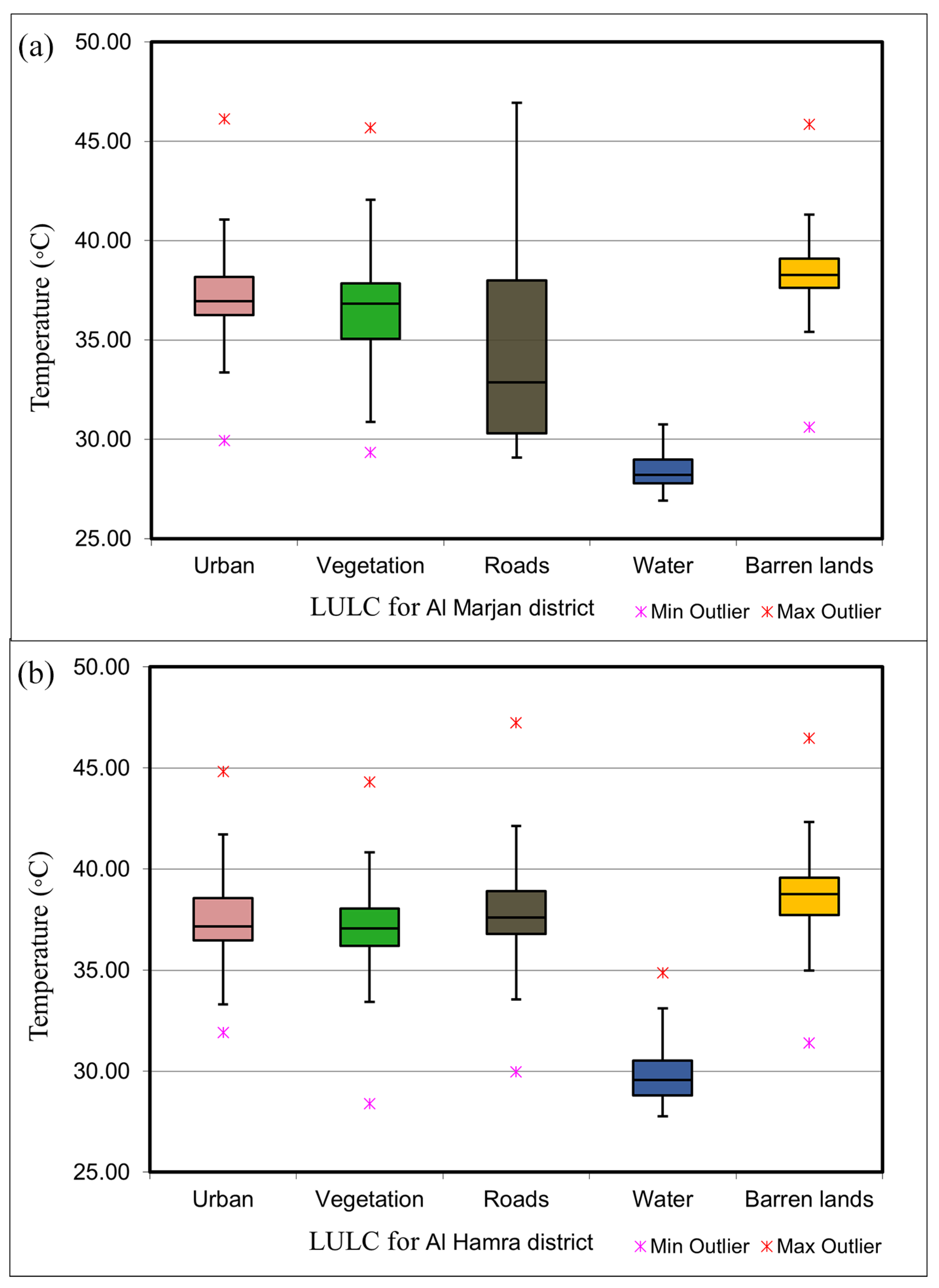
| Land Cover | Min. (°C) | Mean (°C) | Max. (°C) | Median (°C) | S.D. (°C) | |
|---|---|---|---|---|---|---|
| Urban | Al Marjan | 31.3 | 36.8 | 39.5 | 36.7 | 0.94 |
| Al Hamra | 33.0 | 37.2 | 40.6 | 37.1 | 0.88 | |
| Vegetation | Al Marjan | 28.7 | 36.2 | 40.3 | 36.6 | 2.02 |
| Al Hamra | 30.5 | 36.6 | 39.4 | 36.9 | 1.59 | |
| Roads | Al Marjan | 30.0 | 34.6 | 40.2 | 33.6 | 3.44 |
| Al Hamra | 31.4 | 37.8 | 40.0 | 37.7 | 1.10 | |
| Water | Al Marjan | 27.1 | 28.6 | 32.2 | 28.4 | 0.96 |
| Al Hamra | 28.2 | 30.1 | 34.5 | 29.9 | 1.29 | |
| Barren lands | Al Marjan | 31.6 | 38.1 | 40.0 | 38.2 | 0.95 |
| Al Hamra | 32.4 | 38.4 | 41.0 | 38.5 | 1.16 | |
| Land Cover | LST Range Estimated Image (°C) | LST Range Measured in the Field (°C) |
|---|---|---|
| Urban | 31.3–40.6 | 33.5–42.0 |
| Vegetation | 28.7–40.3 | 31.5–41.5 |
| Roads | 31.4–40.2 | 35.5–44.0 |
| Water | 27.1–34.5 | 29.0–32.0 |
| Barren lands | 31.6–41.0 | 36.0–44.5 |
| LST (°C) | Number of Spot Neutral Pixels/Landsat Pixel | Number of Spot Heating Pixels/Landsat Pixel | Number of Spot Cooling Pixels/Landsat Pixel |
|---|---|---|---|
| 36.27 | 359 | 29 | 10 |
| 36.27 | 351 | 43 | 6 |
| 37.16 | 352 | 29 | 19 |
| 38.36 | 351 | 36 | 13 |
| 39.43 | 358 | 25 | 17 |
| 39.43 | 346 | 37 | 17 |
| 40.42 | 371 | 16 | 13 |
| 41.15 | 357 | 29 | 14 |
| 41.71 | 345 | 40 | 15 |
| 42.26 | 352 | 30 | 18 |
| Urban | Vegetation | Roads | Water | Barren Lands | ||
|---|---|---|---|---|---|---|
| Al Marjan | Initial LST | 36.8 | 36.2 | 34.6 | 28.6 | 38.1 |
| Final LST | 38.2 | 37.4 | 38.0 | 29.0 | 39.1 | |
| Al Hamra | Initial LST | 37.2 | 36.6 | 37.8 | 30.1 | 38.4 |
| Final LST | 38.6 | 38.0 | 38.9 | 30.5 | 39.6 | |
Disclaimer/Publisher’s Note: The statements, opinions and data contained in all publications are solely those of the individual author(s) and contributor(s) and not of MDPI and/or the editor(s). MDPI and/or the editor(s) disclaim responsibility for any injury to people or property resulting from any ideas, methods, instructions or products referred to in the content. |
© 2024 by the author. Licensee MDPI, Basel, Switzerland. This article is an open access article distributed under the terms and conditions of the Creative Commons Attribution (CC BY) license (https://creativecommons.org/licenses/by/4.0/).
Share and Cite
Miky, Y. Studying the Impact of LULC Correspondence Between Landsat 8 and Spot 7 Data on Land Surface Temperature Estimation. Atmosphere 2024, 15, 1427. https://doi.org/10.3390/atmos15121427
Miky Y. Studying the Impact of LULC Correspondence Between Landsat 8 and Spot 7 Data on Land Surface Temperature Estimation. Atmosphere. 2024; 15(12):1427. https://doi.org/10.3390/atmos15121427
Chicago/Turabian StyleMiky, Yehia. 2024. "Studying the Impact of LULC Correspondence Between Landsat 8 and Spot 7 Data on Land Surface Temperature Estimation" Atmosphere 15, no. 12: 1427. https://doi.org/10.3390/atmos15121427
APA StyleMiky, Y. (2024). Studying the Impact of LULC Correspondence Between Landsat 8 and Spot 7 Data on Land Surface Temperature Estimation. Atmosphere, 15(12), 1427. https://doi.org/10.3390/atmos15121427