Future Low-Cost Urban Air Quality Monitoring Networks: Insights from the EU’s AirHeritage Project

Abstract

The last decade has seen a significant growth in the adoption of low-cost air quality monitoring systems (LCAQMSs), mostly driven by the need to overcome the spatial density limitations of traditional regulatory grade networks. However, urban air quality monitoring scenarios have proved extremely challenging for their operative deployment. In fact, these scenarios need pervasive, accurate, personalized monitoring solutions along with powerful data management technologies and targeted communications tools; otherwise, these scenarios can lead to a lack of stakeholder trust, awareness, and, consequently, environmental inequalities. The AirHeritage project, funded by the EU’s Urban Innovative Action (UIA) program, addressed these issues by integrating intelligent LCAQMSs with conventional monitoring systems and engaging the local community in multi-year measurement strategies. Its implementation allowed us to explore the benefits and limitations of citizen science approaches, the logistic and functional impacts of IoT infrastructures and calibration methodologies, and the integration of AI and geostatistical sensor fusion algorithms for mobile and opportunistic air quality measurements and reporting. Similar research or operative projects have been implemented in the recent past, often focusing on a limited set of the involved challenges. Unfortunately, detailed reports as well as recorded and/or cured data are often not publicly available, thus limiting the development of the field. This work openly reports on the lessons learned and experiences from the AirHeritage project, including device accuracy variance, field recording assessments, and high-resolution mapping outcomes, aiming to guide future implementations in similar contexts and support repeatability as well as further research by delivering an open datalake. By sharing these insights along with the gathered datalake, we aim to inform stakeholders, including researchers, citizens, public authorities, and agencies, about effective strategies for deploying and utilizing LCAQMSs to enhance air quality monitoring and public awareness on this challenging urban environment issue.

1. Introduction

Stakeholders’ awareness and concerns regarding urban air quality problems are continuously growing [1]. Air quality concerns are particularly perceived in densely populated urban areas where they can significantly and largely impact public health by exposing citizens to harmful pollutants [2,3]. It is well known, actually, that their inhalation can cause several effects, impacting respiratory organs (e.g., COPD, [4]), blood circulation (e.g., stroke), and the development of cancer [5]. In particular, short-term exposure to high NO₂ concentration levels is known to be a cause of severe asthma, while long-term exposure is usually associated with severe respiratory diseases [6]. Ozone has been well studied as an irritant of the upper respiratory pathways as a result of short-term exposure, while there is evidence of long-term effects in terms of accelerated decline in lung function and the progression of emphysema [7]. Inhaled particulate matter, depending on its size, can be found in several tissues where it accumulates and can be source of continuous oxidative stress, leading to development of ischemia [8] and cancer [9]. Hence, the increasing availability of accurate, factual knowledge about AQ concentration is a high-valued goal. It can give political decision makers and citizens the ability to act based on scientifically validated data with positive impacts on quality of life, public health, and further reducing environmental inequalities.

One of the first drivers of environmental inequalities is, actually, the scarcity of AQ information in localized areas of cities [10]. Obtaining pervasive data, however, is out of the operational envelope of the accurate but costly and bulky regulatory grade AQ analyzers, causing a number of research and innovation resources to focus on the development of low-cost air quality monitor devices. During recent years, a significant number of funded research and innovation projects have been devoted to the development of technological and methodological strategies for pervasive and accurate air quality monitoring (including OpenSense; Citi-Sense-MOB; EveryAware; Citi-Sense; “Schools for Better Air Quality” UNICEF Serbia pilot initiative, Breath London Network, Imperial County Community Air Quality Monitoring, etc. [11,12,13,14,15]), while commercial deployment, though in its early stage, is rapidly increasing. The main research and innovation question remains concerning how to design, develop, and test such innovative, hybrid technologies and monitoring networks, possibly increasing awareness and facilitating pervasive data gathering and exploitation. Secondarily, there are equally important questions regarded actual outcomes in terms of device accuracy, usability, and high-resolution mapping campaign outcomes. These complex projects face a number of difficult design choices, trying to accommodate technological and social science opportunities and limits with their general requirements and goals. They could target pervasive monitoring, citizen engagement, AQ information augmentation, traffic or heating regulation, etc., or any combination of these. Of course, the main target will inform and lead the choice of technical solutions regarding sensing units, acceptability, data management, accuracy, communication and quality management, human to machine interfaces, and software architectures. Unfortunately, commercial and innovation projects release limited, scattered, or incomplete information, while scientific reports appearing in the literature usually focus on a single aspect, lacking details on the other relevant ones. This make it quite difficult to obtain an overall and integrated comprehension of the challenges that should be tackled for the effective design, development, and deployment of LCAQMS networks. Moreover, the practice of open data is rather rare, thus limiting repeatability and comparison, and poses a decisive barrier for newcomers and experts in other fields to contribute effectively to solve the remaining technical and scientific challenges. Data scientists and modeling experts are particularly penalized by this behavior. This work aims to close this gap. By trying to address this goal, we describe the approaches implemented in the AirHeritage project regarding the overall technological infrastructure and associated methodologies. From the technical point of view, its main and/or novelty features are as follows:

• The development of a hybrid regulatory/LCAQMS network that integrates fixed and mobile opportunistic monitoring approaches;
• The integration of multiple (37) LCAQMS units from different producers;
• The implementation of multiseasonal repeated field calibration (using reference analyzers) and multiseasonal/multisite deployment;
• The use of edge computing for local and real-time concentration estimation and reporting through a smartphone app.
• The availability of user data (each user can download its own recorded raw and processed data while exploring its exposure data through advanced real-time and remote HCI using appropriate AQ index)
• Open data (comprising co-location and operative deployment data): anonymized data are available to researchers and users on Zenodo platform for the sake of repeatability, 10.5281/zenodo.13151960

A specific focus is given to the most challenging and resource-intensive issues of real-world deployments, including calibration, and to the impact of the design choices on the outcomes. The main findings in terms of accuracy, usability, and pollution events are presented.

The next sections focus on the description of general challenges along with the main components and solutions developed and/or adopted for the project implementation, respectively. These include the development of the AirHeritage version of the ENEA MONICA™ LCAQMS device (ENEA, Roma, Italy), their lab-based characterization, and the development of a full-blown IT infrastructure for AH network data gathering, processing, storage, and visualization. Furthermore, an efficient co-location strategy at the base of the adopted field calibration and validation approach is described. Eventually, the use of the gathered opportunistic measurements to generate ultra-high spatial resolution concentration maps is described, completing the technological and sensor data processing pipeline. Each of the steps are characterized by short and focused sentences highlighting the lessons learnt during the project implementation phase.

2. Main Challenges in Modern LCAQMS Deployments

Effective LCAQMS network deployment needs to tackle several technological and methodological challenges (see Figure 1). However, solutions may only become effective with respect to assigned or self-set objectives and relevant final users. The main objectives involve obtaining high accuracy data on some specific areas, which can be used to characterize localized pollution. On the contrary, one can reconstruct a high-resolution map using these data for data assimilation into a geostatistical or physically informed model.

In most cases, the measuring device will be conceived for a fixed deployment while the personal exposure assessment is extremely valuable and requires wearable or portable devices. If a target population and/or area of interest is large, both approaches will require significant resources for device station development/acquisition with respect to more focused goals.

Data accuracy requirements may differ with goals and targeted populations, ranging from remediation policy development to wide area coverage and citizen science community projects. The latter may be interested in anomaly detection for triggering more targeted studies while the former may need higher quality data for selecting appropriate actions based on validated data. When accuracy is the main concern, pinpointing the right sensing technology base is fundamental, though it may also conflict with available financial resources [16].

The data processing pipeline is fundamental to achieve the sought accuracy and the choice of calibration methodology is certainly at the core. Targeting concentration assessments, field calibration is the state of the art of LCAQMS calibration methodology, but this choice can rapidly generate logistic issues when the deployment node base is foreseen to exceed several tenths. This is becoming common; UNICEF Serbia, for example, has recently started a pilot project with more than 120 deployed units [14]. A growing trend can be observed for the number of devices currently involved in those projects, which aim to involve a large number of the citizens. They could be either citizen scientists cooperating with the monitoring activities or observers participating in reviewing the results in search for enhanced awareness and behavioral changes. The number of involved devices has a linear impact on the data inception stream size, which may prove challenging for management infrastructure dealing with the inception, processing, storage, and retrieval of data.

Depending on the goals, the measurement raw data stream may be entirely conveyed on centralized/cloud infrastructures or partially processed locally (edge computing) to transmit time averaged (e.g., on a minute, 15 min or hourly base) or processed value-added data (concentrations, thresholded alerts, combined AQ indices, etc.). Obtaining alerts, for example, could be extremely important for areas subjected to frequent fires as in the case of southern California, or in the case of nearby chemical processing industries.

As stated before, most of the projects focused on fixed AQ network development, but the development of portable and accurate AQ monitoring devices is equally important for obtaining personal exposure insights. A low cost is a very important feature when aiming for personal monitoring and is surely to be taken into account when targeting sustainable strategies for fixed installations in low-income countries where the highest concentrations of some pollutants can be recorded. Conversely, accuracy is again among the most sought-after feature when the increase in regulatory grade network spatial coverage is the main goal.

The acceptability and ease of use of sensor nodes will be paramount when citizen science is targeted [17]. Characteristics like weight and size could be decisive to guarantee that users abide by usage prescriptions (predetermined time and locations, opportunistic measurements, etc.). Easy access to anonymized or personally measured recorded data is of increasing interest both for citizen science and for administrative users. Eventually, preparing the citizens or policy makers to correctly grasp the meaning of measurements is a difficult task in itself, which requires adequate resources, as this is a matter of communicating AQ data through a universally understandable, accurately and concisely informed index without generating false expectations [18,19]. This, of course, depends on the cultural substrate, legal framework, and expectations. If legal framework accounting is based on the number of concentration threshold overshoots, then it could be easy to resort to this indicator. However, a common expectation is to use LCAQMS nodes to drive the local administration to act for remediation. Of course, this is most often a false expectation, since only regulatory grade monitoring device measurements are legally binding.

In this wide and complex framework, our group observed the peculiarity of the Italian and European scenario while selecting common worldwide requirements. Typically, small sized and densely populated urban settlements are mostly impacted by pollution generated by car traffic and household heating. Given the high density of historical features in city centers characterized by small spaces, the European legal framework and cost considerations prevented the development of pervasive air quality networks. As such, we recognized the role of citizen awareness while keeping the momentum towards accurate measurements. For this reason, we involved our partners in the development of the AirHeritage project. This has been an Urban Innovative Action project funded by EU under the ERDF framework to be implemented in Portici, a small city with a high population density, located 7 km south of Naples in southern Italy [20]. The main aim was increasing spatial and temporal density information about the most common air pollutants for administrative responses with a fixed dense LCAQMS network, while simultaneously involving citizen associations in the measurement process by deploying 30+ mobile devices, thus increasing citizens’ knowledge on personal exposure, further densifying the measurement process, and increasing citizens’ awareness. Aside from the measurement approach, a high-resolution AQ forecasting model, based on fluidynamic simulation, weather forecast data, and measurement data assimilation, developed by Terraria srl and Prof. Mazzoleni’s group from University of Naples, has been deployed. Several informative and preparatory campaigns with citizens and schools have been conducted with the support of Legambiente Campania, local associations, and the factual involvement of local administration authorities. This innovative, integrated, cooperative approach has strongly characterized the project ideation and development and ultimately guaranteed its technical and social success; however, we have to recognize that a thoroughly effective pollution mitigation policy needs a continued and sustained approach over time. This work actually focuses on sharing the lessons learnt on the technological side of the design and the operation of a pervasive and accurate measurement methodology culminating in the development of a hybrid network integrating fixed/mobile/regulatory grade analyzers.

3. The MONICA Low-Cost Air Quality Device

The MONICA device (shown in Figure 2 and Figure 3), a cornerstone of the AirHeritage Hierarchical network, exemplifies a robust and reliable approach to mobile and pervasive air quality monitoring. Its design prioritizes extended operational life, efficient data collection, and adaptability to both fixed and mobile monitoring scenarios. To facilitate widespread adoption, a compact form factor and lightweight design were paramount, while not sacrificing accuracy. These design choices were guided by three key considerations: sensor selection, optimized internal operations and power efficiency, and reliable data transmission.

3.1. Sensor Selection

The MONICA device leverages a combination of Alphasense™ electrochemical sensors (see [21]) and a Plantower particulate matter (PMS) sensor to provide comprehensive air quality monitoring. The electrochemical sensors, selected for their low-power consumption and accurate measurement of key pollutants, include carbon monoxide, nitrogen dioxide, and ozone.

Raw sensor data are processed by an Alphasense™ Analog Front End (AFE) component, converting current signals into voltages for subsequent acquisition. A dedicated temperature and humidity sensor is located in close proximity to the electrochemical sensors. These data are of paramount importance for the correction of measurement errors resulting from environmental fluctuations. The Plantower PMS sensor, with a resolution of 1 μg/m³ and an operating range of 0–500 μg/m³, offers precise measurements of PM_2.5 and PM₁₀ particulate matter [22]. An autonomous fan within this sensor guarantees optimal airflow and accurate particle detection.

3.2. Internal Operations and Power Efficiency

Data acquisition is handled by a low-power 32-bit STM32 microcontroller from STMicroelectronics™ (STMicroelectronics, Geneva, Switzerland). This choice balances processing power with minimal power consumption. The STM32 Nucleo™ board with a 12-bit ADC converts analog signals from the AFE into digital data for analysis. The ADC resolution and matching with the AFE output range ensures accurate measurements within typical air monitoring ranges (0–500 ppb for NO₂ and O₃, 0–12 ppm for CO). To shield the EC sensors from electromagnetic interference (EMI), part of the metal casing of the instrument acts as a Faraday cage. This is critical for gases such as NO₂ and O₃, which have poor air mixing and instability in partially open chambers. Fans address this by promoting gas–air mixing and mitigating instability through air injection. Their use is crucial, but their operation can impact power consumption. The MONICA instrument uses a dual approach: FW-switchable fixed speed fans for EC sensors with minimal airflow requirements to limit this problem, and autonomous fans for sensors requiring precise airflow control (PM sensor) to ensure overall optimum power consumption without compromising data accuracy.

A 3800 mAh Li-Po battery and a light and compact design provide the basis for extended mobility operation. This means at least 8 h of continuous air quality monitoring without recharging, a significant advantage for mobile applications.

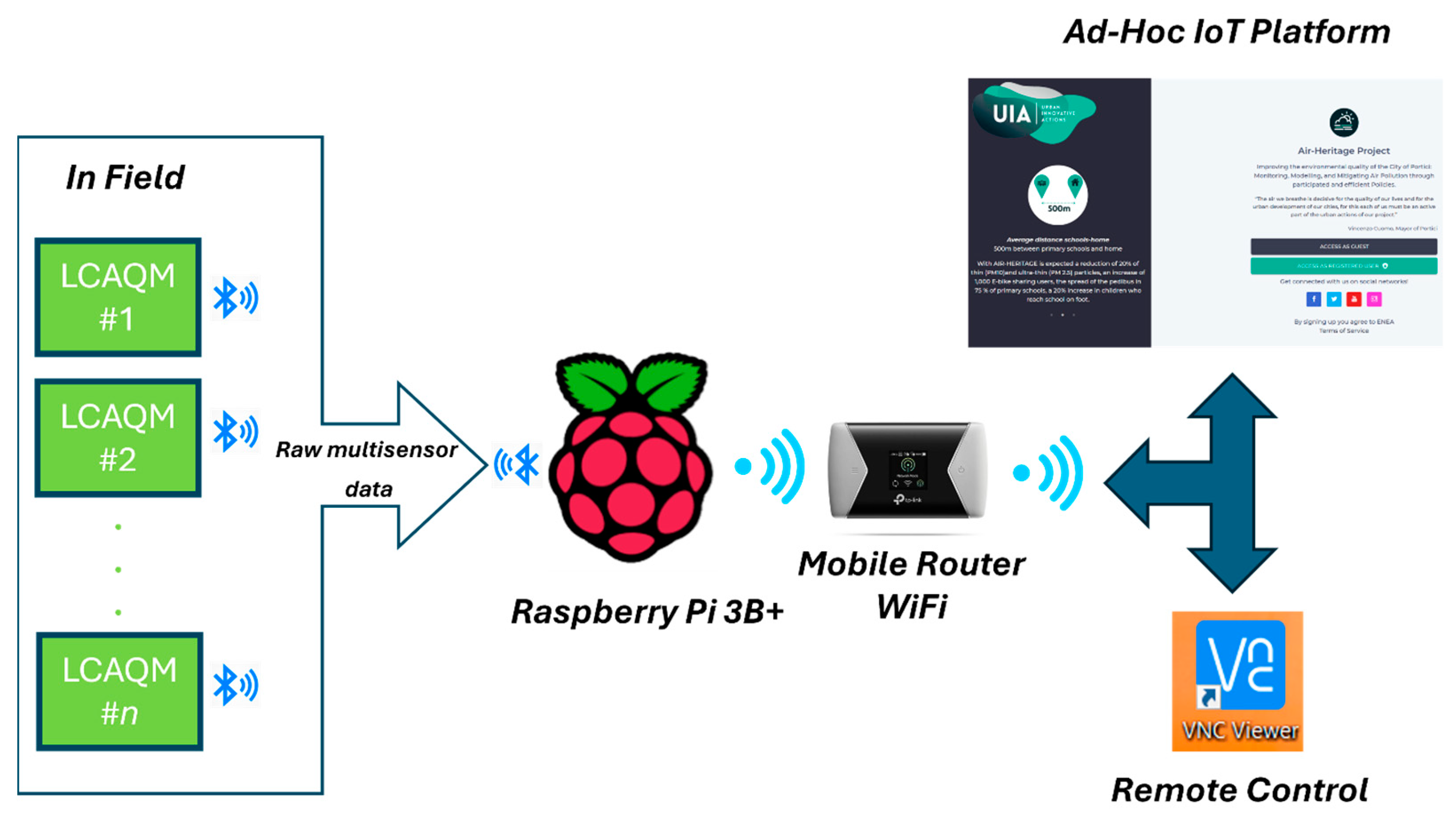
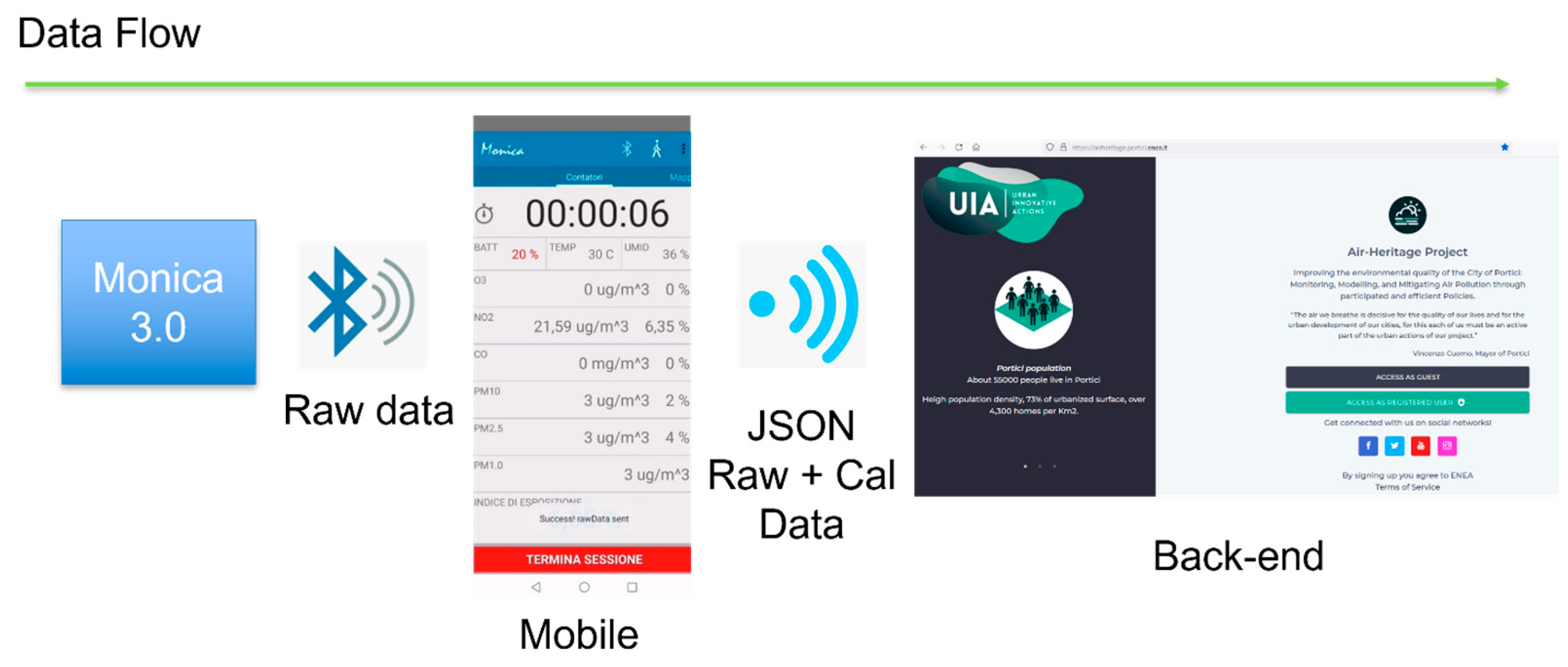
3.3. Communication and Data Transmission

The sensor node uses BLE technology to communicate with modern smartphones transmitting JSON payloads. This efficient wireless connection serves multiple purposes:

• Georeferencing: the smartphone’s GPS data can be used to geotag the collected air quality measurements, providing a critical spatial context for the collected data.
• Calibration implementation: calibration algorithms can be run on the smartphone to ensure the accuracy of sensor readings over time.
• Data transmission to the IoT back-end: the smartphone acts as a bridge, seamlessly transmitting the collected and processed air quality data to the central IoT back-end for further analysis and visualization.

The architectures and details of the user-side operation of sensor data transmission are explained in the following sections. A full component list of the MONICA device can be found in Supplementary Materials.

3.4. Considerations on the MONICA Design Outcomes and Recomendations

The MONICA system has been subjected to field testing in both stationery and mobile configurations. A deployment of 33 fixed-station units and 33 mobile units was undertaken. While a small percentage of malfunctions were observed, these were largely attributed to external factors or user errors. In fixed-station units, false contacts, battery degradation, and failed restarts due to prolonged interruptions in the external power supply accounted for 3%, 6%, and 12% of malfunctions, respectively. For mobile units, accidental damage from misuse was the leading cause of failure, comprising 18% of all incidents. The design of the MONICA device demonstrates the feasibility and effectiveness of creating a mobile air quality monitoring system that prioritizes low-power operation and efficient data collection. This approach offers several key benefits:

• Extended Mobile Operation: the low-power and comfortable-to-wear design choices ensure the MONICA device can work for extended periods without needing a recharge, making it ideal for mobile deployments in diverse environments.
• Accurate and Comprehensive Monitoring: the combination of various sensor technologies allows for the measurement of a broad range of air pollutants, providing a more holistic picture of air quality.
• Seamless Data Collection and Transmission: BLE connectivity with smartphones facilitates convenient data collection, georeferencing, calibration, and transmission to the central data storage and analysis platform.

Through the implementation of these strategies, the MONICA device enables more extensive and effective mobile air quality monitoring. By providing researchers and policy makers with a tool to collect air pollution data at a higher resolution, MONICA can contribute significantly to addressing urban pollution challenges.

4. Laboratory Characterization of MONICA Devices

4.1. Procedures for Laboratory Characterization and Calibration

Eleven MONICA™ devices were tested in a laboratory under controlled atmosphere conditions to verify their proper functioning and measure the performance of the sensors by comparing them with the specifications stated in the manufacturer’s calibration documents. The accuracy of the laboratory tests is ensured by the high quality of the instrumentation used and the laboratory’s twenty years of experience in studying solid-state gas sensors in controlled atmospheres. Specifically, for validating nitrogen dioxide concentration measurements, which is a very aggressive and difficult-to-control gas in enclosed environments, we used EPA-certified instrumentation (Teledyne T200 [23]). More than 50 tests were conducted, implementing measurement protocols to optimize the accuracy and precision of the tests and minimize measurement times. The equipment and measurement protocols are briefly described below.

A 15-L “Large Volume Test Chamber” (LVTC) has been installed in a state-of-the-art Gas Sensor Characterization System (GSCS). The GSCS consists of a stainless steel, air-tight test chamber enclosed in an adjustable thermal box. Within the LVTC, the air composition (humidity, chemical compound concentration) can be precisely controlled through an inlet of gas flux regulated by certified Mass Flow Controllers (MKS 1179 series) (MKS Instruments, Andover, MA, USA). The accuracy of the gas’s chemical composition is ensured by mixing gases from accredited bottles (Rivoira/Nippon Gases, Milano, Italy). Temperature and humidity are monitored with industrial sensors (LSI Pt100) (LSI LASTEM, Milano, Italy). The LVTC is capable of calibrating multiple sensor systems simultaneously.

The calibration method involves injecting a constant flow of the target gas, properly diluted to the maximum concentration (C₀) with humid synthetic air, into the inlet tube of the LVTC. The time-dependent concentration C(t) of the target gas is accurately predicted by the following exponential law, which generally describes the transition between two steady states of a physical parameter under a time-constant perturbation:

$$C\left(t\right)=C_0\left(1-e^{-{\displaystyle \frac{t}{\tau }}}\right)$$

(1)

A calibrated sensor can precisely estimate the characteristic time (τ). This parameter is proportional to the dead volume inside the chamber and must be appropriately corrected when multiple sensors are inside the chamber.

The calibration procedure consists of three steps: first, synthetic air is injected to establish the unperturbed state, recording the sensor output as a baseline; in the second step, the target gas, properly diluted in the gas carrier, is injected, and the adsorbing phase of the sensor response is recorded; finally, the third step involves washing the test chamber with a constant flow of synthetic air, recording the desorbing phase of the sensor output. This procedure allows for the verification of the sensor output behavior during the adsorbing and desorbing phases of the chemical compounds on the sensor surface. Sensing hysteresis or poisoning can be detected and measured.

With a gas flow rate of 1 L per minute, the τ of the LVTC is estimated to be 1100 s ± 50 s. This means that in 3 h, several sensors with a response time faster than 2 min can be calibrated with maximum precision from 0 to C₀.

For each tested device, the sensitivity to CO and NO₂ is verified, while for the ozone sensor, only the sensitivity versus NO₂ was tested.

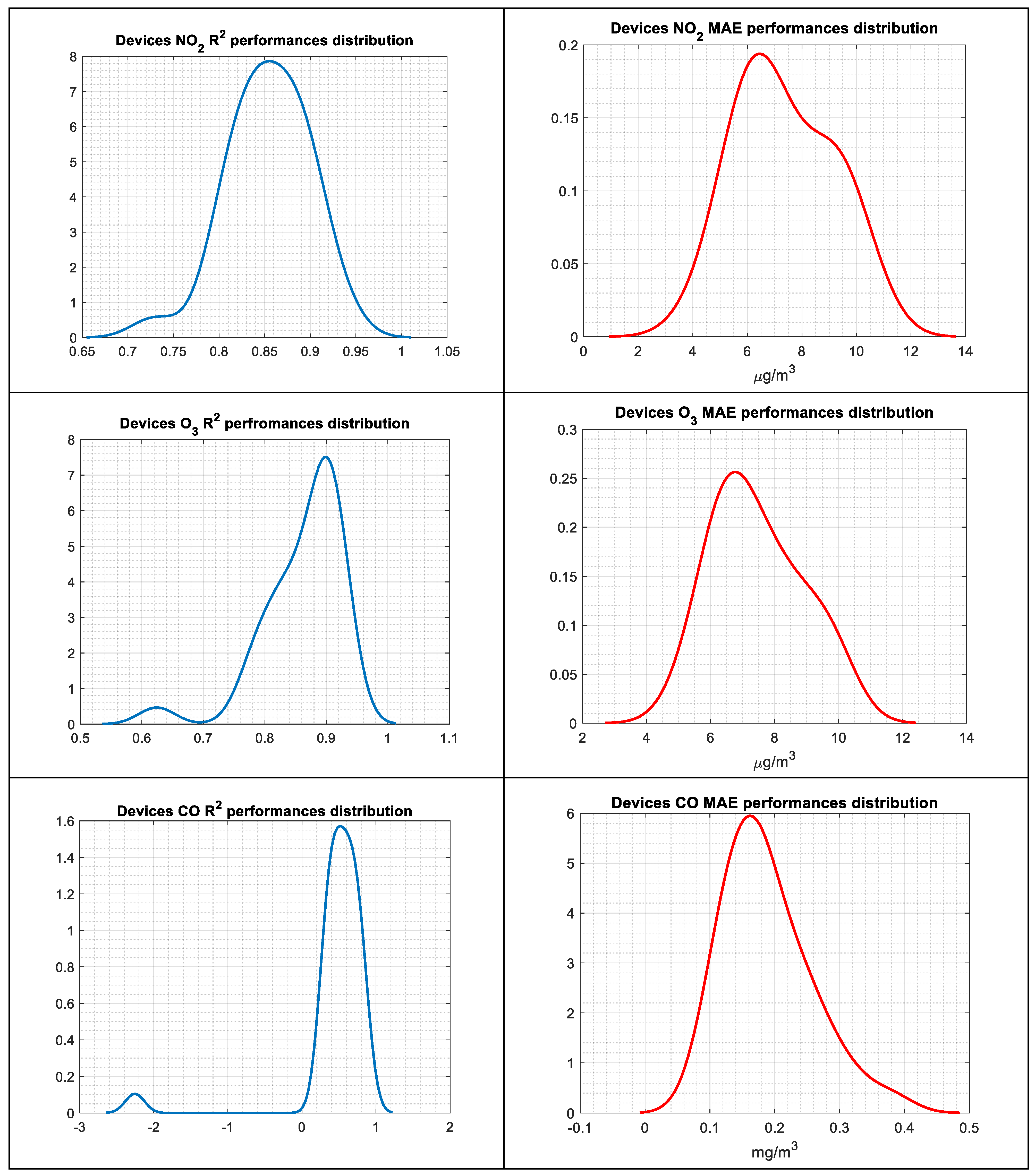
4.2. Results and Performance Improvement Suggestions

One of the most important aspects to control is the impact of sensor node case mounting on its performance. Worsened air mixing may impact on sensitivity and responsiveness. Furthermore, vendor-reported sensitivity and LOD characteristics should be checked to ensure the fulfillment of requirements when mounted. For these reasons, we strongly advise to check the node performance in laboratory controlled settings in order to capture the main issues that may affect the sensor when it is deployed in the field. Checking the interference impact is also very important for deciding about the calibration strategy and its parameters. Actually, the EC sensors installed on MONICA™ meet the expected performance standards and highlight the very well-known temperature dependance. More importantly, laboratory tests highlight the need to equip the devices with a fan in front of the NO₂ and NO₃ + O₃ sensors, having observed a loss of efficiency in measuring NO₂ in some cases. The fan speed was set to maximize the sensitivity of the sensors while minimizing power consumption.

5. Comprehensive Software Platform Development

5.1. Basic Software Requirements

The AirHeritage project handled diverse air quality data sources and aimed to offer several functionalities to citizens, which required the careful design of the software platform to meet all requirements. Two types of air quality sensors were deployed:

• ENEA MONICA sensors nodes operating at high sampling rates (about 3.5 s min sampling period set to 6 s);
• Commercial fixed stations by Digiteco srl [24], with data sampled every minute and transmitted every 15 min.

As above mentioned, the MONICA™ sensors were fully developed at the ENEA Portici research center. These devices are not equipped with wide area network connectivity and have no autonomous time clock reference. Consequently, data acquired from the devices must be sent via BLE to a device capable of transmitting the data to a remote server for centralized storage. The data must be augmented with a correct timestamp (in UTC format and synchronized with a time server). This device was either an Android smartphone using a dedicated app (for the mobility campaigns) or a custom sw equipped Raspberry Pi connected to Wi-Fi/cellular router. Data generated from MONICA™ is actually sent using BLE 5 to the WAN-enabled device in JSON format. Only raw, uncalibrated data are transmitted. This same format is used to send data using the HTTP protocol to the remote server. Raw data from MONICA devices should be augmented with calibrated data. In fact, only PM concentration values are directly available from the MONICA devices as expressed in µg/m³ (using Plantower sensor vendor calibration (Plantower, Nanchang, China)), and the calibration is performed on the edge device (i.e., an Android smartphone, although the same is possible on the Raspberry Pi).

Data from the fixed stations used in the project are sent via GPRS connectivity to an MQTT broker managed by the device supplier. The data are collected every minute and transmitted using the MQTT protocol every 15 min.

Data from the fixed stations comprise raw data as well as calibrated data. The initial calibration was provided by the device supplier using the default calibration from the sensor manufacturer. Later, after a co-location calibration, ENEA developed and compared multiple data-driven calibration methodologies, such as Multiple Linear Regression (MLR) and the Random Forest (RF) algorithm, significantly improving the provided measurements accuracy, with the RF algorithm expressing best short-term performances [25,26,27,28].

The platform needs to manage time series data from both sensor types, which requires handling large volumes of data and server traffic. Additional project requirements included the following:

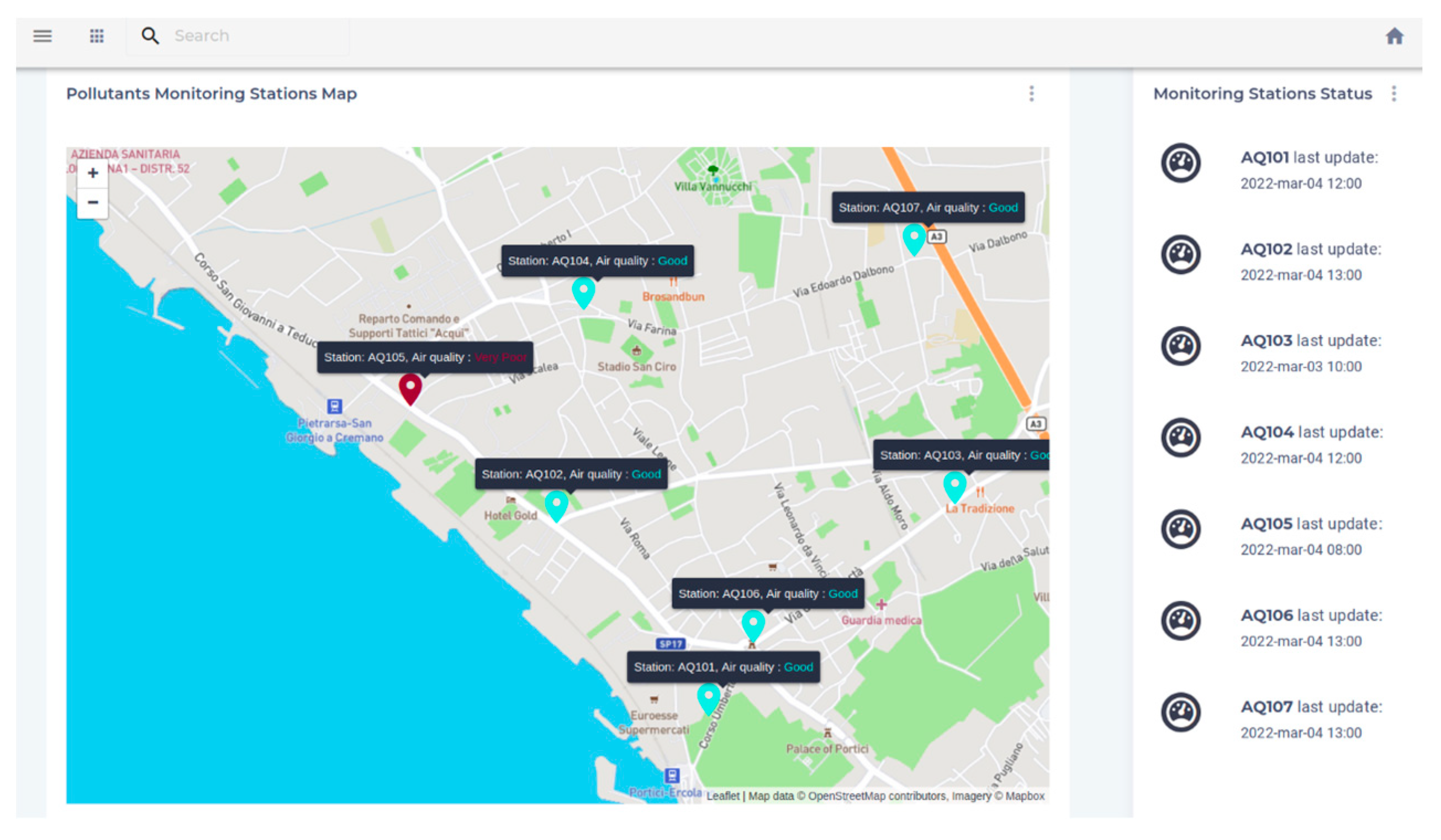
• An interactive map displaying the status of fixed stations, with the air quality index (AQI) updated every 15 min, based on MQTT data.
• The ability to download data in CSV format from fixed stations or specific sessions.
• Effective database management to maintain performance over time, even with multiple devices and extended MONICA sessions.
• Adherence to FAIR (Findability, Accessibility, Interoperability, and Reuse) principles for data access [29].
• Incorporation of best practices for service exposure and addressing cybersecurity concerns, including authentication and authorization.

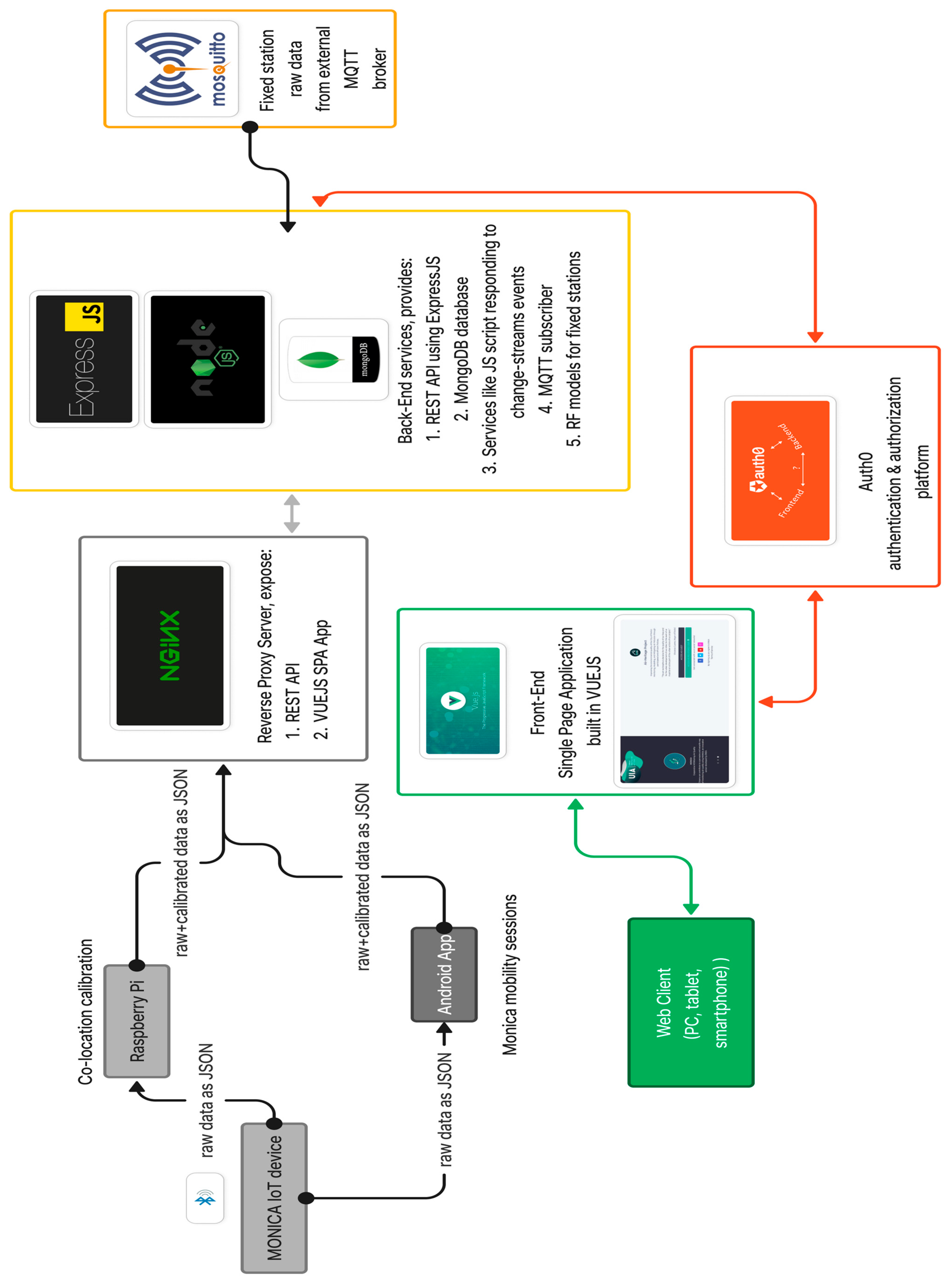
5.2. Architecture of the Developed Software Platform

The architecture, depicted in Figure 4, was developed after analyzing these requirements, ensuring robust performance, scalability, and security.

As shown in the figure, the designed software architecture for the AirHeritage project stores air quality data on a remote server using a REST (REpresentational State Transfer) API service [30]. This service handles CRUD (Create, Read, Update, Delete) operations via endpoints exposed by NGINX, a reverse proxy server [31]. Data are transmitted from the Android app or Raspberry Pi using the HTTP protocol in JSON format [32]. The REST API service was built using ExpressJS, a web framework based on NodeJS (https://nodejs.org/en) [33].

To secure certain REST API endpoints, especially those for CRUD operations, Oauth2 authorization was implemented [34]. Users need to sign up for a valid account to access these protected endpoints. For authentication and authorization, the project used Auth0, a third-party service that offers both free and paid tiers [35].

This approach made it possible to implement the following authentication mechanism:

• ▪ Social login using Facebook, Google, Twitter (now X);
• ▪ Account defined on Auth0 servers.

This allowed us to implement authentication and authorization in a simple and rapid way and support M2M (Machine to Machine) authentication for the Raspberry Pi devices [36].

Data from fixed stations were inserted into the database through a NodeJS application acting as an MQTT subscriber. Every 15 min, a proprietary binary message was sent by the MQTT broker, parsed, and saved into a MongoDB collection. Initially, data included both raw and calibrated pollutant values (e.g., CO, NO₂, PM₁₀), though the calibration was based solely on the sensor manufacturer’s specifications.

After a co-location calibration procedure, ENEA’s Random Forest (RF) model was deployed to improve data accuracy. This calibration process was implemented using JavaScript code on the server, running in NodeJS. MongoDB’s change-stream functionality was utilized to automatically trigger queries that extracted the inputs for the RF model, updating the collection with the new calibrated values whenever fresh data were inserted [37]. Similarly, another JavaScript script was used to compute the air quality index (AQI), updating it every 15 min.

These processes formed part of the back-end services hosted at the ENEA research center. The fron-tend was developed using Vue.js (version 2.x) and was chosen for its performance and flexibility in building web user interfaces. The project used additional JavaScript frameworks and libraries, including Vuetify for the user interface and VUE I18N for internationalization. Vue.js enabled the creation of a Single Page Application (SPA), a modern approach for web development [38]. Other alternatives considered included ReactJs and AngularJS.

Figures S1–S3 show the login process, starting from the website’s homepage (https://airheritage.portici.enea.it, accessed on 1 October 2024), where users can proceed as guests or sign in as registered users. As it can been, a careful approach has been taken from the graphical signage so as to maximize user acceptability. Auth0 was used for authentication and authorization, providing a consistent user interface for both Android and web browsers.

The front-end reported general information about the project and allowed users to view logged users’ registered MONICA sessions. It also displayed real-time data from fixed stations in terms of the AQI (Air Quality Index) on an interactive map (created using LeafletJS, https://leafletjs.com), with updates every 15 min [39,40].

Figure 5 and Figure 6 provide examples of the UI built for the project related to the two main features described earlier.

5.3. Data Management and Associated Monitoring Services

As already stated, data, mainly of the time series type, must be centrally stored. For this, a NoSQL-based solution was chosen: MongoDB Community Edition. This type of database, when using a proper schema for time series data, is well-suited for data coming from IoT devices. Moreover, horizontal scaling features like replica sets and sharding provide the necessary capabilities for a scalable and fault-tolerant solution, with authentication and authorization features available at the collection level. The following base collections were saved in MongoDB:

• MONICA sessions raw data;
• MONICA sessions calibrated data;
• Fixed stations raw data, factory calibrated data, and calibrated data using RF;
• Derived stats for all the above collections, populated automatically thanks to the change streams feature of MongoDB;
• AQI data derived from data at point 4, thanks to the change streams feature and a JS code (executed in NodeJS) to compute the AQI index (with color reference);
• Stats data by user for the citizen pricing campaign, computed using a JS app reacting to events generated by MongoDB change streams.

The choice to separate data into different collections was driven by the expected query patterns. The data schema was of the bucket type, with daily or session-based grouping in accordance with MongoDB best practices [41].

As described previously, the entire software solution is made up of many JS applications. Because both the front-end and the back-end use JS as their core, it constitutes what is known as a full-stack JS solution. These applications are monitored using PM₂, a commonly used process manager that monitors all the JS applications and restarts them in case of failures. To be notified in case of unhandled exceptions, Sentry (https://sentry.io/) [42] (a cloud service for remote error monitoring) was used for both the front-end app (VUE SPA https://vuejs.org/) and the back-end services. Similarly, Uptrends (a website availability monitoring service) was used to monitor the general availability of the web server. The software solution also sees the use of Failban [43] to monitor the NGINX logs and react automatically to handle anomalous traffic towards the server hosting the REST API and the SPA.

5.4. Software Integration and Utilization: Lessons Learned and Recommendations

The software solution/platform developed for AirHeritage was able to effectively handle the IoT device data from both MONICA and fixed stations, with some real-time functionalities thanks to the change-stream feature available in MongoDB for the replica-set configuration. Nonetheless, some elements could be improved, and although every solution has its pros and cons, the main findings from the experience gathered by the authors can be synthetically summarized below:

• The JSON serialization format could effectively be replaced by Protobuf for transmitting data from the Android/Raspberry Pi device to the cloud/remote server. This change could allow for more efficient data transmission, as Protobuf messages are much smaller in size compared to JSON (from 20% to 80% smaller than equivalent JSON messages) and this can reduce system latency [44].
• MQTT is definitely the preferred protocol for use at OSI layer 4 instead of HTTP [45].
• MongoDB was a valid and effective solution. However, current versions of MongoDB (especially starting from v.7 and later) implement TS collections that simplify code development while automatically handling IoT data in an efficient way. Sadly, this introduces some limitations, such as lack of support for the widely used change streams within the project, document size (4 MB compared to the generic MongoDB document limit of 16 MB), and more [46]. These limitations, hopefully, will be removed in future versions of MongoDB. For data coming from IoT devices, other solutions more tailored to TS data could be preferable, such as TimeScaleDB, InfluxDB, and QuestDB, to name a few.
• The REST API framework used within the project could be replaced with a solution based on a different language, such as Fiber for Go or FASTAPI in Python. However, a NodeJS-based solution is still, in the author’s opinion, a valid choice.
• To further improve scalability and fault tolerance, it could be useful to revisit the entire solution by employing Kubernetes (https://kubernetes.io/), with all services deployed using Docker (https://www.docker.com/) containers and adopting CI/CD practices [47].
• Although the FAIR principles were fulfilled as much as possible, adding an ontology to the data stored in MongoDB could certainly be a very attractive option [48].

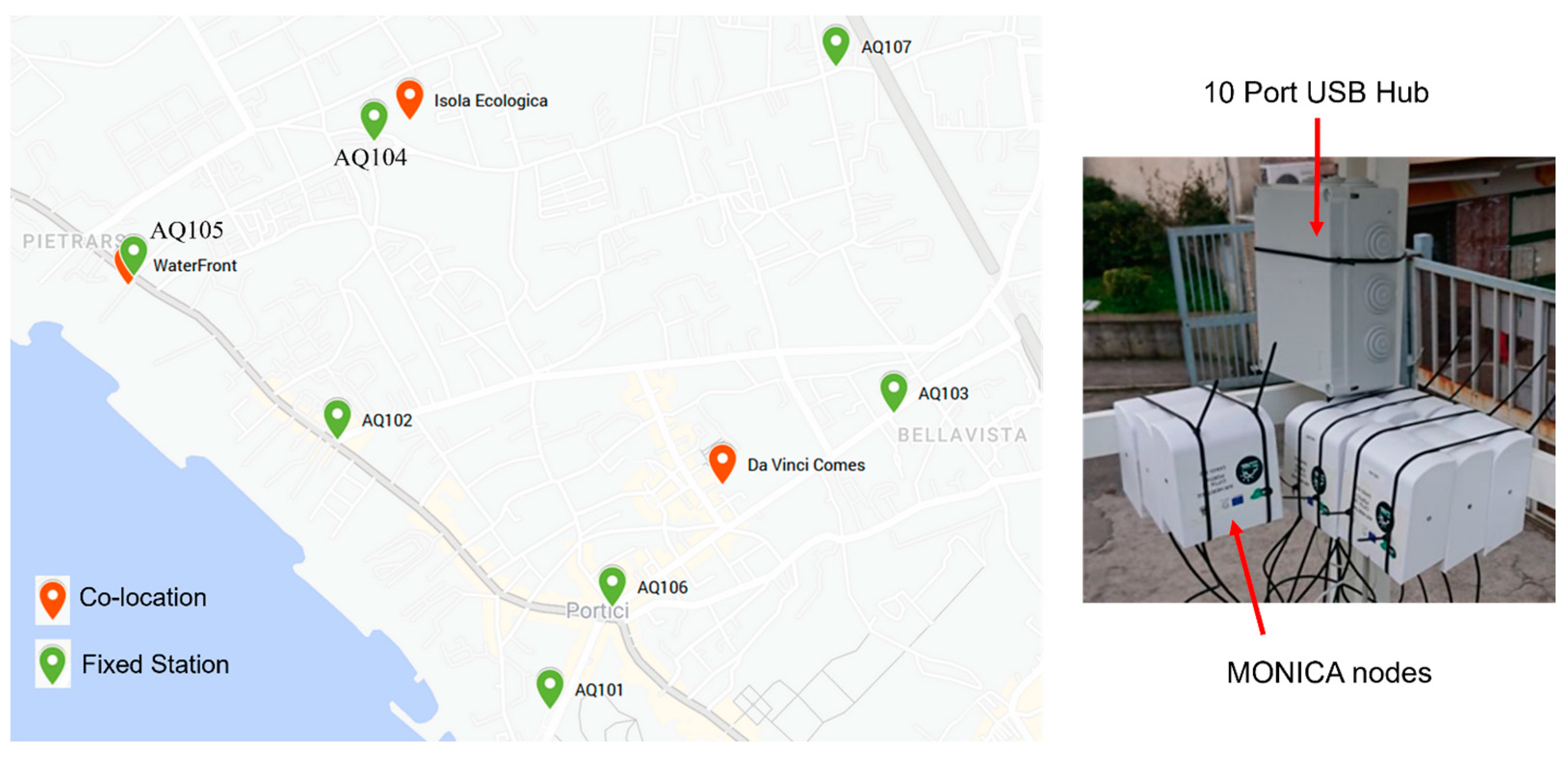
6. Effective Logistics Management for Co-Location Campaigns

6.1. General Co-Location Framework

The co-location of sensor nodes with a duly certified reference instrumentations is a prerequisite for progressing to the succeeding phase of node calibration by means of machine learning techniques [49]. It conveys significant information for characterizing sensor response in real-world scenarios. The aforementioned step of the AirHeritage project saw a fleet of thirty MONICA devices and the seven Commercial LCAQMS stations undergo three separate co-location periods in three distinct geographical areas of the Portici city. A mobile regulatory grade analyzer truck by ARPAC (Campania Environmental Protection Agency) was used as the reference station in all co-location campaigns. The characteristics of the reference air pollution analyzer parameters are reported in

Table 1. Instrumentation used on board the reference mobile laboratory.

Parameters	Technology	Type	Units
NOX	Chemiluminescence	Thermo Scientific Mod. 42i	µg/m3
CO	Non-dispersive infrared spectroscopy	Teledyne API Mod. T300	mg/m3
O3	Ultraviolet photometry	Teledyne API Mod. T400	µg/m3
PM10/PM2.5	Beta-ray attenuation	FAI Mod. SWAM 5a Dual Channel Monitor	µg/m3

.

The first co-location took place on 13 January 2021 at the “Portici WaterFront” site until 24 March 2021; the second co-location period start on 4 July 2021 at the “Isola Ecologica” site up to 4 October 2021, but with a long suspension period due to the temporary unavailability of the mobile laboratory. Further details are given in a metadata file associated with the resulting publicly available AirHeritage datalake (see Data Availability Statement section). Finally, the third co-location took place instead in “Scuola Da Vinci Comes” in Portici on 11 January 2022 until 13 April 2022.

The co-location campaigns occurred concurrently with the spread of COVID-19 and the introduction of legislative constraints in Italy due to the state of emergency. These restrictions effectively constrained the operations of the staff in the assembly and maintenance phases of the entire co-location campaigns.

6.2. Logistical Challenges and Implemented Solutions

Whether to co-locate all 30 units simultaneously or to divide them into groups for successive periods was one of the first concerns to be addressed. The latter option was selected for two fundamental reasons:

• The placement of the particulate matter instrumentation and other equipment of the institutional-grade mobile laboratory has resulted in a reduction of the available space on the roof of the vehicle, which has in turn constrained the capacity to accommodate the entire fleet of nodes.
• In order to prevent data loss and collisions between packets during transmission, a maximum of 10 nodes were connected to a single Raspberry Pi, which was employed as a concentrator node for aggregating and forwarding raw data from the nodes to the web server.

In order to guarantee an adequate quantity of data for the training phase, a minimum of three weeks of co-location is required for each individual batch.

Despite the MONICA device’s internal rechargeable battery, which is exerted for use in mobile sessions, when co-located, it is powered by a 10-Port USB hub and arranged in a fixed configuration. In this way, the co-located devices draw their power supply from the mobile laboratory’s main power distribution. Figure 7 illustrates the position of the co-location campaigns on the map and provides a detailed picture of the assembled devices.

The MONICA raw sensor data were captured and transmitted via Bluetooth Low Energy (BLE) to a Raspberry Pi Mod. 3B+ based datasink with Raspbian OS providing WAN connectivity services through a mobile router Wi-Fi TP-Link mod. M7650. Data acquisition is managed by a Python script running on the Raspberry Pi and managed through chron services. At the remote side, an ad hoc IoT back-end architecture relying on a contained NodeJS REST APIs server and MongoDB provides data inception, device management, storage, and data pre-processing (see Figure 8 and Section 5 for further details).

The integration of a Wi-Fi router into the IoT infrastructure design provides the additional benefit of enabling the remote control of data transmission. This is achieved by accessing the Raspberry Pi as a remote desktop with the RealVNC^® application (https://www.realvnc.com/en/). This enables the remote monitoring of data transmission, allowing for the continuous and automatic assessment of device functionality and the identification of instances of non-transmission. In the event that on-site verification is required, it could be easily scheduled.

The seven commercial station data streams were instead captured by the accompanying data transmission and MQTT-based brokerage system. Since they were powered by their photovoltaic panels, there was no need for exploiting external power sources, which provided an additional degree of freedom for optimally locating the stations as close as possible to the reference mobile station (see Figure 9).

It is crucial to acknowledge that any issues with the reference mobile vehicle power supply may impact on the entire network of the co-located devices. In the event of a power shortage, the internal battery of the Wi-Fi router will be discharged, thereby making remote access impossible.

During the second co-location campaign, which spanned from 4 July 2021 to 4 October 2021 at Isola Ecologica, the unavailability of the ARPAC mobile regulatory-grade truck, due to emergency relocation, necessitated the co-location of a number of nodes exceeding 10. This was performed in order to expedite the process in anticipation of future citizen science campaigns. In this particular situation, we elected to utilize two Raspberry Pi devices, apportioning half of the nodes to each individual Raspberry.

The latter highlights the importance and the difficulties related to the access to reference stations, which, in our case, was made possible thanks to the collaborative efforts of ARPAC. Direct access may also be impossible in several settings due to the unavailability of locally deployed reference stations, or the lack of resources needed to guarantee this access for research personnel to the regulatory grade stations. It is worth remembering that these, in turn, are designed and operated for different goals, and implement a strict regulatory framework to remain a source of authoritative data for the community.

6.3. Guidance for Future Co-Location Efforts

The IoT infrastructure-adopted solution has been demonstrated to be an effective and dependable approach for managing the data load of a subset of ten nodes. It is evident that the solution utilizing Raspberry Pi is a cost-effective and open-source option, particularly when combined with Python scripts.

Any effort should be made to allow for close co-location between all nodes and the reference analyzers. In case of a high number of LCAQMSs with significant dimensions, this may represent an issue, but accurate co-location planning after a site inspection may allow for an optimal trade off.

The decision to divide the fleet into three batches per co-location was largely a practical need, in our case. However, the management of a limited number of devices has proven to be an effective approach. This method allows for the periodic remote monitoring of node transmission status, which is a valuable tool for maintaining operational efficiency. Currently, this activity is performed manually and on a periodic basis. It is recommended that this process be automated in the future by developing a series of Python scripts that monitor the data transmission status and send an alert in the event of a prolonged lack of received data packets. Such an approach would facilitate timely interventions to resolve the problem, which could be of an electrical nature, a lack of power supply, or a variety of issues specific to the individual node. Furthermore, the management of a limited number of co-located nodes offers the additional benefit of facilitating maintenance activities.

Finally, we have attempted to exploit batching in order to assess the efficacy of novel calibration methodologies, including global calibration [50]. This methodology was developed with the specific objective of reducing co-location and calibration costs through the utilization of a virtual calibration model that incorporates the inherent variability of individual sensors. The findings indicate that co-locating a minimum of five nodes is sufficient to apply the virtual model to the remaining nodes for low-cost particulate matter sensors [51]. This approach is undoubtedly beneficial in the context of large-scale deployments. Further research is required to validate this approach on large deployments and to ascertain whether an extension to gas sensors is also feasible [52].

7. Calibration and Data Management

7.1. Low-Cost Sensor Calibration Methods

Most low-cost air quality sensors need a calibration law which translate their raw response values, usually encoded in electrical variables, in actual concentration data. Typical examples are MOX, which encode concentrations in resistivity, electrochemical sensors, which encode concentrations in electrical potentials, or Quartz Micro Balances (QMBs), the responses of which are encoded in frequency shifts [53]. Unfortunately, along with their undoubted advantages, they suffer from several operational issues which hinder the accuracy of calibrated values; these effects are particularly significant when deployed in the field. Among these, fabrication variance, which implies sensing unit characteristics variance, lack of stability, which makes these characteristics vary in time, environmental and non-target gases sensitivity, which makes their response vary with those factor intensities, are the most challenging. Their combined effect requires extensive and/or frequent recalibration actions in time or after relocation [54,55,56]. These considerations motivated us to proceed to develop a peculiar, though literature-based, calibration strategy, so to keep a balance between due efforts and accuracy with the latter as a priority. These, together with the device batch size, availability for actual deployments, and the need for reference data, constituted the operational and functional requirement envelope, which lead us to devise a seasonal recalibration protocol exploiting field calibration as the preferred and most accurate methodology [57]. Whenever available, co-location data provide the best reference data to achieve a data-driven calibration.

According to the plan described in the previous section and detailed in

Table 2. Co-location scheme of the mobile MONICA devices. The schema encompasses 3 periods in 3 different seasons and locations within the urban area of Portici (Naples). Colors are encoded for the initial batch partition during period 1 to highlight that batch partition changed in the different periods, so MONICA units could belong to different batches in different periods.

	Period 1 (2021)			Period 2 (2021)			Period 3 (2022)
#	Batch 1	Batch 2	Batch 3	Batch 1	Batch 2	Batch 3	Batch 1	Batch 2	Batch 3
	13 January 15:00 -> 5 February 12:00	5 February 12:00 -> 2 March 10:00	2 March 14:00 -> 24 March 10:00	4 July 00:00 -> 19 July 23:59	24 August 11:00 -> 14 September 8:40	14 September 10:15 -> 4 October 9:20	11 January 00:00 -> 2 February 23:59	9 February 00:00 -> 3 March 23:59	4 March 00:00 -> 13 April 23:59
1	337	325	324	332	327	324	324	327	325
2	339	326	330	340	330	325	326	328	356
3	344	327	334	349	331	326	329	349	353
4	345	329	335	350	333	329	334	355	350
5	349	331	343	353	334	343	339	347	335
6	353	332	350	356	335	_	338	345	330
7	355	333	351	360	337	_	344	331	332
8	356	340	352	362	339	_	361	333	341
9	360	341	362	_	341	_	_	337	351
10	361	364	363	_	344	_	_	343	_
11	_	_	_	_	345	_	_	_	_
12	_	_	_	_	351	_	_	_	_
13	_	_	_	_	355	_	_	_	_
14	_	_	_	_	363	_	_	_	_

, all fixed and mobile devices have been co-located with a reference analyzer for at least three weeks in three different seasons and locations within the city of Portici, the target city of the project. All raw data recorded during the co-location periods have been captured along with reference analyzer readings provided by the regulatory grade mobile monitoring station. Time reconciliated data series have been collected in the datalake comprising both fixed station and mobile station co-location data in order to support the selection, development, and testing of calibration algorithms (see Data Availability Statement section).

Once calibrated, the actual operative deployment occurred between consecutive calibration/co-location periods. The figures in the Supplementary Materials further show some of the operative deployment preparation phases including pre-charging for mobile devices, preparation to mobile device shipping, and the operative deployment of one of the fixed units.

Generally, AQ multisensory calibration algorithms use raw sensor data together with environmental variables, so as to correct their interferences and return concentration estimations as an output.

Formally, let $C=(C_1,C_2,\cdots ,C_n)$, which is the true concentration vector, and $X=\left(X_1,X_2,\cdots ,X_n\right)$, which is the input raw sensor readings matrix. The calibration stage aims to derive a function $f$, such that,

$$C=f\left(X\right)\mp \epsilon$$

(2)

with $\epsilon$ being the residual calibration error.

As we have seen before, raw gas sensor data encodes forcer information as analog voltages, frequency shifts, or IR spectras, whilst PM sensors either use particle count as raw data or provide a vendor-based calibrated output which can be used as “raw” input data. As we introduced above, response forcers may include target gas and other gaseous interferents as well as environmental interferents. The X vector may thus turn in a matrix, if including past records of the same variables and/or past target concentrations as stored in tapped delay lines (lagged values) for deriving dynamic and/or recurrent models, respectively. In our case, the input variable array X included raw data from the chosen electrochemical sensors (working and auxiliary electrode voltage) for target gas and interferents, plus environmental interferents. For NO₂, this is expressed as follows:

$$X=\left[\begin{array}{c}{WE}_{N{O}_2}\\ {AE}_{N{O}_2}\\ T\end{array}\right]$$

(3)

where ${WE}_{N{O}_2}$ (in mV) and ${AE}_{N{O}_2}$ (in mV) are the output of the working and auxiliary electrode, respectively, of the NO₂ sensor, and T is the temperature (in °C). In fact, the temperature is reported as one of the most significant interferents for electrochemical gas sensors. Actually, Alphasense itself advise to correct concentration estimations according to temperature values through specific application notes.

For CO gas concentration estimation, we used CO sensors, WE and AE voltages, plus temperature readings. Hence, X is instead given by the following:

$$X=\left[\begin{array}{c}{WE}_{CO}\\ {AE}_{CO}\\ T\end{array}\right]$$

(4)

Due to the well-known interference of NO₂ concentrations on the chosen sensors, O₃ concentration was estimated using sensor readings coming from NO₂ and O₃ sensors plus temperature readings:

$$X=\left[\begin{array}{c}\begin{array}{c}{WE}_{O_3}\\ {AE}_{O_3}\\ {WE}_{N{O}_2}\end{array}\\ {AE}_{N{O}_2}\\ T\end{array}\right]$$

(5)

Conversely, humidity served as the primary correction factor in the MLR model formulation for PM sensors. Hence, for the MONICA™ devices, we obtained the following:

$$X=\left[\begin{array}{c}{Conc}_{PM2.5/PM10}\\ RH\end{array}\right]$$

(6)

Note that the vendor-estimated size-fractioned concentration for the targeted pollutant was used as a raw sensor for the PMS7003 sensor calibration along with relative humidity readings.

According to the literature and our field deployment experience, 3 weeks of co-location data are sufficient to obtain optimal short-term accuracy performance [56,58]. Regarding the model choice, multilinear regression is actually providing a good balance between short-term precision and accuracy metrics while showing interesting generalization properties for mid-term deployments [59]. Comparatively, the Random Forest model, among non-linear machine learning approaches, is correctly referred to as providing the best accuracy for short-term deployment but fails to provide accurate concentration readings when operating outside the input ranges within which it has been trained. MLR has hence been chosen as a data-driven model for providing calibration for both gas and particulate sensors for mobile and fixed stations according to the following:

$$y=aX+b$$

(7)

where b is the intercept and a is the least square optimal coefficient.

In summary, to ensure the highest accuracy during long-term deployment, the AirHeritage project has implemented an edge computing, AI-based field calibration, using a data-driven derivation of an MLR model for each of the 30 mobile analyzers, with periodical (seasonal) recalibration. Short-term accuracy figure estimations for the MONICA devices, obtained during period 1, are reported in

Table 3. Cross-validated MLR performance metrics averaged for the 30 MONICA devices (2 consecutive weeks for the training length, 1 week for the test length, and 2 temporal stratifications over 3 weeks) during the first co-location period. Negative estimations are reverted to null concentrations. Bold characters emphasized median values while red highlights the best performance obtained for the specific indicator among all pollutants under consideration.

		Train	Test	MAE	R2	RMSE	NRMSE	MAPE
		#Hrs	#Hrs	µg/m3	N/A	µg/m3	µg/m3	N/A
O3	AVG	322.7	207.3	7.46	0.86	9.59	0.35	0.08
	STD	25.6	35.3	1.92	0.10	3.00	0.12	0.02
	MDN	330	203.5	6.99	0.88	9.32	0.33	0.08
NO2	AVG	322.7	207.3	7.92	0.83	10.32	0.41	0.08
	STD	25.62	35.4	2.41	0.08	3.10	0.09	0.02
	MDN	330	203.5	6.95	0.86	9.07	0.38	0.07
CO	AVG	322.7	207.3	190	0.33	260	0.74	0.12
	STD	25.62	35.4	80	1.02	0.12	0.34	0.04
	MDN	330	203.5	190	0.51	240	0.69	0.11
PM2.5	AVG	323.5	195.5	5.49	0.75	7.43	0.49	0.07
	STD	25.8	35.1	1.12	0.11	1.38	0.11	0.02
	MDN	323.5	195.5	5.13	0.75	7.32	0.50	0.08
PM10	AVG	321.9	206.7	13.07	0.42	20.84	0.75	0.10
	STD	25.4	34.8	4.83	0.19	12.94	0.12	0.03
	MDN	329.5	202.5	11.86	0.43	14.10	0.76	0.10

. Cross-validated MLR performance metrics averaged for the 30 MONICA devices (2 consecutive weeks for the training length, 1 week for the test length, and 2 temporal stratifications over 3 weeks) during the first co-location period. Negative estimations are reverted to null concentrations. It is important to stress the relevance of estimating performance using consecutive, temporally stratified, training and test sets, thus avoiding any data leaks and simulating real deployment conditions. In this case, we can thus obtain realistic performance index estimations. According to the literature, regulatory agencies activities in LCAQMS characterization, and finally, to the different national and international regulatory frameworks, the mean absolute error (MAE), mean absolute performance error (MAPE), and coefficient of determination (R²) appear among the most frequently used and shared performance indicators. We hence decided to use them to guarantee a quick but comprehensive assessment of the device performance. In terms of the coefficient of determination, depending on the pollutant species, we obtained values which span from 0.43 of PM₁₀ estimations to 0.88 for ozone concentration estimations. Low values obtained for PM₁₀ can be explained by the low sensitivity of the specific sensor to that particulate fraction size, as it is well-known that most of the low-cost particulate sensors are optically tuned to express maximum sensitivity to the PM_2.5 fraction. Lower performances expressed in the CO estimation can also be explained by the low concentrations recorded during the specific co-location period (see Figure 10 and Figure 11), which proved to be very challenging for the adopted sensor unit and for the reference analyzer. In fact, reference station hourly recordings highlight a mid to low pollution condition level when compared with respective (multi-)hourly or daily average thresholds set in the EU regulation framework. However, recorded PM_2.5 and NO₂ concentration can become of a certain concern when compared to recent WHO guidelines.

Due to inherent fabrication variance and to different training/test set periods, device performances express an interesting variance. However, the analysis of performance variance showed that in this short-term deployment, with the exception of short-term transients, we did not record performance extremes with all devices showing consistent performance ratings (see Table 3). Just as an example, R² ratings showed a minimum value of 0.72 and a maximum value of 0.93. Since the actual concentration range is a significant factor influencing performance, we also report that MAPE readings were comprised between a minimum of 4.4% and a maximum of 9.4%; in the latter case, the device kept an R² of 0.78. More comprehensively, Figure 12 and Figure 13 report the empirical distribution of the MAE and R² values over the 30 devices. These highlight the presence of a noticeable variance corresponding to the different performance obtained by the groups co-located in the three different batches of the 2021 winter period, again highlighting the relevance of actual co-location conditions (see Figure 14). In some cases (see CO figures), the distribution highlights a limited number of underperforming devices whose performances are explained by short-term transients occurring at sensors with the first switch on. Figure S7 a to e repots the results obtained in terms of the RMSE for all the relevant pollutants across the 30 MONICA devices.

Unfortunately, our multiseasonal recordings confirmed that ab initio field calibration long-term performances show a significant performance drop, which requires re-calibration at least on a seasonal basis, which we actually performed. As an example, R² figures for PM_2.5 dropped to an average 0.26, as we reported in [58].

We remind the reader that the calibration function was actually executed on a smartphone, enabling immediate and localized feedback to the user while they move across the city, which resulted in a strongly appreciated feature. In doing so, we decided to temporarily store calibration parameters in the Android app resource files, where they are retrieved at the start of each recording session. This allows for updates without needing to rewrite the device firmware and the need for stable connectivity, though it still urges users to download a new APP version at each campaign start, following the actual calibration parameter derivation phase. However, as cellular connectivity has reached operational maturity, allowing for stable connections almost everywhere, we chose, for the next version of the MONICA ecosystem, to provide an upgrade to store calibration parameters on centralized inception and storage facilities, eliminating the need for app updates. This will also make it easier to constantly upgrade calibration parameters if a remote calibration strategy will be in place.

7.2. Guidance for Calibration Implementation

The lessons learnt or confirmed in this deployment and our calibration tests can hence be summarized as in the following recommendations:

A three-week co-location duration was appropriate to build a sufficient dataset covering the intra-seasonal concentration and environmental condition variance, thus allowing for optimal short-term performances [57]; however, long-term performance is constrained by sensors and concept drifts.

We advise an ad hoc pre-deployment assessment for (a) performance-based preliminary screening of sensors or multisensor units to avoid deploying underperforming devices and to (b) strictly abide to sensor pre-deployment conditioning procedures. A pre-deployment assessment may help not only to identify underperforming devices but also to label the device with its own specific accuracy rating, helping the subsequent recorded data interpretation and fusion operations.

Periodic field calibration by co-location guarantees accuracy levels but quickly becomes unfeasible for the number of devices usually involved in recent projects/commercial deployments, which is approaching several tenths or hundreds of nodes [14]; this could still be effective for accuracy driven short-term experimental deployments [59,60]. Repeated removal and deployment procedures represents the main sources of costs, along with the costly access to reference co-location data. They also represent a significant risk for multisensory device damage.

The use of universal calibration [50] or calibration transfer approaches have been explored as a way to reduce calibration efforts, limiting the number of devices to be recalibrated. However, apart from PM sensors which show a limited fabrication variance, the results for electrochemical or MOX gas sensors are still controversial. Eventually, at the onset of sensor drift, the accuracy of all calibration methods and models will fade unless calibration upgrades are provided. Remote calibration or periodic co-location with gold nodes can provide reference data for reducing drift impacts [61]. The solution has to be chosen according to different parameters, including the availability of close enough or correlated/statistically reconcilable sources of data in the case of remote calibration, and/or the logistic burden for the opportunistic or routine recalibration of gold nodes [62].

Dynamic calibration with recurrent architectures (say RNNs) could be needed to limit the impact of sensor response time on pollution mapping while on the move. In our case, the limited speed of pedestrian citizens, which represented the backbone of AirHeritage citizen science campaigns and the sensor T₉₀ values (<1 min), made us confident to resort to static calibration.

Since the local, real-time assessment of pollutant exposure is in citizens’ favor, we advise for the inclusion of such a feature in any portable device. As such, the local availability of the calibration model will be important to guarantee this function in real-time without resorting to the cloud and avoiding the relative costs. Thanks to the general availability of cellular WAN connectivity, we advise to download model updates at the start of each measurement session.

Finally, when scientifically reporting on performance indicators, we strongly advice to use shared indicators so as to facilitate the assessment and comparison of performance.

8. Co-Location Campaign Air Quality Validated Assessment

Here, we present the concentration data assessment results, for each measured pollutant (PM₁₀, PM_2.5, NO₂, O₃, CO), as captured during the three co-location campaigns, which were conducted throughout the project’s duration. The results have been validated by the regulatory agency ARPAC (Agenzia Regionale per la Protezione Ambientale in Campania), which was a project partner. For the sake of simplicity, major results are divided according to the co-location periods; the reader is redirected to the Supplementary Materials, where the relevant graphs are presented.

8.1. First Co-Location Campaign: From 13 January 2021 to 24 March 2021 @ Portici Waterfront

Particulate matter PM₁₀ and PM_2.5 fractions:

As illustrated in Figure 15, the plot of PMs at the Portici waterfront site reveals that, during the period under scrutiny, the number of exceedances of the applicable EU directive daily threshold value for PM₁₀ is 20. This figure is distributed relatively evenly throughout the period under consideration, with the majority occurring in February 2021. This is accompanied by two events characterized by a notable influx of Saharan dust into the Campania region. It should be noted that the bold red line on the graph represents the daily limit concentration value of PM₁₀, which must not be exceeded on more than 35 occasions throughout the year.

Nitrogen Dioxide:

NO₂ is a primary contributor to the formation of photochemical smog, a phenomenon characterized by the production of a range of harmful secondary pollutants, including ozone and nitric acid. Figure 16 illustrates the trend in hourly NO₂ concentrations, as measured by the mobile laboratory over the specified period. The concentrations never exceeded the legally prescribed limit value for the hourly average. Moreover, a typical decline is evident during the spring months (e.g., March), when the emission contribution from the operation of heating systems is diminished.

Ozone:

Ozone is formed in the atmosphere through a series of reactions that are favored by solar radiation, and which occur in the presence of certain precursor pollutants, particularly nitrogen oxides (NOxs) and volatile organic substances (VOCs). These reactions lead to the formation of molecules consisting of three oxygen atoms (O₃). The presence of ozone at the ground level is contingent upon meteorological and climatological conditions, and thus exhibits diurnal and seasonal variability.

Figure 17 illustrates the trend in the hourly average concentrations (black line) and the eight-hour moving average (yellow line) for the co-located mobile laboratory. The graphs show a correlation between ozone concentration and temperature. For instance, the decline in temperature during the second ten days of February 2021 was accompanied by a reduction in ozone formation in the atmosphere. There is an evident increasing trend towards the warmer months (e.g., March), which is entirely consistent with the typical annual cycle of variation of this pollutant. The highest concentrations are recorded with the increase in temperatures in the spring and summer seasons, which favor the dissociation of molecular oxygen and the formation of ozone.

Carbon Monoxide:

Carbon monoxide (CO) is a primary atmospheric pollutant with a relatively long residence time (approximately four months) and low chemical reactivity. The concentration of this pollutant in the atmosphere can be correlated with the intensity of traffic in the vicinity of the detection point.

In urban areas, carbon monoxide is the primary source of this pollutant, with motor vehicle traffic representing the predominant emission source. Throughout the year, it serves as the reference tracer for this type of pollution. While concentrations tend to be higher in the winter months, they remain well below the established threshold values (see Figure 18). This dynamic aligns with observations made for other pollutants, such as nitrogen oxides.

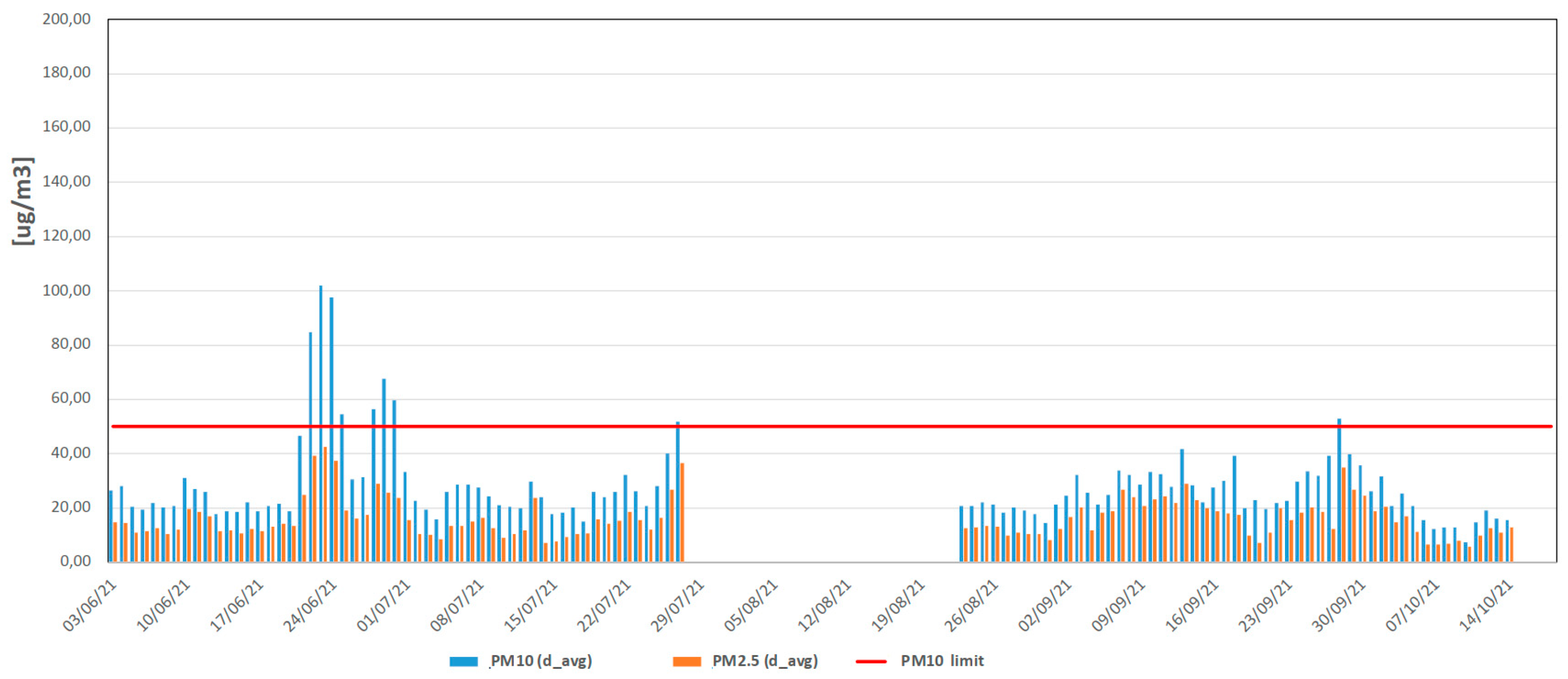
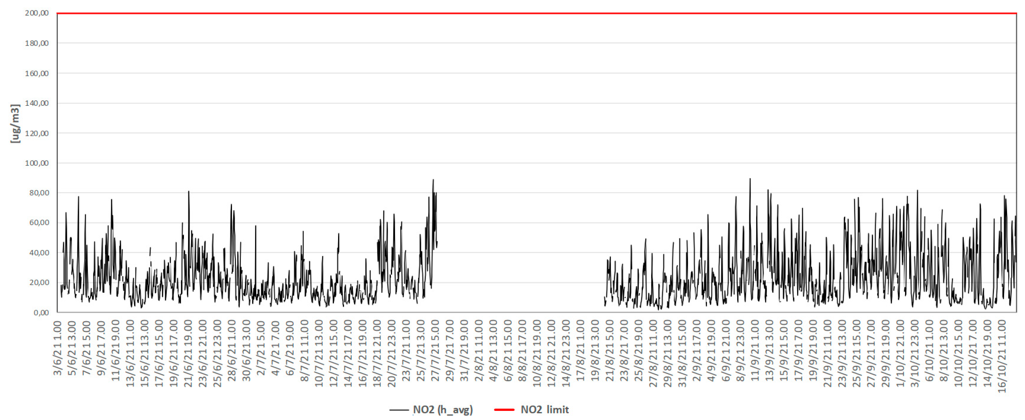
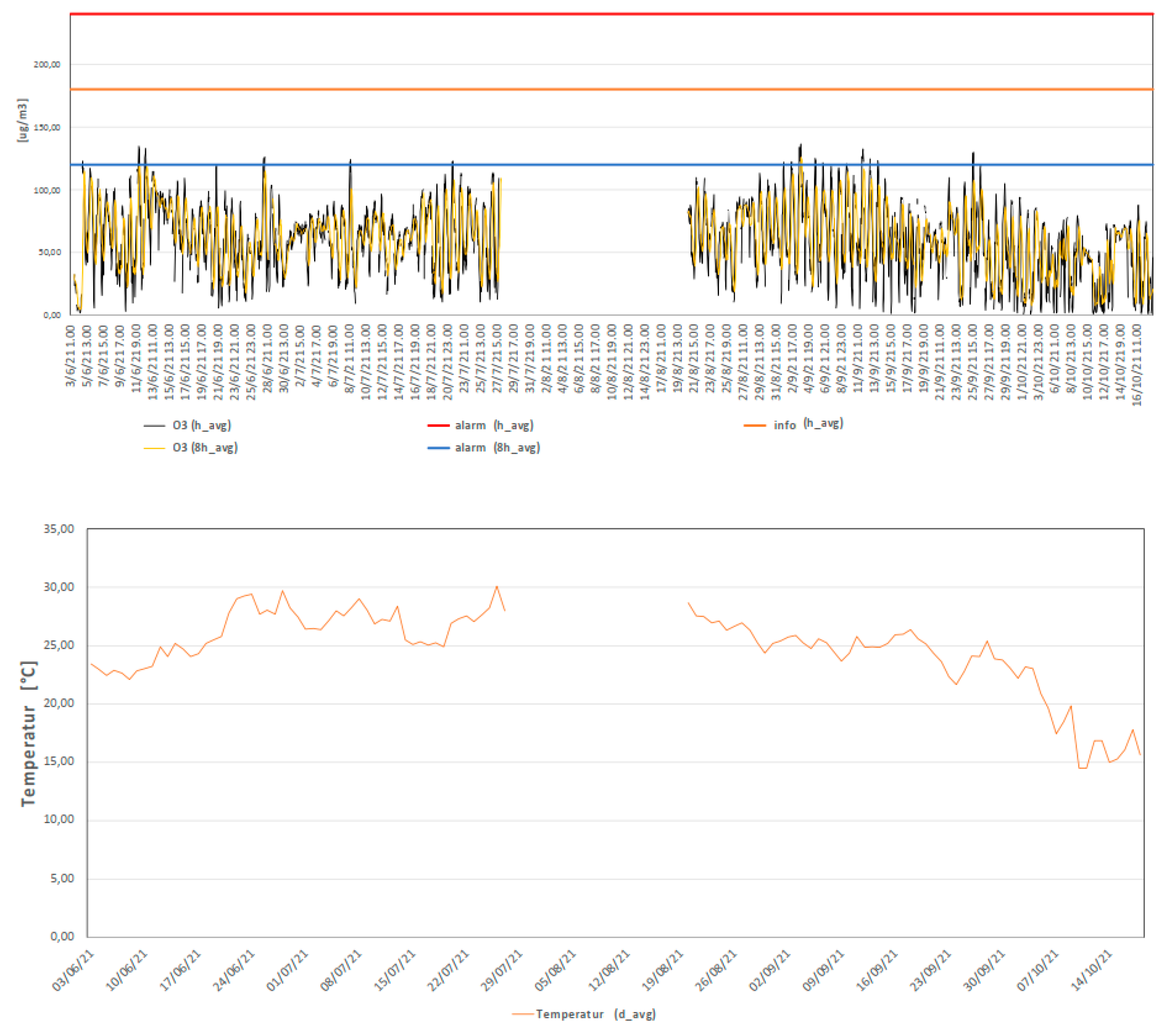
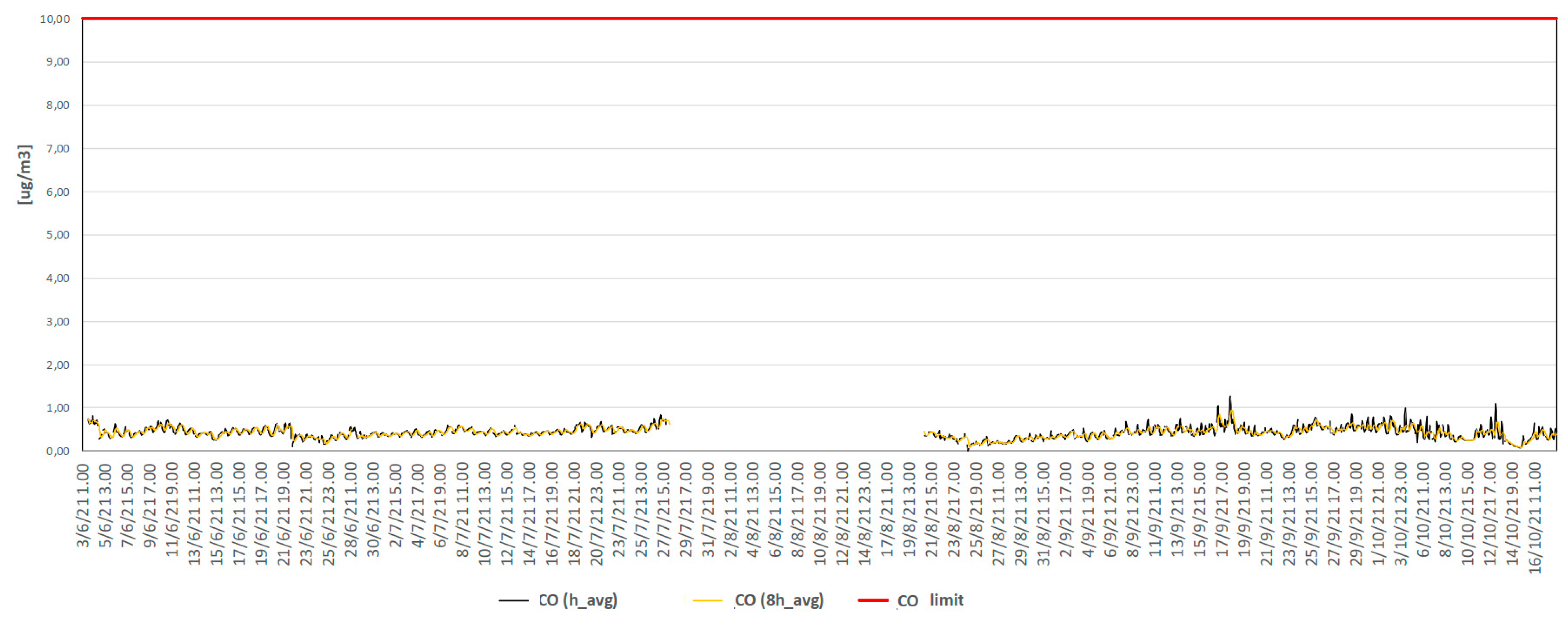
8.2. Second Co-Location Campaign: From 4 July 2021 to 4 October 2021 @ Portici Isola Ecologica

Particulate matter PM₁₀ and PM_2.5;

During the co-location period, the elevated levels of PM₁₀ observed in Figure 19 can be attributed to a substantial influx of Saharan dust, as indicated by the exceedances of the daily limit value. The discontinuity observed in the graph is a consequence of a period of interruption in the monitoring campaign.

Nitrogen Dioxide:

It can be confirmed that the concentration of the pollutant in question has never exceeded the legally prescribed limit value (red line in Figure 20) for the hourly average. Moreover, the typical upward trajectory is evident during the autumn months, when vehicular traffic intensifies due to the resumption of routine activities (such as work and schooling) commencing in September.

Ozone:

Figure 21 illustrates the pattern of hourly average O₃ concentrations (depicted in black) and 8 h moving averages (shown in yellow). From the graphs, a strong correlation between ozone concentration and temperature can be observed. For instance, the decline observed in October 2021 can be attributed to a reduction in the formation of ozone in the atmosphere, which is a consequence of the slowing down of the dissociation process of molecular oxygen and the formation of ozone.

Carbon Monoxide:

The CO concentrations during the specified period are within the expected range, as illustrated in Figure 22.

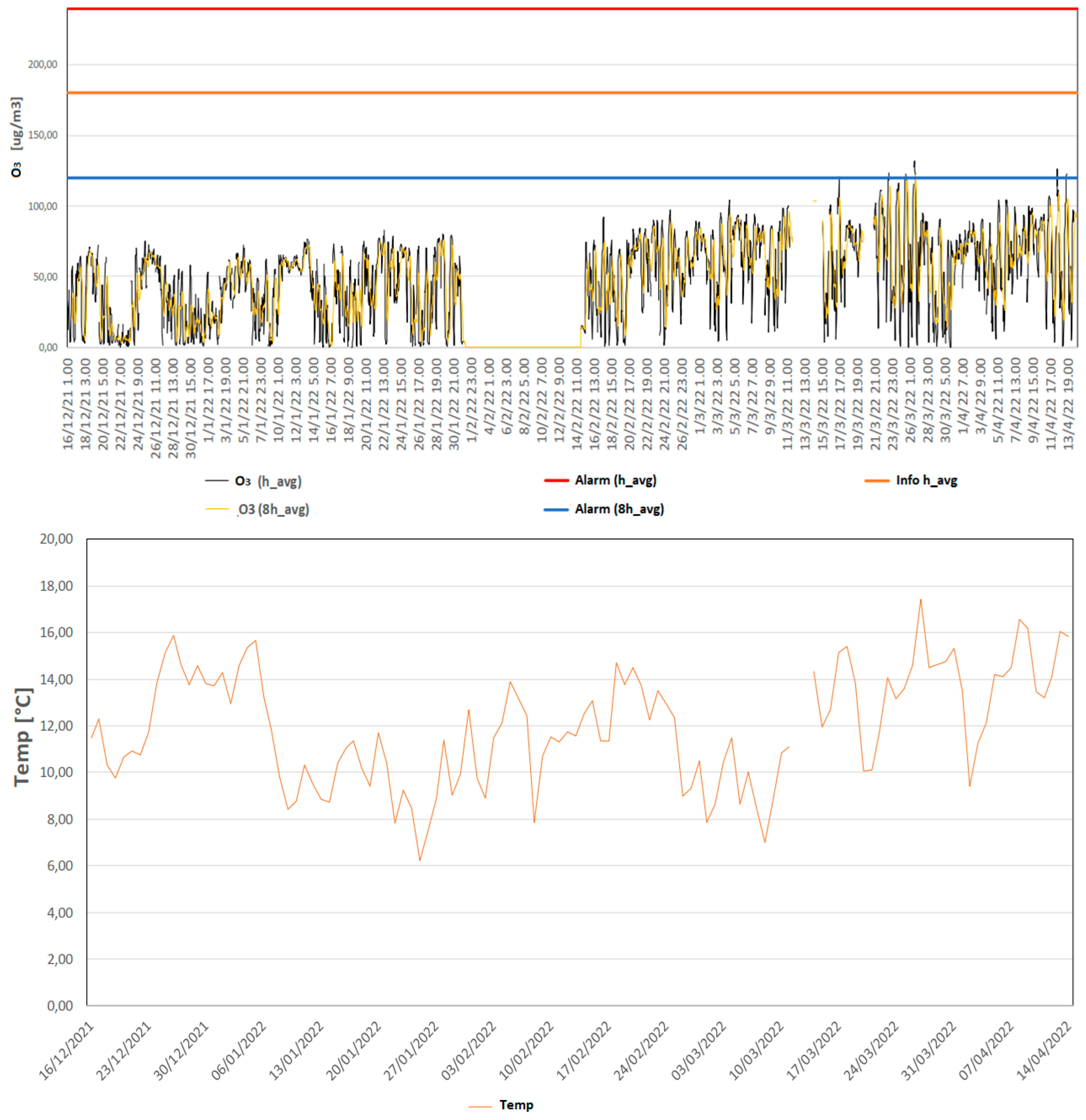
8.3. Third Co-Location Campaign: From 11 January 2022 to 12 April 2022 @ Portici Scuola Da Vinci Comes—Viale Bernini

Particulate matter PM₁₀ and PM_2.5:

Figure 23 shows the time series of daily average concentrations of PM₁₀ and PM_2.5 measured by the mobile laboratory station LM02 at the considered site. As can be easily seen, the number of exceedances of the daily PM₁₀ limit value recorded at site LM02 during the entire third co-location period is five, most of which occurred in December 2021, corresponding with New Year’s day.

Nitrogen Dioxide:

Even during the third co-location, no exceedance of the NO₂ limit has been recorded. Figure 24 shows the trend in hourly NO₂ concentrations measured by the LM02 mobile laboratory during the period under examination. Concentrations never exceeded the limit value for the hourly average concentration of 200 µg/m³ set by the regulations. On the other hand, the typical decreasing trend in concentrations in the spring months (when the emission contribution due to the operation of heating systems begins to disappear) is not particularly significant, which is an occurrence linked to the specific conditions of the site where emissions from vehicle traffic are predominant.

Ozone:

Figure 25 shows the trend in O₃ hourly average concentrations (black line) and the 8 h moving average (yellow line) for the LM02 mobile station. It can be seen that the ozone concentration is strongly dependent on temperature, e.g., there is a clear increasing trend in the change from winter to spring months.

Carbon Monoxide:

Also, for CO, the trend in concentrations is higher in the winter months, although well below the regulatory threshold values (Figure 26). This pattern aligns perfectly with what has been previously observed for other pollutants, such as nitrogen oxides.

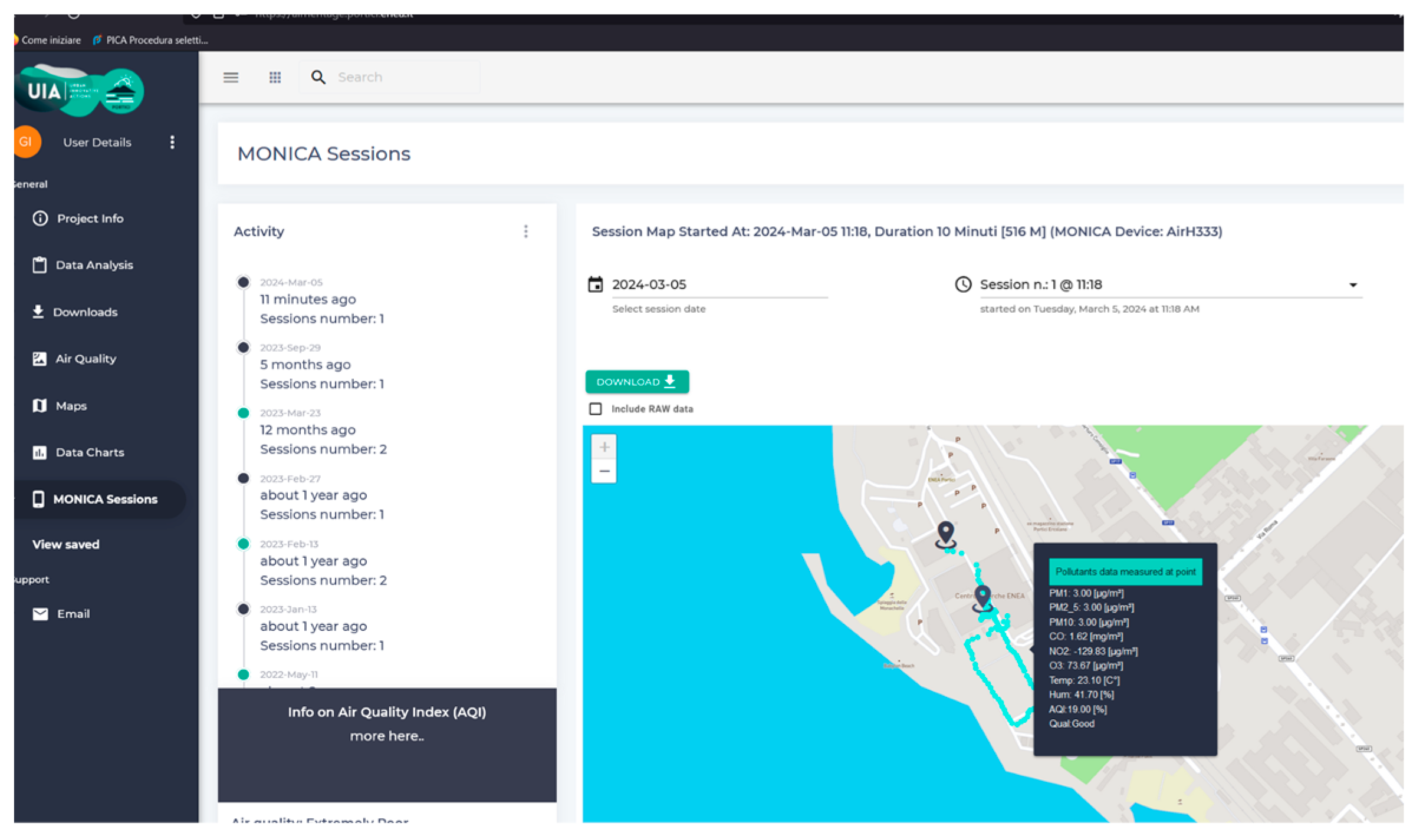
9. Citizen Engagement Through the MONICA App

9.1. Introduction and Role of the MONICA App in Citizen Engagement

Fixed stations enable us to measure the distributions of pollutants at a single geographical point. However, to observe how pollutants are spatially distributed over time, mobile campaigns can offer an interesting solution, optimizing the trade-off between spatial and temporal resolution. In this instance, volunteer citizens were enlisted for the implementation of mobile campaigns within the city of Portici. They literally “strolled” with MONICA through the city using armbands, backpacks, or little ad hoc bags, which left a completely open pathway to the MONICA inlet. The local associations, which were involved through the AirHeritage project partners, played a pivotal role in facilitating citizen involvement.

In order to guarantee the accurate transmission and storage of data collected by sensor nodes during citizen science campaigns, a dedicated smartphone application was developed. In essence, the user’s smartphone serves as a gateway between the sensor node and the web and, as we have seen, implements AI-based calibration algorithms reporting meaningful real-time exposure data.

The MONICA app is currently developed exclusively for Android smartphones using Android Studio. In order to ensure consistency with the developed IoT platform, Auth0 is employed for authentication services. Regarding distribution, we opted for third-party distribution, thereby making the .apk file accessible directly on a proper web page of the developed IoT platform (see Supplementary Materials).

Of course, not all end-users were previously familiar with the installation of third-party applications on their mobile device. Consequently, training events were organized to address this issue, which also included training in the use of the app and in the use of the web page for viewing the data of the sessions carried out. The user is able to access and view the data of their own sessions both from the back-end and on the appropriate screens of the app, as illustrated in Figure 27.

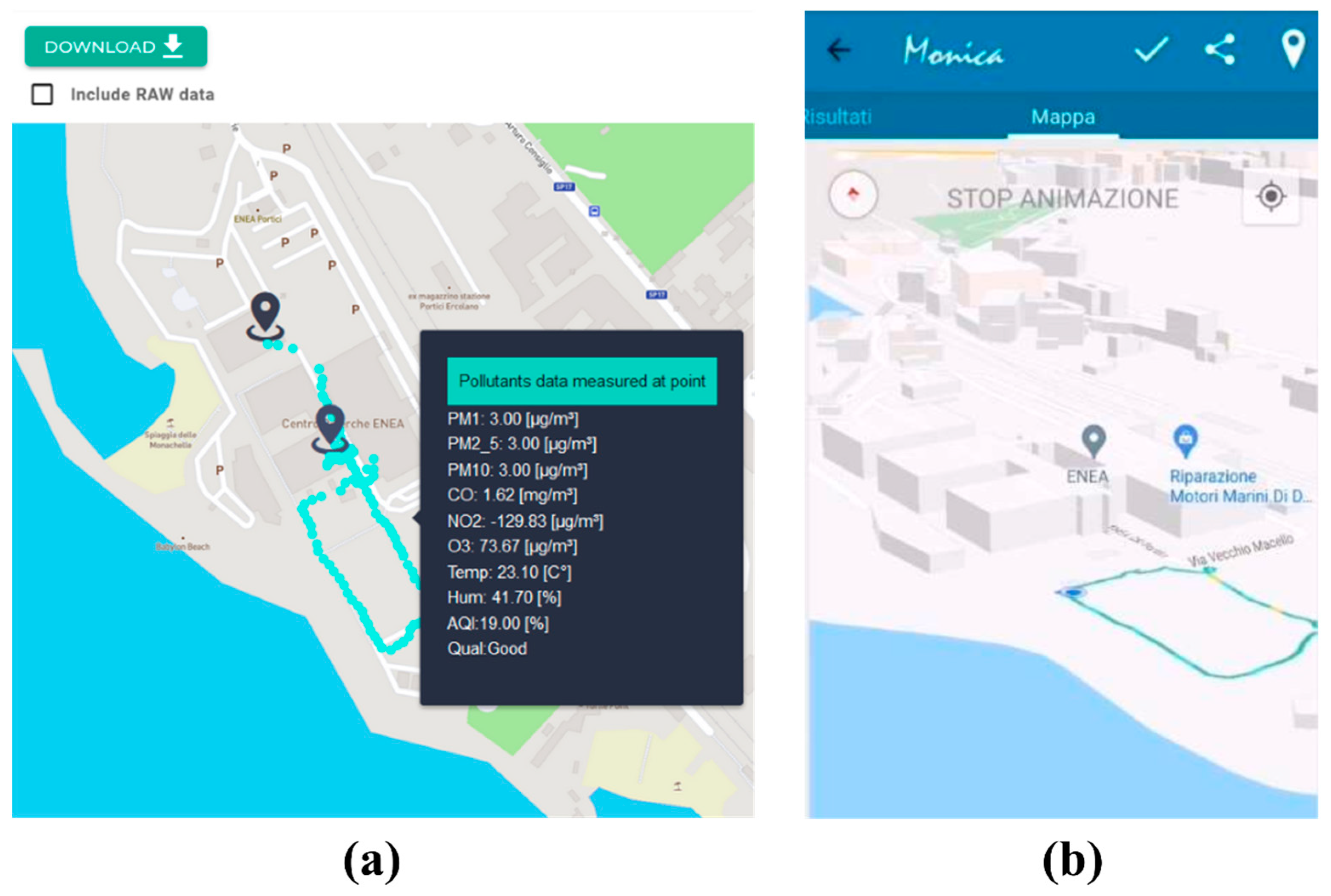
9.2. How the Monica App Works

The MONICA app is responsible for receiving sensor data via Bluetooth Low Energy (BLE), returning the concentration values relating to individual pollutants (calibrated data) and sending them together with the raw sensor data to the back-end server. Figure 28 provides a schematic representation of the data flow.

The unprocessed data from each MONICA sensor node are encapsulated in a JSON format and transmitted via BLE to the user’s smartphone. The BLEService class, as defined within the code, provides connection services with remote devices, intercepts and filters BLE communications, as well as routes these communications to the intended recipients. This enables the other components of the app to request actions from the BLEService. Unlike the location notification and update service, the BLEService is declared as an external background service. The calibration parameters, i.e., the MLR coefficients, are stored in a resource file called Linear Calibration, which is updated after each co-location with the new appropriate coefficients. Figure 29 delineates the sequence of operations comprising the comprehensive workflow, from the first co-location until the completion of the first citizen science campaign. The process is naturally repeated for each subsequent co-location.

An ad hoc developed function, BuildJSON, is responsible for the generation of a single JSON, which contains both the raw and calibrated data. Additionally, this function is responsible for creating the necessary sockets to send the raw data into the MongoDB raw data collection and the calibrated data into the MongoDB calibrated data collection.

The MONICA device was designed as a wearable device; therefore, it is not equipped with an internal memory card for storing the data of each individual session. Instead, the data must be sent to a remote server. In the event of a lack of network connectivity in specific locations during the monitoring session, there is a possibility of data loss. In order to prevent this situation, the app is capable of buffering the session data for two minutes. In the event that the network becomes available during this period, the buffered data are transmitted to the server in conjunction with the newly acquired data. In the event that the buffer is full and the network is not yet available, the session is closed proactively. In order to inform the user of the occurrence of such an event, we decided to display a “Toast message” on the smartphone screen. This message indicates whether the raw and calibrated data have been successfully transmitted to the server. Consequently, the user is able to take the necessary action to terminate the session and/or proceed to an alternative location where the network is accessible.

9.3. Feedback from the Citizen Science Campaigns

During the testing phase of the app and during the mobility campaigns, the app code was updated on a regular basis in order to ensure compatibility with the latest Android releases. This process was necessary in order to reach a stable version that would guarantee adequate compatibility. In order to familiarize users with the process of downloading and installing third-party apps on their smartphones, both virtual and in-person meetings have been provided. The management of the training phase of a large number of users and the concomitant updates to Android releases proved to be a significant challenge, requiring a significant expenditure of both time and human resources. The burden would have been significantly increased if we had decided to also develop an Apple version of the app and distribute it on their respective marketplaces. Nevertheless, this experience has led us to conclude that future app development should adopt multi-platform programming languages such as Flutter™ and distribute the app through the respective app stores.

It must be observed that the involvement of the general public in citizen science campaigns has been confined to a limited circle of volunteers from the participating associations and their acquaintances, largely engaged through word-of-mouth communication. The number of individuals from outside voluntary organizations who participated was negligible, despite extensive social media campaigns to advertise the campaigns. It would be beneficial to identify alternative methods of public engagement for future projects.

10. Impact of Spatial Analysis of Citizen-Generated Data

Capturing the local variability in air pollutant concentrations within the cities is a key issue to assess the urban air quality at a high spatial resolution as well as to evaluate the citizen exposure to high air pollution levels [10]. To address this issue within the project, a pervasive urban air quality monitoring technique using hybrid deployments of sensor networks has been investigated.

As shown in the literature, the high spatial variability of urban air pollution is not usually captured by regulatory monitoring networks, since they are sparsely distributed within the city. As a first task, the deployment of fixed low-cost sensor networks has been designed and developed across the pilot city of Portici.

Using networks of stationary low-cost sensors within a city, neighborhood-level differences as well as differences near specific sources (e.g., roadways) can be captured and pollutant spatial variations at fine (sub km) length scales can be quantified. At this scope, the relevant question of the “optimal sampling design” has been investigated. Thus, optimal sites for deploying stationary low-cost sensors have been identified and are aimed at spatially dense air pollution monitoring on the basis of which more reliable air quality forecasts across the city can be obtained; as well, population pollutant exposures can be evaluated more accurately.

To accomplish this, a spatial multicriteria analysis (GIS-Multi-Criteria Decision Assessment) has been developed for selecting suitable sites for low-cost multisensor traffic-orientated stations across the city. The process is detailed in [63].

Street canyon effects and traffic-related emissions were selected as suitability criteria, with the intention to represent the impact of local sources and land use on measured pollutant concentrations. In fact, street canyon effects, generated by the ratio between the building height and the street width, can modify concentration patterns near roadways. The traffic-related emissions contribute to background pollutant concentrations, but they are also the principal source of local variation in the concentrations of urban air pollutants. Higher pollutant concentrations are located in high traffic emission areas.

High- and low- traffic emission zones and hybrid zones were identified by a spatial hot spot analysis. All selected criteria were performed as geographical variables and combined in a weighted spatial overlay. For the pilot city of Portici, a map of suitable sites was generated for deploying low-cost multisensor traffic-orientated stations for monitoring and quantifying pollutant spatial variability in urban streets (Figure 30 and Figure 31).

Among the main results of this approach, we summarized the most relevant in the following list:

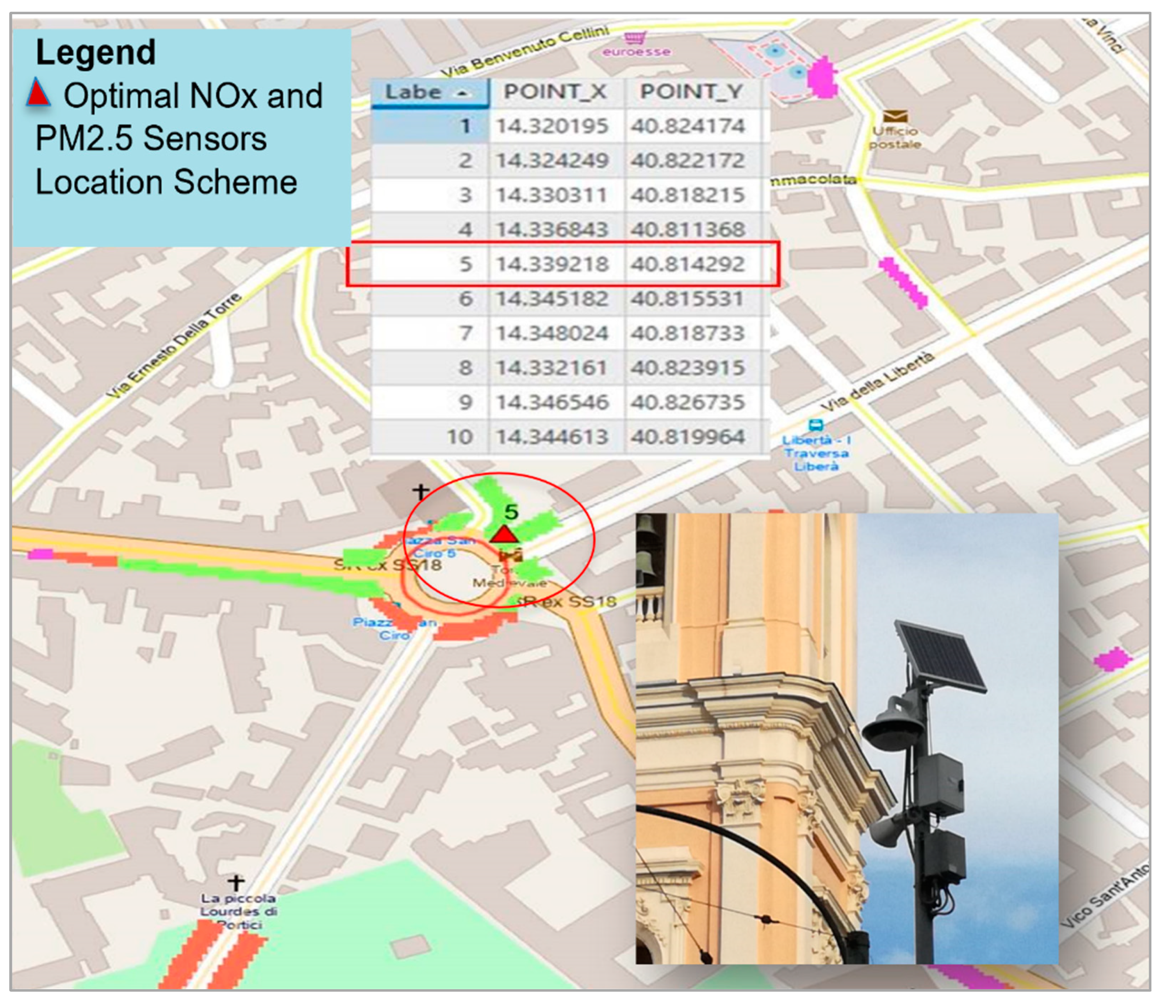
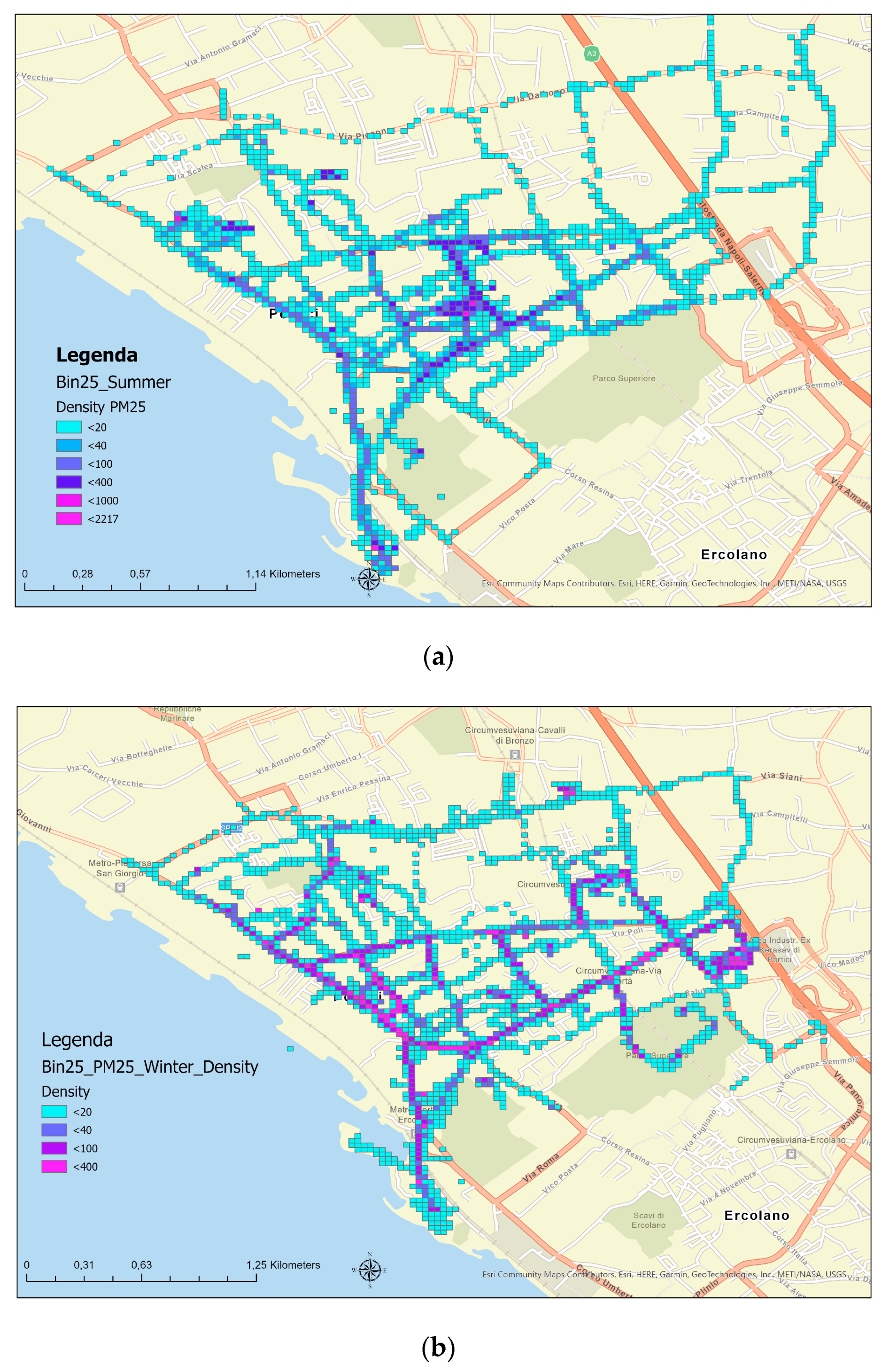
• Low-cost monitoring stations located at the eligible sites can convey information about areas on which space variability is significant, providing informative content which is actually lacking for both regulatory monitoring networks and modelling-based approaches for air quality mapping.
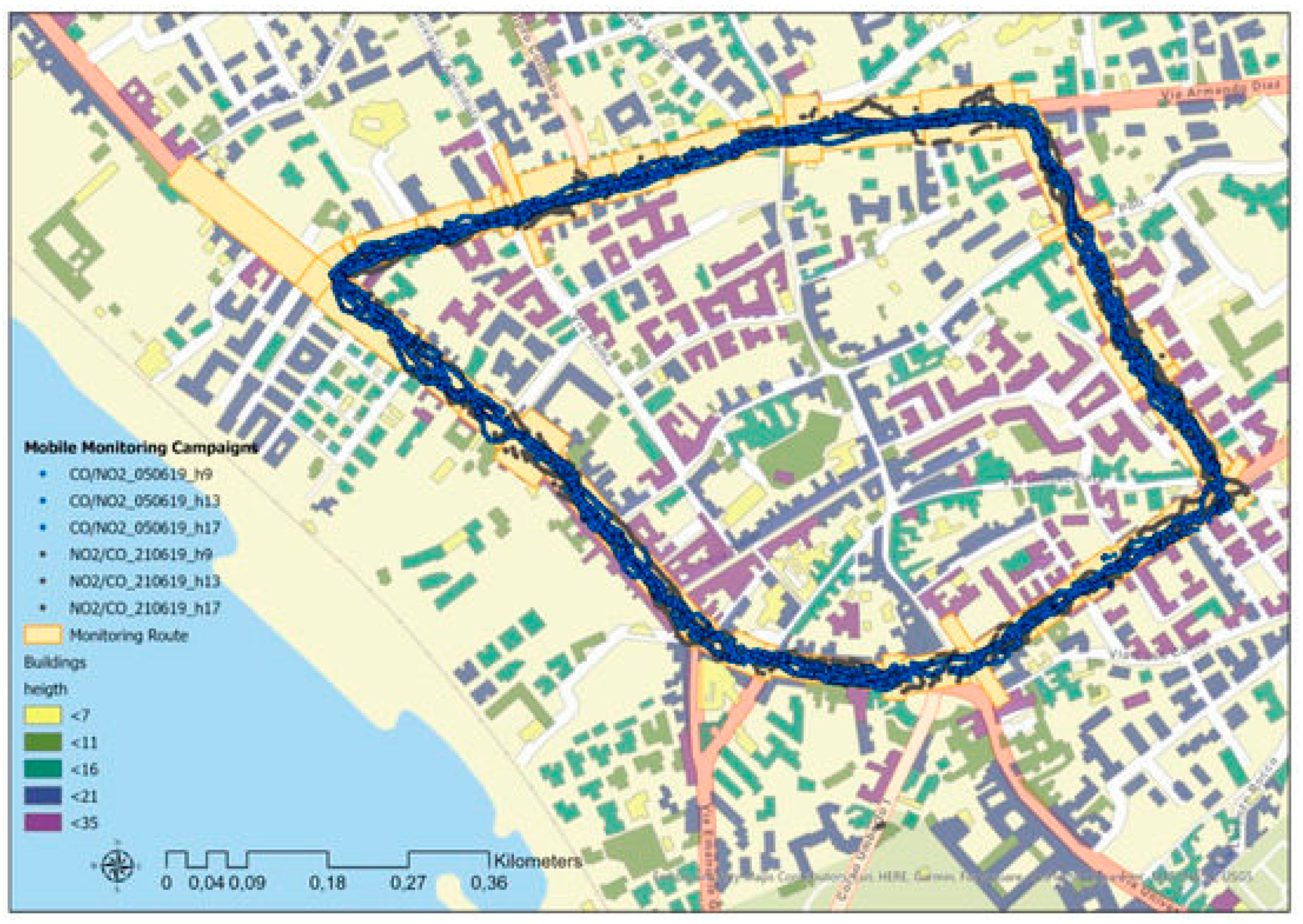
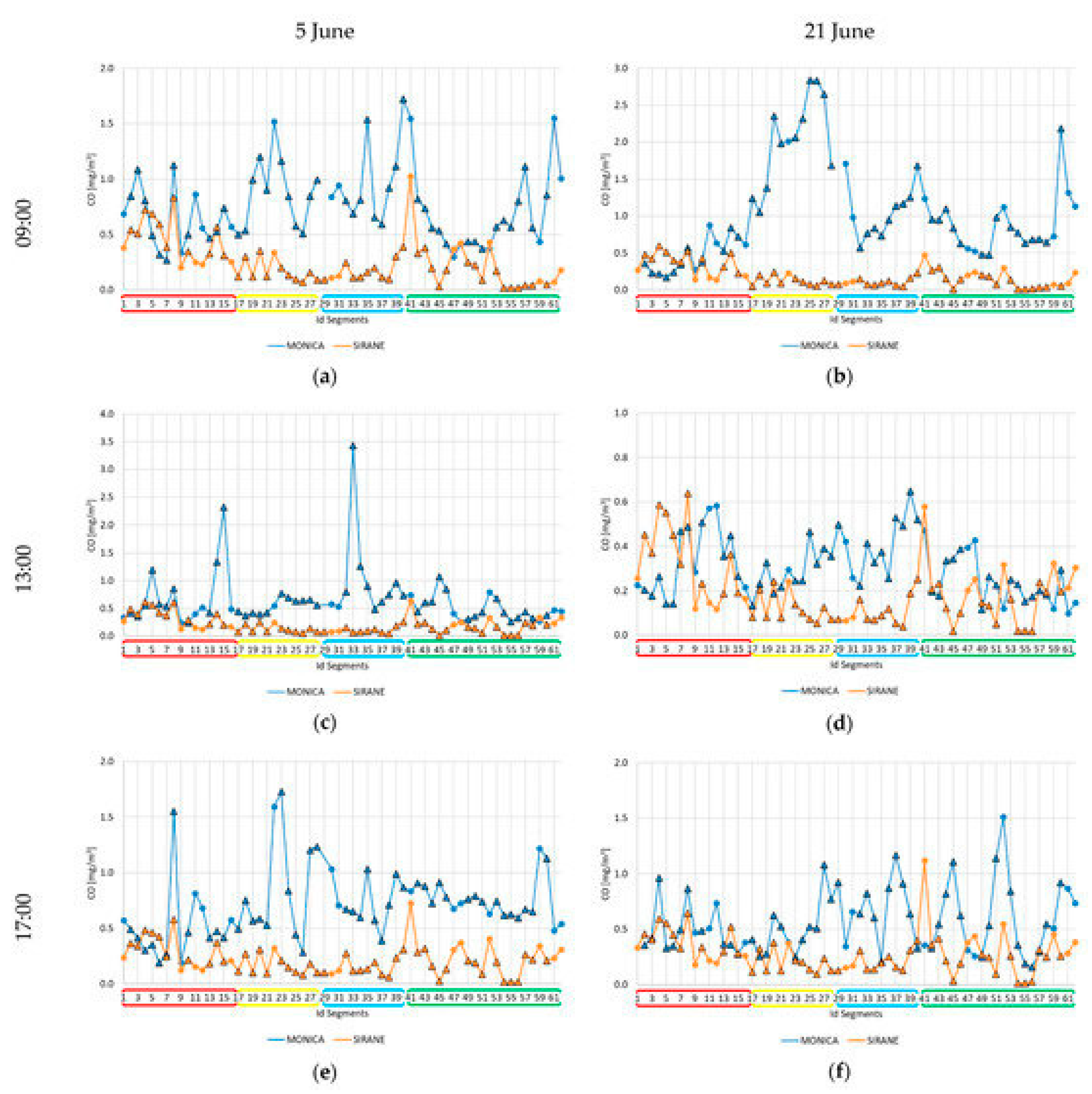
• In addition to the local spatial variability, the temporal variability of air pollutant concentrations has to be taken into account for obtaining more reliable urban air quality scenarios.
• One of the possible limitations to the use of the proposed spatial analysis is its reliance on data. Data could be difficult to obtain such as vehicular flow (simulated or measured) as well as the street canyon effects. In these cases, the use of proxy data could partially solve the issue.

Also, air quality data gathered by stationary low-cost (multi-) sensor networks as well as mobile and opportunistic monitoring campaigns across urban areas can be fundamental in data assimilation approaches aimed at including the variability patterns of air pollutant concentrations that conventional chemical transport models or land use regression models fail to adequately represent.

In this regard, we have investigated the capability of an operational air dispersion model at the district scale, such as SIRANE, in identifying the local spatio-temporal variability of pollutant concentrations within an urban district, with respect to mobile monitoring campaigns, using low-cost sensor devices—MONICA [64,65]. The campaign consisted of six runs, along a fixed monitoring route, repeated at two different days and different times on one day (Figure 32). By comparing the hourly average concentrations of CO and NO₂ pollutants collected by minute by MONICA devices and hourly concentrations simulated by SIRANE along the urban streets, we have shown that the recorded concentrations appear to exceed the simulated ones by a factor of three and two for CO and NO₂, respectively. Furthermore, for both the pollutants, this factor is higher within the street canyons than in open roads. However, the recorded data and the simulated pollutant concentrations show patterns that broadly correspond, and the peaks observed in the mobile profiles appear in the simulated profiles, though smoothed (Figure 33). The outcomes highlighted that there are differences between measured and estimated pollutant concentrations due to several factors. The operational conditions are one of these. MONICA measures pollutants concentrations at about 1 m height and at a high temporal resolution, also capturing concentration peaks due to events that occurred during the monitoring run such as a closely passing car or bus, or walking in the emission plume right behind a vehicle, or even idling vehicles due to local traffic congestion. SIRANE evaluates hourly concentrations, spatially averaged in each street segment.

A further task was to explore the potential of participatory monitoring campaigns for mapping the exposure to air pollution in the urban environment at a high spatial resolution. This monitoring approach made use of citizens’ common daily routines to move low-cost air quality measurement devices as MONICA around the city. It is a promising approach based on an unstructured setup to collect large datasets that give useful additional information at a reasonable cost compared to classical data collection methods. But, depending on the setup of the data collection, such new data can lead to new challenges in data processing and interpretation. In this regard, a statistical analysis method, spatial binning, was applied in an original way for exploring the distribution of the large dataset collected by the citizens carrying MONICA devices during their daily walking routes around the city; this results in unstructured measurements without distinct patterns in space or time.

The collected measurements were grouped in a summer (from April to July) campaign and a winter (from October to December) campaign on most of the urban roads. About 46,000 raw 5 s measurements of CO, NO₂, O₃, PM_2.5, and PM₁₀ concentrations were recorded during the summer campaign and about 100,000 raw 5 s measurements of the same pollutants were recorded during the winter campaign. Most of the measurements were recorded between 8 a.m. and 5 p.m. during working days. The study area covers approximately 4 km².

For the distribution analysis of these opportunistic measurements, the data were spatially aggregated within bins of 25 × 25 m, located along the street networks, and median statistics were calculated. To assure data quality, the calculated median was based on at least 20 measurements. Maps of the measurement density for each bin and for each recoded pollutant were performed (Figure 34). Similarly, maps of the distribution (median value) of the recorded pollutant concentrations within the 25 m bins were performed (Figure 35) and categorized as good, fair, moderate, or poor. Most of pollutant concentration measurements fall in the moderate and poor classes in winter campaign, while in the summer campaign they mainly fall in good and fair classes.

Potential Improvements for Future Geostatistical Studies

Factors that can impact on the site eligibility for low-cost multisensor monitors could be considered as further location constraints, such as the shadow effect of buildings and trees as well as the evaluation of the minimum winter solar radiation value. In fact, low-cost monitors are generally equipped with a photovoltaic panel and a battery storage area and installed on existing street lighting poles. Including these constraints should allow us to select sites with better sun exposure over the year. Furthermore, the use of MONICA devices at different heights as well as opportunistic and more pervasive monitoring campaigns could improve the understanding of the differences between measured and modelled concentrations. Thus, a limited number of measurements and sampling errors impact the uncertainty of concentration level distributions, although large spatial patterns within the city are also captured. The deployment of unstructured opportunistic mobile monitoring, coupled with repeated measurements and a meticulous approach to data processing and interpretation, is of paramount importance. This monitoring strategy must be capable of collecting a substantial amount of data, encompassing both spatial and temporal variability across the city. Until low-cost air quality sensors are developed that can collect data of sufficient quality in an effortless manner, it is imperative to maintain motivation and follow-up with participants.

11. Conclusions

The AirHeritage project was devised to tackle the needs of a medium-sized city with a high-density population, where air quality is significantly affected by anthropic effects and with no continuous regulatory grade information about pollutant concentrations. The proposed technical solution was to devise, deploy, and test a hierarchical, hybrid (fixed and mobile) network of low-cost air quality multisensory devices, mixing participatory mobile and stationary monitoring approaches so as to obtain ultra-high-resolution spatial pollutant maps. This research allowed us to openly review the design choices and the outcomes deriving guidance, which we perceive to be of interest to the distributed air quality sensing community at large. Feasibility, sustainability, and accuracy challenges, and the respective proposed solutions have been discussed in different focused sections. All the choices have been driven by the accurate description of the project goals and operative scenario; this allowed us to select the appropriate network design and define the functional and operative requirements. This phase undoubtedly emerged as the most important and challenging. While accuracy is one of the significant requirements in many scenarios, the inherent limitations of the available sensing technology must be taken into account in AQ data communication, to avoid unrealistic expectations. Actually, the presented devices are undoubtfully less accurate than the regulatory grade and so-called equivalent measurement methods. Limitations may be effectively tackled and remediated in the short term with adequate data-driven calibration strategies, considering data gathering, access to reference station data, relocation issues, and lastly, AI models. Despite the ad hoc optimization of the calibration parameters, the performance variance expressed by the nodes is relevant and must be taken into account during data fusion. The logistics of such ad hoc repeated calibration solution costs may easily become prohibitive without resorting to advanced techniques. These include universal and remote calibration strategies. Both are still to be extensively tested while already commercially available. Moving resources towards continuous calibration strategies, the so-called golden node calibration strategy may become useful, especially when the number of measuring points is limited. Among the software functional requirements, the possibility to obtain an immediate personal exposure response has been considered the most important by users. IoT ecosystems are continuously being updated, with new functionalities becoming available and easily deployable; among these, the possibility for implementing edge computing facilities should be considered paramount for LCAQMSs. The use of geomatic tools has allowed us to determine an optimal deployment strategy and to grasp the expected modeled spatial variance with a limited number of fixed stations. We would like to stress the need for the adequate preprocessing of mobile-gathered data, both for tackling the influence of the sensor response time on location imputed data, and for building realistic and informative pollutant concentration maps. Opportunistic measurements are desirable from the user’s point of view but may easily determine a largely non-uniform distribution in terms of location and hour of the days. The transferability of these findings is guaranteed in similar scenarios, which are rather common in southern EU. In scenarios where industrial pollution becomes significant, a different choice of the monitored parameters will be extremely important to obtain the relevant information and to enable source apportionment. Where no fixed deployment is foreseen, establishing a mixed strategy combining opportunistic and prescheduled paths and timing can help reduce the data skewing; such a strategy is suggested in [66].

We think that the reported insights can be of value for the community and may help cities and companies to properly design future monitoring network as well as carefully consider the data-gathering strategy. To this end, we hope that the sharing of the AirHeritage datalake may further help to experiment with different approaches and continue to extract value from the gathered data.

References

1. WHO. World Health Statistics 2022, Monitoring Health for the SDGs, Sustainable Development Goals; World Health Organization: Geneva, Switzerland, 2022. [Google Scholar]
2. Pascal, M.; Corso, M.; Chanel, O.; Declercq, C.; Badaloni, C.; Cesaroni, G.; Henschel, S.; Meister, K.; Haluza, D.; Martin-Olmedo, P.; et al. Assessing the public health impacts of urban air pollution in 25 European cities: Results of the Aphekom project. Sci. Total Environ. 2013, 449, 390–400. [Google Scholar] [CrossRef] [PubMed]
3. Medina, S.; Adélaïde, L.; Wagner, V.; de Crouy Chanel, P.; Real, E.; Colette, A.; Couvidat, F.; Bessagnet, B.; Duron, A.; Host, S.; et al. Impact de Pollution de L’air Ambiant sur la Mortalité en France Métropolitaine RÉDUCTION en Lien Avec le Confinement du Printemps 2020 et Nouvelles Données sur le Poids Total Pour la Période 2016–2019; Santé publique: Paris, France, 2021; p. 63. [Google Scholar]
4. Wu, S.; Ni, Y.; Li, H.; Pan, L.; Yang, D.; Baccarelli, A.A.; Deng, F.; Chen, Y.; Shima, M.; Guo, X. Short-term exposure to high ambient air pollution increases airway inflammation and respiratory symptoms in chronic obstructive pulmonary disease patients in Beijing, China. Environ. Int. 2016, 94, 76–82. [Google Scholar] [CrossRef] [PubMed]
5. Raaschou-Nielsen, O.; Beelen, R.; Wang, M.; Hoek, G.; Andersen, Z.; Hoffmann, B.; Stafoggia, M.; Samoli, E.; Weinmayr, G.; Dimakopoulou, K.; et al. Particulate matter air pollution components and risk for lung cancer. Environ. Int. 2015, 87, 66–73. [Google Scholar] [CrossRef] [PubMed]
6. Latza, U.; Gerdes, S.; Baur, X. Effects of nitrogen dioxide on human health: Systematic review of experimental and epidemiological studies conducted between 2002 and 2006. Int. J. Hyg. Environ. Health 2009, 212, 271–287. [Google Scholar] [CrossRef]
7. Kim, S.-Y.; Kim, E.; Kim, W.J. Health Effects of Ozone on Respiratory Diseases. Tuberc. Respir. Dis. 2020, 83 (Suppl. S1), S6–S11. [Google Scholar] [CrossRef] [PubMed] [PubMed Central]
8. Zhang, L.-W.; Chen, X.; Xue, X.-D.; Sun, M.; Han, B.; Li, C.-P.; Ma, J.; Yu, H.; Sun, Z.-R.; Zhao, L.-J.; et al. Long-term exposure to high particulate matter pollution and cardiovascular mortality: A 12-year cohort study in four cities in northern China. Environ. Int. 2013, 62, 41–47. [Google Scholar] [CrossRef]
9. Díaz-Robles, L.A.; Fu, J.S.; Reed, G.D. Emission scenarios and the health risks posed by priority mobile air toxics in an urban to regional area: An application in Nashville, Tennessee. Aerosol. Air. Qual. Res. 2013, 13, 795–803. [Google Scholar] [CrossRef]
10. Testi, I.; Wang, A.; Paul, S.; Mora, S.; Walker, E.; Nyhan, M.; Duarte, F.; Santi, P.; Ratti, C. Big mobility data reveals hyperlocal air pollution exposure disparities in the Bronx, New York. Nat. Cities 2024, 1, 512–521. [Google Scholar] [CrossRef]
11. Castell, N.; Kobernus, M.; Liu, H.Y.; Schneider, P.; Lahoz, W.; Berre, A.J.; Noll, J. Noll Mobile technologies and services for environ-mental monitoring: The Citi-Sense-MOB approach. Urban Clim. 2015, 14, 370–382. [Google Scholar] [CrossRef]
12. Enhance Environmental Awareness Through Social Information Technologies. Available online: https://cordis.europa.eu/project/id/265432/it (accessed on 1 October 2024).
13. Available online: https://cordis.europa.eu/article/id/175088-citizenbased-air-quality-monitoring (accessed on 1 October 2024).
14. Stojanović, D.B.; Kleut, D.; Davidović, M.; Živković, M.; Ramadani, U.; Jovanović, M.; Lazović, I.; Jovašević-Stojanović, M. Data Evaluation of a Low-Cost Sensor Network for Atmospheric Particulate Matter Monitoring in 15 Municipalities in Serbia. Sensors 2024, 24, 4052. [Google Scholar] [CrossRef]
15. Breathe London. Available online: https://www.breathelondon.org/about (accessed on 1 October 2024).
16. Castell, N.; Dauge, F.R.; Schneider, P.; Vogt, M.; Lerner, U.; Fishbain, B.; Broday, D.; Bartonova, A. Can commercial low-cost sensor platforms contribute to air quality monitoring and exposure estimates? Environ. Int. 2017, 99, 293–302. [Google Scholar] [CrossRef] [PubMed]
17. Bossche, J.V.D.; Theunis, J.; Elen, B.; Peters, J.; Botteldooren, D.; De Baets, B. Opportunistic mobile air pollution monitoring: A case study with city wardens in Antwerp. Atmos. Environ. 2016, 141, 408–421. [Google Scholar] [CrossRef]
18. AirVisual. Available online: https://www.indiegogo.com/projects/airvisual-node-the-world-s-smartest-air-monitor#/ (accessed on 1 October 2024).
19. Chukwu, T.M.; Morse, S.; Murphy, R.J. Air quality perceptual index approach: Development and application with data from two Nigerian cities. Environ. Sustain. Indic. 2024, 23, 100418. [Google Scholar] [CrossRef]
20. UIA AirHeritage Project Description Page. Available online: https://www.uia-initiative.eu/en/operational-challenges/portici-air-heritage (accessed on 1 August 2024).
21. Alphasense UK Website. Available online: https://www.alphasense.com (accessed on 1 August 2024).
22. Plantower Company Website. Available online: https://www.plantower.com (accessed on 1 August 2024).
23. Teledyne API Website. Available online: https://www.teledyne-api.com/products/nitrogen-compound-instruments/t200 (accessed on 1 August 2024).
24. DIGITECO srl Website. Available online: https://www.digiteco.it (accessed on 1 August 2024).
25. Feng, Z.; Zheng, L.; Ren, B.; Liu, D.; Huang, J.; Xue, N. Feasibility of Low-Cost Particulate Matter Sensors For Long-Term Environmental Monitoring: Field Evaluation and Calibration. Sci. Total. Environ. 2024, 945, 174089. [Google Scholar] [CrossRef] [PubMed]
26. Wang, Y.; Du, Y.; Wang, J.; Li, T. Calibration of a Low-Cost Pm2.5 Monitor Using a Random Forest Model. Environ. Int. 2019, 133, 105161. [Google Scholar] [CrossRef]
27. Cordero, J.M.; Borge, R.; Narros, A. Using Statistical Methods to Carry out in Field Calibrations of Low Cost Air Quality Sensors. Sens. Actuators B Chem. 2018, 267, 245–254. [Google Scholar] [CrossRef]
28. Sá, J.; Chojer, H.; Branco, P.; Alvim-Ferraz, M.; Martins, F.; Sousa, S. Two Step Calibration Method For Ozone Low-Cost Sensor: Field Experiences with the UrbanSense DCUs. J. Environ. Manag. 2023, 328, 116910. [Google Scholar] [CrossRef]
29. Wilkinson, M.D.; Dumontier, M.; Aalbersberg, I.J.; Appleton, G.; Axton, M.; Baak, A.; Blomberg, N.; Boiten, J.W.; da Silva Santos, L.B.; Bourne, P.E.; et al. The Fair Guiding Principles for Scientific Data Management and Stewardship. Sci. Data 2016, 3, 160018. [Google Scholar] [CrossRef]
30. What Is REST? REST API Tutorial. Available online: https://restfulapi.net/ (accessed on 29 June 2024).
31. Lei, Z.; Zhou, H.; Ye, S.; Hu, W.; Liu, G.-P. Cost-Effective Server-side Re-deployment for Web-based Online Laboratories Using NGINX Reverse Proxy. IFAC-PapersOnline 2020, 53, 17204–17209. [Google Scholar] [CrossRef]
32. Bourhis, P.; Reutter, J.L.; Vrgoč, D. JSON: Data model and query languages. Inf. Syst. 2019, 89, 101478. [Google Scholar] [CrossRef]
33. How to Get Started with Node.js and Express|DigitalOcean. Available online: https://www.digitalocean.com/community/tutorials/nodejs-express-basics (accessed on 29 June 2024).
34. Singh, J.; Chaudhary, N.K. OAuth 2.0: Architectural Design Augmentation for Mitigation of Common Security Vulnerabilities. J. Inf. Secur. Appl. 2022, 65, 103091. [Google Scholar] [CrossRef]
35. Auth0 Overview. Available online: https://auth0.com/docs/get-started/auth0-overview (accessed on 29 June 2024).
36. Register Machine-to-Machine Applications. Available online: https://auth0.com/docs/get-started/auth0-overview/create-applications/machine-to-machine-apps (accessed on 29 June 2024).
37. Change Streams & Triggers with Node.js Tutorial|MongoDB. Available online: https://www.mongodb.com/developer/languages/javascript/nodejs-change-streams-triggers/ (accessed on 29 June 2024).
38. Shahzad, F. Modern and Responsive Mobile-enabled Web Applications. Procedia Comput. Sci. 2017, 110, 410–415. [Google Scholar] [CrossRef]
39. Liu, H.; Li, Q.; Yu, D.; Gu, Y. Air Quality Index and Air Pollutant Concentration Prediction Based on Machine Learning Algorithms. Appl. Sci. 2019, 9, 4069. [Google Scholar] [CrossRef]
40. De Vito, S.; Esposito, E.; D’Elia, G.; Del Giudice, A.; Fattoruso, G.; Ferlito, S.; D’Auria, P.; Intini, F.; Di Francia, G.; Terzini, E. High Resolution Air Quality Monitoring with IoT Intelligent Multisensor Devices During COVID-19 Pandemic Phase 2 in Italy. In Proceedings of the 12th AEIT International Annual Conference (AEIT), Catania, Italy, 23–25 September 2020. [Google Scholar]
41. Building with Patterns: The Bucket Pattern|MongoDB. Available online: https://www.mongodb.com/developer/products/mongodb/bucket-pattern/ (accessed on 29 June 2024).
42. Efficient Error Monitoring: Integrating Sentry in Node.js, Express.js, and MongoDB Backend Rest API Project|Widle Studio LLP. Available online: https://medium.com/widle-studio/enhancing-error-tracking-and-monitoring-integrating-sentry-in-node-js-3f827deffca5 (accessed on 29 June 2024).
43. How to Protect an Nginx Server with Fail2Ban on Ubuntu 20.04|Digital Ocean. Available online: https://www.digitalocean.com/community/tutorials/how-to-protect-an-nginx-server-with-fail2ban-on-ubuntu-20-04 (accessed on 29 June 2024).
44. Is Protobuf Much Faster than Json Even in Simple Web Server Response Requests?|by Kuentra Official|Medium. Available online: https://medium.com/@kn2414e/is-protocol-buffers-protobuf-really-lighter-and-faster-compared-to-json-681c6bee5d93 (accessed on 29 June 2024).
45. Masdani, M.V.; Darlis, D. A Comprehensive Study on Mqtt as a Low Power Protocol for Internet of Things Application. IOP Conf. Series Mater. Sci. Eng. 2018, 434, 012274. [Google Scholar] [CrossRef]
46. Time Series Collection Limitations—MongoDB Manual v7.0. Available online: https://www.mongodb.com/docs/manual/core/timeseries/timeseries-limitations/ (accessed on 29 June 2024).
47. Improving Scalability of Cloud-Based IoT Application with Microservice Architecture Using Massively Distributed Kuber-Netes Cluster|Request PDF. Available online: https://www.researchgate.net/publication/346443549_Improving_Scalability_of_Cloud-based_IoT_Application_with_Microservice_Architecture_using_Massively_Distributed_Kubernetes_Cluster (accessed on 29 June 2024).
48. Rani, F.; Wang, X.; Mutlu, I.; Urbas, L. A Centralized MongoDB-Based Repository Design for IIoT Data: The ecoKI Project*. IFAC-PapersOnLine 2023, 56, 3184–3189. [Google Scholar] [CrossRef]
49. Schneider, P.; Vogt, M.; Haugen, R.; Hassani, A.; Castell, N.; Dauge, F.R.; Bartonova, A. Deployment and Evaluation of a Network of Open Low-Cost Air Quality Sensor Systems. Atmosphere 2023, 14, 540. [Google Scholar] [CrossRef]
50. Malings, C.; Tanzer, R.; Hauryliuk, A.; Kumar, S.P.N.; Zimmerman, N.; Kara, L.B.; Presto, A.A.; Subramanian, R. Development of a general calibration model and long-term performance evaluation of low-cost sensors for air pollutant gas monitoring. Atmos. Meas. Tech. 2019, 12, 903–920. [Google Scholar] [CrossRef]
51. De Vito, S.; D’Elia, G.; Di Francia, G. Global calibration models match ad-hoc calibrations field performances in low cost particulate matter sensors. In Proceedings of the 2022 IEEE International Symposium on Olfaction and Electronic Nose (ISOEN), Aveiro, Portugal, 29 May–1 June 2022; pp. 1–4. [Google Scholar]
52. Smith, K.R.; Edwards, P.M.; Ivatt, P.D.; Lee, J.D.; Squires, F.; Dai, C.; Peltier, R.E.; Evans, M.J.; Sun, Y.; Lewis, A.C. An Im-proved Low-Power Measurement of Ambient NO2 and O3 Combining Electrochemical Sensor Clusters and Machine Learning. Atmos. Meas. Tech. 2019, 12, 1325–1336. [Google Scholar] [CrossRef]
53. Swager, T.M.; Mirica, K.A. Introduction: Chemical Sensors. Chem. Rev. 2019, 119, 1–2. [Google Scholar] [CrossRef]
54. D’Elia, G.; Ferro, M.; Sommella, P.; De Vito, S.; Ferlito, S.; D’Auria, P.; Di Francia, G. Influence of Concept Drift on Metrological Performance of Low-Cost NO2 Sensors. IEEE Trans. Instrum. Meas. 2022, 71, 1–11. [Google Scholar] [CrossRef]
55. Casey, J.G.; Hannigan, M.P. Testing the performance of field calibration techniques for low-cost gas sensors in new de-ployment locations: Across a county line and across Colorado. Atmos. Meas. Tech. 2018, 11, 6351–6378. [Google Scholar] [CrossRef]
56. Vikram, S.; Collier-Oxandale, A.; Ostertag, M.H.; Menarini, M.; Chermak, C.; Dasgupta, S.; Rosing, T.; Hannigan, M.; Griswold, W.G. Evaluating and improving the reliability of gas-phase sensor system calibrations across new locations for ambient measurements and personal exposure monitoring. Atmos. Meas. Tech. 2019, 12, 4211–4239. [Google Scholar] [CrossRef]
57. De Vito, S.; Esposito, E.; Massera, E.; Formisano, F.; Fattoruso, G.; Ferlito, S.; Del Giudice, A.; D’elia, G.; Salvato, M.; Polichetti, T.; et al. Crowdsensing IoT Architecture for Pervasive Air Quality and Exposome Monitoring: Design, Development, Calibration, and Long-Term Validation. Sensors 2021, 21, 5219. [Google Scholar] [CrossRef] [PubMed]
58. De Vito, S.; D’elia, G.; Ferlito, S.; Di Francia, G.; Davidović, M.D.; Kleut, D.; Stojanović, D.; Jovaševic-Stojanović, M. A Global Multiunit Calibration as a Method for Large-Scale IoT Particulate Matter Monitoring Systems Deployments. IEEE Trans. Instrum. Meas. 2023, 73, 1–16. [Google Scholar] [CrossRef]
59. Zimmerman, N.; Presto, A.A.; Kumar, S.P.N.; Gu, J.; Hauryliuk, A.; Robinson, E.S.; Robinson, A.L.; Subramanian, R. A ma-chine learning calibration model using random forests to improve sensor performance for lower-cost air quality monitoring. Atmos. Meas. Tech. 2018, 11, 291–313. [Google Scholar] [CrossRef]
60. Ramel-Delobel, M.; Peruzzi, C.; Coudon, T.; De Vito, S.; Fattoruso, G.; Praud, D.; Fervers, B.; Salizzoni, P. Exposure to airborne particulate matter during commuting using portable sensors: Effects of transport modes in a French metropolis study case. J. Environ. Manag. 2024, 365, 121400. [Google Scholar] [CrossRef]
61. Miskell, G.; Alberti, K.; Feenstra, B.; Henshaw, G.S.; Papapostolou, V.; Patel, H.; Polidori, A.; Salmond, J.A.; Weissert, L.; Williams, D.E. Reliable data from low cost ozone sensors in a hierarchical network. Atmos. Environ. 2019, 214, 116870. [Google Scholar] [CrossRef]
62. De Vito, S.; Elia, G.D.; Ferlito, S.; Esposito, E.; Piantadosi, G.; Di Francia, G. Remote Calibration strategies for Low Cost Air Quality Multisensors: A performance comparison. In Proceedings of the 2024 IEEE International Symposium on Olfaction and Electronic Nose (ISOEN), Grapevine, TX, USA, 12–15 May 2024; pp. 1–4. [Google Scholar]
63. Fattoruso, G.; Nocerino, M.; Toscano, D.; Pariota, L.; Sorrentino, G.; Manna, V.; De Vito, S.; Cartenì, A.; Fabbricino, M.; Di Francia, G. Site Suitability Analysis for Low Cost Sensor Networks for Urban Spatially Dense Air Pollution Monitoring. Atmosphere 2020, 11, 1215. [Google Scholar] [CrossRef]
64. Soulhac, L.; Salizzoni, P.; Cierco, F.-X.; Perkins, R. The model SIRANE for atmospheric urban pollutant dispersion; PART I, presentation of the model. Atmos. Environ. 2011, 45, 7379–7395. [Google Scholar] [CrossRef]
65. Fattoruso, G.; Toscano, D.; Cornelio, A.; De Vito, S.; Murena, F.; Fabbricino, M.; Di Francia, G. Using Mobile Monitoring and Atmospheric Dispersion Modeling for Capturing High Spatial Air Pollutant Variability in Cities. Atmosphere 2022, 13, 1933. [Google Scholar] [CrossRef]
66. Gillespie, J.; Masey, N.; Heal, M.R.; Hamilton, S.; Beverland, I.J. Estimation of spatial patterns of urban air pollution over a 4-week period from repeated 5-min measurements. Atmos. Environ. 2017, 150, 295–302. [Google Scholar] [CrossRef]
Figure 1. The path from the goals to the selection of architectural design and technology for LCAQMS network deployment projects; connections illustrate possible routes throughout the project design choices.
Atmosphere 15 01351 g001
Figure 2. MONICATM node diagram.
Atmosphere 15 01351 g002
Figure 3. Front and back picture of the MONICA node.
Atmosphere 15 01351 g003
Figure 4. Synthetic schema of complete software architecture for AirHeritage project.
Atmosphere 15 01351 g004
Figure 5. Status of air quality from fixed stations.
Atmosphere 15 01351 g005
Figure 6. Interactive map for a MONICA registered session. Mobility paths are highlighted using a color code base on the European Air Quality Index (EAQI).
Atmosphere 15 01351 g006
Figure 7. The position of the three co-location campaigns on a map performed in the AirHeritage project and details of the assembly and USB based on the multiple device power supply unit.
Atmosphere 15 01351 g007
Figure 8. Scheme of IoT architecture in stationary setup.
Atmosphere 15 01351 g008
Figure 9. The 7 fixed stations as deployed nearby the reference mobile station during calibration data gathering (co-location periods).
Atmosphere 15 01351 g009
Figure 10. Lognormal fitted pollutant concentrations as recorded in the first co-location period by mobile ARPAC air quality monitoring laboratory reporting reference values for data-driven calibration.
Atmosphere 15 01351 g010
Figure 11. Lognormal fitted concentrations of CO as recorded during the first co-location period by mobile ARPAC air quality monitoring laboratory reporting reference values for data-driven calibration.
Atmosphere 15 01351 g011
Figure 12. Distribution, across the 30 MONICA™ devices, of R2 (first coloumn) and MAE (second column) short-term performance values for NO2 (first row), O3 (second row). and CO (third row), as estimated by MLR-based data-driven calibration in deployment period 1. The distributions appear to be skewed by a few outliers. Performed checks show that anomalous low performance is due to transients in raw sensor responses when they were first switched on.
Atmosphere 15 01351 g012
Figure 13. R2 (1st coloumn) and MAE (2nd coloumn) and short-term performance for PM2.5 (first row) and PM10 (second row) as estimated by MLR-based data-driven calibration in deployment period 1, across the 30 MONICA devices.
Atmosphere 15 01351 g013
Figure 14. Histogram of PM2.5 R2 accuracy index; (violet) along with gaussian distribution fit (blue) 3 different device performance clusters are observable, each one corresponding to a co-location batch.
Atmosphere 15 01351 g014
Figure 15. Time series of PM10 and PM2.5 concentrations, as measured by the mobile laboratory, during the initial co-location period.
Atmosphere 15 01351 g015
Figure 16. Trend in the measured hourly mean NO2 concentrations.
Atmosphere 15 01351 g016
Figure 17. The hourly mean concentration of ozone (O3) (black line) and the 8 h moving average (yellow line) are reported.
Atmosphere 15 01351 g017
Figure 18. Hourly average carbon monoxide CO concentration time series.
Atmosphere 15 01351 g018
Figure 19. The time series of PM10 and PM2.5 concentrations, as measured by the mobile laboratory, during the 2nd co-location period.
Atmosphere 15 01351 g019
Figure 20. Trend in the measured hourly mean NO2 concentrations during the 2nd co-location.
Atmosphere 15 01351 g020
Figure 21. The hourly mean concentration of ozone (O3) (black line) and the 8 h moving average (yellow line) are presented along with the daily average temperature graph.
Atmosphere 15 01351 g021
Figure 22. Hourly average carbon monoxide CO concentration time series in 2nd co-location.
Atmosphere 15 01351 g022
Figure 23. The time series of PM10 and PM2.5 concentrations, as measured by the mobile laboratory, during the 3rd co-location period.
Atmosphere 15 01351 g023
Figure 24. NO2 hourly average concentrations during the 3rd co-location.
Atmosphere 15 01351 g024
Figure 25. Hourly average concentration of ozone (O3) (black line) and the 8 h moving average (yellow line) are shown (top) with the daily average temperature plot (bottom).
Atmosphere 15 01351 g025
Figure 26. CO hourly average concentrations recorded by the mobile station during the 3rd co-location period.
Atmosphere 15 01351 g026
Figure 27. (a) An illustrative example of a user session as displayed on the webpage, accompanied by an indication of the location and the level of pollutants. (b) An illustrative example of a user session as displayed on the MONICA app.
Atmosphere 15 01351 g027
Figure 28. A schematic representation of the data flow in a mobile application scenario.
Atmosphere 15 01351 g028
Figure 29. The workflow performed in the Air-Heritage project.
Atmosphere 15 01351 g029
Figure 30. Site suitability map for networks of low-cost traffic-orientated stations for air pollutant monitoring across the city of Portici.
Atmosphere 15 01351 g030
Figure 31. Map of one of the optimal locations (red triangle within the red circle), with the related geographical coordinates (marked in red in the table) and the image of the mounted pole where NOx and PM2.5 sensors have to be installed.
Atmosphere 15 01351 g031
Figure 32. Maps of the mobile monitoring campaigns along the selected monitoring route.
Atmosphere 15 01351 g032
Figure 33. Comparison between MONICA (blue line) and SIRANE (orange line), for CO pollutant on 5 and 21 June. Triangles are street canyons and circles are open roads. The ID receptors are grouped by monitoring road segments. The graphs (a,c,e) show the comparisons at 9 a.m., 1 p.m. and 5 p.m. on 5 June while the graphs (b,d,f) show the comparison at 9 a.m., 1 p.m. and 5 p.m. on 21 June.
Atmosphere 15 01351 g033
Figure 34. Maps of the PM2.5 measurement density for each 25 m bin in summer (a) and winter campaigns (b).
Atmosphere 15 01351 g034
Figure 35. Maps of the distribution (median value) of the recorded PM2.5 concentrations within the 25 m bins in summer (a) and winter campaigns (b).
Atmosphere 15 01351 g035