Article

Research on Ozone Pollution Characteristics and Source Apportionment During the COVID-19 Lockdown in Jilin City in 2022

1
College of New Energy and Environment, Jilin University, Changchun 130012, China
2
Key Laboratory of Groundwater Resources and Environment, Ministry of Education, Jilin University, Changchun 130012, China
3
Jilin Province Key Laboratory of Water Resources and Environment, Jilin University, Changchun 130012, China
*
Author to whom correspondence should be addressed.
Atmosphere 2024, 15(11), 1324; https://doi.org/10.3390/atmos15111324
Submission received: 9 October 2024 / Revised: 30 October 2024 / Accepted: 31 October 2024 / Published: 2 November 2024
(This article belongs to the Section Air Quality)

Abstract

:
The increasing Ozone (O3) concentration in various regions of China has garnered significant attention, highlighting the need to understand the mechanisms of O3 formation. This study focuses on the source apportionment of O3 in Jilin City during and after the COVID-19 lockdown countermeasure, and also the influence of anthropogenic emissions on O3 concentration. The contributions of different O3 emission sources were quantified using the Weather Research and Forecasting Community Multi-Scale Air Quality (WRF-CMAQ) model in conjunction with the Integrated Source Apportionment Method (ISAM). The results indicate a significant increase in O3 concentrations during the lockdown in Jilin City, which were particularly characterized by long-distance transportation. Transportation is identified as the primary direct source of O3 in Jilin City, with Yongji County contributing the most among the six designated regions. This study highlights variations in the causes and sources of O3 pollution among the different regions of Jilin City. Simply controlling anthropogenic emissions is inadequate for effectively managing O3 pollution and may even worsen the situation. It is more effective to focus on controlling O3’s precursors. These findings improve the understanding of O3 pollution in Jilin City and provide valuable insights for developing O3 control policies. Similarly, this research is applicable to other countries and regions.

1. Introduction

In recent years, industrialization, urbanization, and population growth have rendered air pollution a significant environmental concern [1]. In December 2019, a novel coronavirus disease (COVID-19) spread rapidly in China and around the world [2]. The COVID-19 pandemic had a profound impact on both social and environmental dimensions globally [3]. To mitigate the spread of COVID-19, China enacted stringent lockdown policies and measures. The widespread adoption of these measures provided a unique opportunity to investigate the effects of reduced anthropogenic emissions on air quality. The influence of COVID-19 on air pollutants has been termed “the largest air quality control experiment ever conducted” [4]. In March 2022, a COVID-19 outbreak emerged in Jilin City. To curb the spread of the virus, the Jilin City government enacted decisive measures that significantly reduced unnecessary human activities, including operations in industry, agriculture, commerce, and transportation [5].
Consequently, numerous scholars have utilized various methods to quantify changes in pollutant concentrations during the COVID-19 pandemic, including carbon dioxide (CO2), the particulate matter smaller than 2.5 μm (PM2.5), the particulate matter smaller than 10 μm (PM10), carbon monoxide (CO), sulfur dioxide (SO2), and nitrogen dioxide (NO2), revealing differing degrees of reduction in these pollutants. For instance, Cheng et al. [6] analyzed changes in anthropogenic CO2 emissions in Nanchang City before, during, and after the COVID-19 pandemic, investigating how different emission categories contributed to total CO2 emissions. Their findings indicated a 37.1–40.2% decrease in emissions, with CO2 from the power sector and manufacturing declining by 54.5% and 18.9%, respectively. Nie et al. [7] investigated 31 provincial capitals and identified an 8–17% decrease in PM2.5, PM10, SO2, NO2, and CO concentrations compared to 2019 levels. Wang et al. [8] observed that, due to the government’s lockdown policy, the concentrations of five pollutants (PM2.5, PM10, CO, SO2, and NO2) in Jilin City decreased significantly in 2022, ranging from 27% to 41%, excluding O3.
In contrast, previous studies reported an increase in O3 concentrations; Bi et al. [9] studied Beijing, Delhi, Guangzhou, London, Paris, Rome, Sao Paulo, Seoul, and Wuhan, and all selected cities showed significant increases in O3 concentrations during the lockdown. In comparison to the average concentration observed over the past five years, the most substantial increase was recorded in Wuhan at 49.3%, succeeded by London at 47.5%, Paris at 31.8%, Sao Paulo at 28.9%, Guangzhou at 20.1%, Delhi at 20.0%, Beijing at 18.4%, Seoul at 17.9%, and Rome at 4.8%. It is important to note that Wuhan, London, Sao Paulo, and Paris are cities with high levels of pollution, where anthropogenic activities are significant contributors to emissions. Sicard et al. [10] analyzed average deviations during the lockdown (March–April 2020) compared to the same period over the previous three years and found that, in four Southern European cities, O3 concentrations increased by an average of 17%.
Moreover, in recent years, air quality models with tagging capabilities have been increasingly used to analyze regional O3 sources. For instance, technologies like Comprehensive Air Quality Model with Extensions (CAMx)’s Ozone Source Apportionment Technology (OSAT) for O3 source resolution [11,12], and Community Multi-Scale Air Quality (CMAQ)’s integrated source allocation method Integrated Source Apportionment Method (ISAM) [13,14], have been applied. Air quality models have been extensively used to study O3 pollution. Yang et al. [15] utilized WRF-CMAQ-ISAM simulations to analyze the evolution mechanism of extreme O3 events in the Sichuan Basin and conducted a source analysis. Their results indicate that industrial and transportation precursor emissions have the largest impact on increasing O3 concentrations, while power sources contribute minimally to O3 pollution. Collet et al. [16] employed CMAQ-ISAM to predict O3 sources in the United States for July 2030, revealing that boundary conditions will be the largest contributors to O3, followed by point sources, with the eastern United States typically contributing more than the western United States. Liu et al. [17] used CMAQ-ISAM to study O3 concentration variations and pollutant sources during heavy O3 pollution in Beijing, finding that boundary conditions contribute significantly (77.45%), while contributions from Beijing and nearby areas are relatively small. During heavy O3 pollution in Beijing, pollutant transport from Tianjin, Hebei, and Shandong accounted for 9.63%, 19.02%, and 13.01%, respectively.
These studies indicate that, while concentrations of most pollutants decreased during COVID-19 lockdowns, O3 concentrations increased. Currently, studies focused on Northeast China remain limited. Therefore, this study utilizes the WRF-CMAQ-ISAM air quality model to analyze O3 sources in Jilin City during the COVID-19 lockdown in 2022, compared to the same period in 2019. It further examines the contribution rates of various industries and the transmission contributions from different regions within the city.

2. Data Sources and Methods

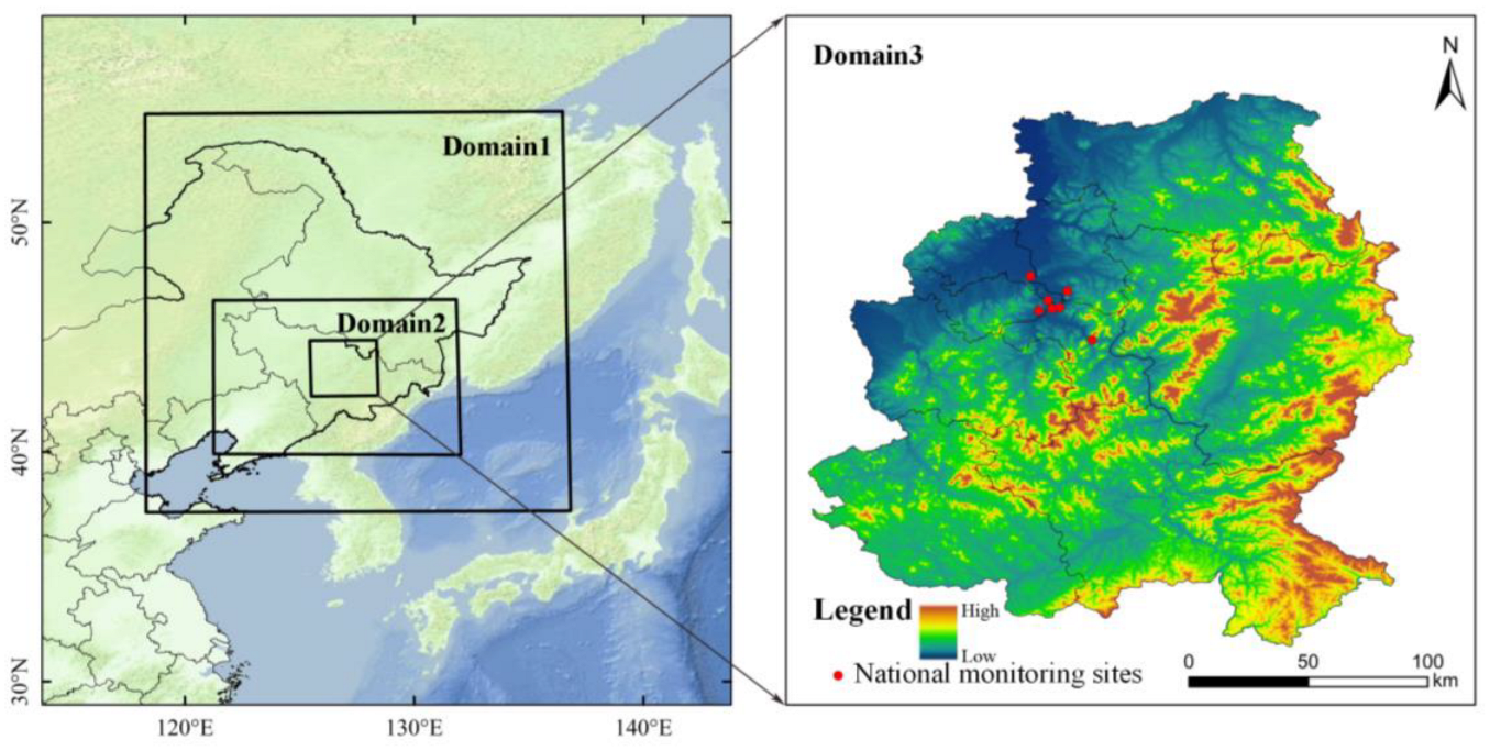
2.1. Overview of the Study Area

Jilin City, commonly referred to as “Beiguo River City”, is a prefecture-level city located in Jilin Province, northeastern China. Covering an area of 17,200 square kilometers, it is one of the primary cities in the province. Recognized by the State Council, Jilin City is a key industrial center, integral to the old industrial base of Northeast China, and an emerging industrial hub within Jilin Province. Geographically, it is situated between latitudes 42°31′ N and 44°40′ N and longitudes 125°40′ E and 127°56′ E, with a registered population of approximately 4.116 million, as of the end of 2020 [18].
Jilin City administers four districts and five county-level cities: Changyi District, Chuanying District, Fengman District, Longtan District, Shulan City, Panshi City, Jiaohe City, Huadian City, Yongji County. It borders Harbin to the north, Yanbian to the east, Changchun and Siping to the west, and Baishan, Tonghua, and Liaoyuan to the south. Geographically, the city is elevated in the southeast and lower in the northwest, bordered by mountains on one side and rivers on three sides. This topography results in a dry and warm climate during spring and autumn, accompanied by cold and prolonged winters. The precipitation in the city is mainly in the form of rainfall and snowfall, and the precipitation in the four seasons shows different characteristics, with the precipitation increasing significantly in winter and summer, while the precipitation in spring and autumn is less obvious. The city’s complex climate leads to highly uneven temperature distribution, with warmer temperatures generally observed in the west and northwest. The overall climate is characterized by low temperatures, with an average high temperature of 13 °C and an average low temperature of −1 °C in 2022, with the highest average temperature in July, an extreme high temperature of 33 °C on 26 July, the lowest average temperature in January, and an extreme low temperature of −28 °C on 13 January.

2.2. Data Sources

This study obtained air pollutant concentrations data from the National City Air Quality Real-Time Publishing Platform of the Ecological Environment Bureau (https://air.cnemc.cn:18007/, accessed on 5 July 2022). Meteorological data were sourced from the China Meteorological Data Service Center (http://data.cma.cn, accessed on 5 July 2022). We collected observational data from seven air quality monitoring stations and one meteorological station in Jilin City (Table S1). The air quality monitoring network consists of one background station in Fengman (FM) and six urban stations: Hada Bay (HDW), East Bureau (DJZ), Electric Power College (DJXY), Jiangbei (JB), Jiangnan Park (JNGY), and Nine Stations (JZ). Ozone concentrations (O3-8H) were recorded using an eight-hour sliding average, while CO, SO2, NO2, PM2.5, and PM10 concentrations were monitored hourly. Additionally, meteorological variables, including air pressure, wind speed, wind direction, and temperature, were recorded at meteorological stations across the country.
The emission inventory in this study is based on the China Multiresolution Emission Inventory, developed by the research team at Tsinghua University [19,20] (MEIC, http://meicmodel.org/ accessed on 11 March 2022), with a spatial resolution of 0.25° × 0.25°. This inventory is recognized for its versatility and accuracy [21]. MEIC anthropogenic emissions are classified into five sectors: industrial, power, transportation, residential, and agricultural. The pollutants analyzed include SO2, NO2, PM2.5, CO, and volatile organic compounds (VOCs) covering the region from 70° E to 150° E and 10° N to 60° N. We employed the Inventory Spatial Allocation Tool (ISAT) to spatialize the emission inventory and input the resulting data into the Community Multi-Scale Air Quality (CMAQ) model for numerical simulations. Emissions were allocated based on population, GDP, and land use grid data sourced from the Resources and Environmental Sciences Data Center of the Chinese Academy of Sciences [22].

2.3. WRF-CMAQ-ISAM Model

This study employed the WRF model (version 4.3.3) and the CMAQ model (version 5.4) [23] to simulate Jilin City and its surrounding regions, both of which are widely employed for mesoscale numerical simulations [24]. The ISAM module, a label-tracking method used in source apportionment, was employed within the CMAQ model to trace pollutants. WRF was used to simulate meteorological conditions, with initial weather fields sourced from the FNL Global Reanalysis dataset (http://rda.ucar.edu/datasets/ds083.2, accessed on 5 July 2022) provided by the National Center for Environmental Prediction. This dataset has a spatial resolution of 1° × 1° and a temporal resolution of 6 h. Simulations were conducted across three nested domains, with the outermost domain providing initial and boundary conditions for the inner domains. The spatial resolutions of Domain 1, Domain 2, and Domain 3 were 27 km × 27 km, 9 km × 9 km, and 3 km × 3 km, respectively, covering Northeast China, Jilin Province, and Jilin City. The simulation domains are illustrated in Figure 1.

2.4. Research Methods

To visually illustrate the changes in air quality and pollution sources in Jilin City during the 2022 epidemic, the research period was divided into four stages based on the progression of the outbreak and corresponding prevention and control measures issued by the Jilin City People’s Government on its official website. On 3 March 2022, COVID-19 was circulating again in Jilin City, which reported its first local COVID-19 case and three asymptomatic infections. Following initial contact tracing, it became clear that the virus had spread within the city. To contain the outbreak, traffic control was enforced at all entry and exit points starting on 4 March, and public transport in urban and rural areas was temporarily suspended on 6 March. Key urban bus routes remained operational, while others were temporarily suspended. From 7 to 11 March, all government offices, businesses, and institutions suspended operations, major schools and kindergartens closed, and all commercial venues shut down. On 14 March, Jilin City reported 2601 new confirmed cases, including 18 asymptomatic infections that were reclassified as confirmed cases. The Jilin Provincial Government’s Information Office held a press conference on epidemic prevention and control, announcing measures to prevent further spread. Starting 14 March 2022, cross-provincial and cross-city travel was restricted, especially in Changchun and Jilin City. On 8 April, the Jilin City Epidemic Prevention Headquarters announced that the city had achieved its goal of eliminating community transmission. By 28 April, social control measures were gradually lifted, and the normal order of production and daily life was systematically restored. On 12 May, with no new local confirmed cases or asymptomatic infections, the government fully lifted the lockdown. Based on this timeline, the research period was divided into four stages: Stage 1 (3 February to 3 March), Stage 2 (4 March to 27 April), Stage 3 (28 April to 11 May), and Stage 4 (12 May to 31 May). The first stage represents the pre-containment period, the second is the strict containment phase, the third is the orderly recovery phase, and the fourth is the post-containment observation phase.
This research employs the WRF-CMAQ model to simulate air quality during the strict containment period (4 March to 27 April). Firstly, the WRF model is used to simulate the meteorological effect and verify it to ensure that the output results of the model can provide more accurate meteorological data for the subsequent CMAQ simulation, and then the CMAQ model is used to simulate and verify the O3 concentration in the study period to ensure that the model can accurately present the change trend of O3 concentration. The ISAM module is employed to analyze industrial and regional O3 sources. The same simulation was also conducted for the same period in 2019. The contribution of different O3 emission sources and the impact of shutdown on O3 concentration were quantified, allowing for a comparison of the pollutant sources. The impact of industrial shutdowns during the epidemic on O3 levels was then evaluated. In CMAQ version 5.4, the MCIP must begin after the WRF weather field output. To minimize the impact of initial conditions, the WRF simulation was initiated five days earlier.

3. Results and Discussion

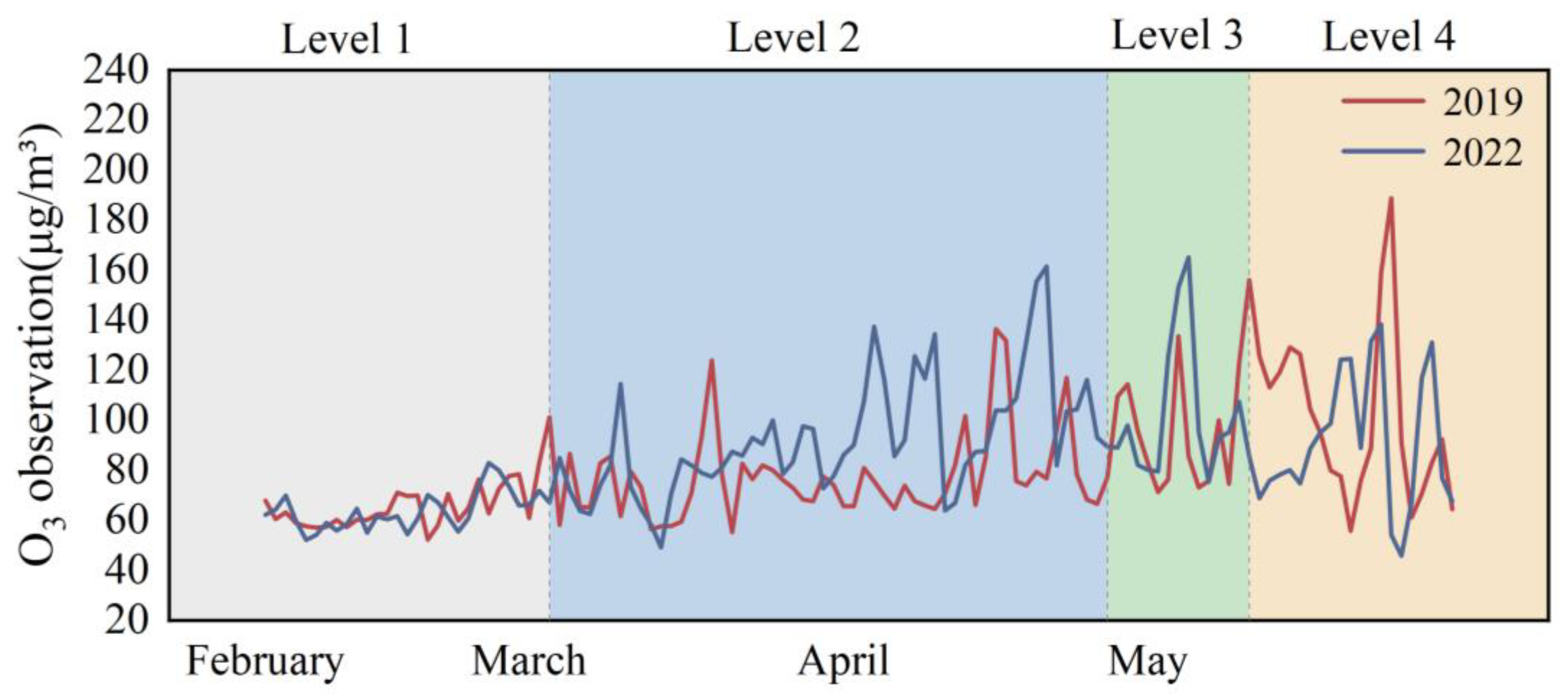
3.1. Analysis of Atmospheric O3 Concentrations

Although directly comparing O3 concentrations across different periods does not fully capture changes in regional O3 emissions, it still provides insight into long-term emission trends. To assess the impact of government measures on O3 concentrations during lockdown, we analyzed daily O3 concentration changes from 3 February to 31 May, 2019–2022. Figure 2 presents the daily and monthly average O3 concentrations during Levels 1 through 4 from 2019 to 2022, comparing O3 concentrations between 2019 (pre-epidemic) and 2022 (during the epidemic). In 2019, 2020, 2021, and 2022, the average concentration of O3 during Level 1 was 66.07 μg/m3, 70.47 μg/m3, 67.73 μg/m3, and 63.81 μg/m3, respectively. The average concentration of O3 during Level 2 was 77.25 μg/m3, 78.12 μg/m3, 75.05 μg/m3, and 92.21 μg/m3, respectively. The average concentration of O3 during Level 3 was 98.01 μg/m3, 90.17 μg/m3, 73.11 μg/m3, and 101.78 μg/m3, respectively. The average concentration of O3 during Level 4 was 100.09 μg/m3, 78.42 μg/m3, 90.53 μg/m3, and 91.41 μg/m3, respectively. During Level 1 in 2022, O3 concentrations were reduced by 3.42%, 9.45%, and 5.79% compared to the same period in 2019, 2020, and 2021, respectively. During Level 2 in 2022, O3 concentrations increased by 19.37%, 18.05%, and 22.87% compared to the same period in 2019, 2020, and 2021, respectively. During Level 3 in 2022, O3 concentrations increased by 3.84%, 12.88%, and 39.21% compared to the same period in 2019, 2020, and 2021, respectively. During Level 4 in 2022, O3 concentrations increased by −8.67%, 16.56%, and 0.97% compared to the same period in 2019, 2020, and 2021, respectively. Figure 3 compares O3 concentrations between 2019 and 2022. The remarkable increase in O3 concentrations is primarily due to a reduction in the titration reaction, which typically consumes O3 near the ground [25,26]. During the lockdown, restrictions on mobility and driving led to a significant reduction in vehicle exhaust emissions, which in turn reduced nitrogen oxide (NOx) concentrations [8]. This weakening of the titration reaction caused a notable increase in O3 concentrations compared to the same period in previous years.
Ozone-induced photochemical reactions can encompass thousands of species and more than 20,000 reactions. At present, the formation process of photochemical smog is usually summarized using a simplified mechanism composed of the following reactions [27,28].
(1)
Photochemical cycle of O3 with NO and NO2:
NO2 + hv (λ < 420 nm) → NO + O (3P)
O (3P) + O2 + M → O3
O3 + NO → NO2 + O2
(2)
Free radicals trigger a reaction:
O3 + hv (λ < 320 nm) → O (1D) + O2
O (1D) + H2O → OH + OH
HONO + hv (λ < 400 nm) → OH + NO
(3)
Free radical transport reactions:
CO + OH → H2O + CO2
VOCs + OH → RO2 + H2O
RCHO + OH → RC(O)O2 + H2O
RCHO + hy → RO2 + HO2 + CO
HO2 + NO → NO2 + OH
RO2 + NO → NO2 + RCHO + HO2
RC(O)O2 + NO → NO2 + RO2 + CO2
(4)
Free radical termination:
HO2 + HO2 + M → H2O2 + O2 + M
HO2 + RO2 → ROOH + O2
OH + NO2 + M → HNO3 + M
RC(O)O2 + NO2
Figure 4 illustrates the hourly O3 concentration trends across the four blockade stages. O3 concentration is lowest during Level 1, highest during Level 3, and peaks between 12:00 and 18:00. This peak occurs because temperatures are highest during this period, enhancing the photochemical reactions necessary for O3 formation. As temperatures rise, solar radiation intensifies, accelerating photochemical reactions and increasing O3 concentrations.

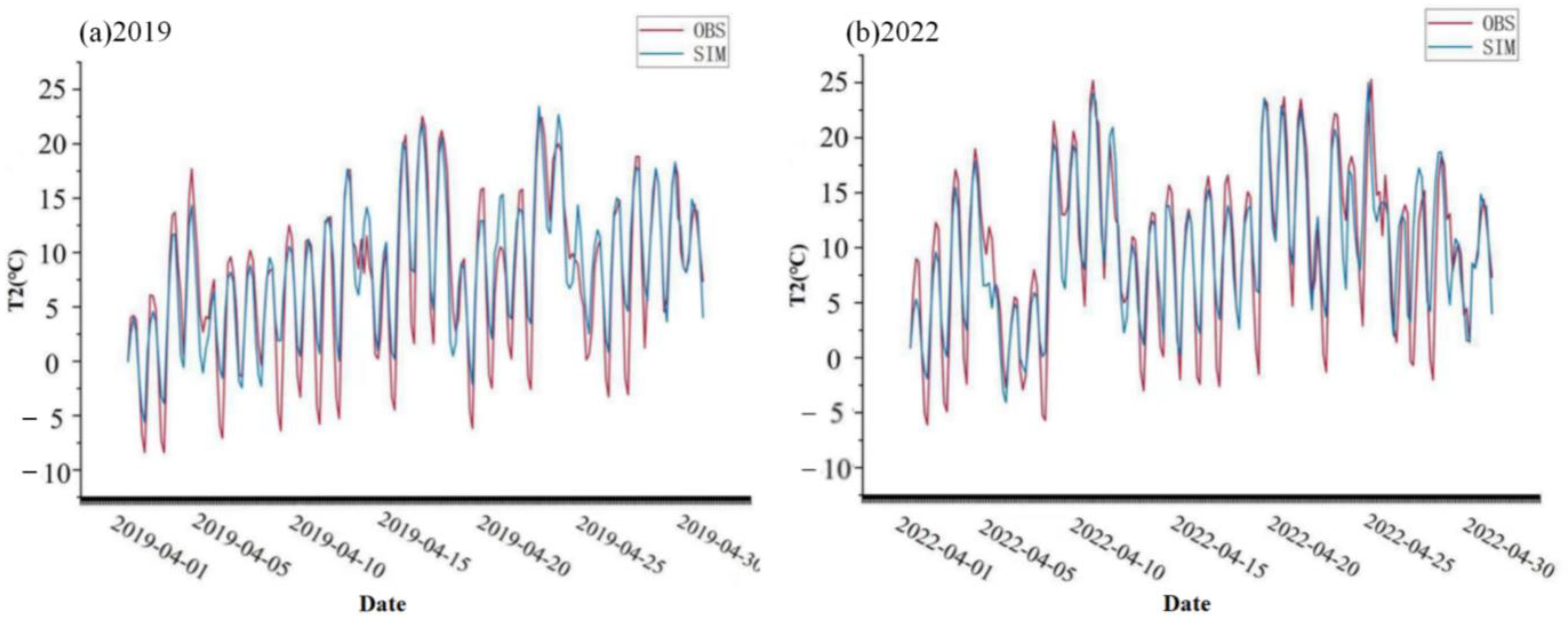
3.2. WRF Model Simulation Effect Evaluation

In addition to human activities and emission sources, meteorological conditions significantly influence the production, degradation, and transport of atmospheric pollutants, making their impact on air quality crucial. Adverse meteorological conditions can exacerbate air pollution and affect the accuracy of model simulation results [29]. Air pollution frequently correlates with meteorological changes. As surface temperatures rise, atmospheric molecules’ thermal movement increases, enhancing air mass convection. This process transports pollutants to higher altitudes, reducing surface concentrations. As wind speed and humidity increase, pollutants tend to diffuse, migrate, and transform horizontally, particularly during storms [30,31]. Seasonal variations also influence pollutant distribution. Severe pollution incidents are more likely in cold weather with low temperatures, while higher temperatures tend to correlate with lower pollutant concentrations. Severe weather conditions, such as haze, can exacerbate pollutant migration. Wind transports pollutants downwind, aiding local dispersion while also spreading them to other regions [32,33].
To evaluate the model’s performance, we verified and analyzed the simulation results for April 2019 and April 2022. The accuracy of the WRF model is essential for the reliability of the CMAQ model’s output. Therefore, we validated the monitoring data from Jilin City’s meteorological station by comparing it with WRF-simulated data. We selected the 2 m temperature (T2) and 10 m wind speed (WS10) for comparison. The statistical indicators used include linear correlation coefficient (R), normalized mean error (NME), normalized mean bias (NMB), and root mean square error (RMSE). NME quantifies the deviation between simulated and observed values, while NMB assesses the proximity of the simulation to the observations. A positive NMB indicates that the simulation overestimates the observed values, while a negative NMB indicates an underestimation. R represents the correlation between the simulation and observation trends, with a higher R indicating stronger correlation. RMSE assesses the magnitude of deviation between simulation and observation, with a smaller RMSE indicating less deviation.
The precise computational formulas for the four metrics are detailed as follows:
R = i = 1 N P i P ¯ O i O ¯ i = 1 N P i P ¯ 2 i = 1 N O i O ¯ 2
N M B = i = 1 N P i O i i = 1 N O i
N M E = i = 1 N P i O i i = 1 N O i
R M S E = i = 1 N O i P i 2 N
where N represents the total number of samples, Pi is the simulation result at moment i, Oi is the monitoring result at moment i, P ¯ is the average of the simulation results, and O ¯ is the average of the monitoring results.
The simulation results are output every 6 h, and the observations are also verified using the data recorded every 6 h. The results are shown in Figure 5 and Figure 6 and Table 1; the simulated meteorological values closely align with the observed values, demonstrating the model’s strong performance. So, in the calculation, N is 124 in March and 120 in April. The T2 simulation performs well, with R-values ranging from 0.88 to 0.92, passing the 0.01 significance level test, which indicates a strong correlation between simulated and observed values. The NMB ranges from 0.0002 to 0.08, and the NME ranges from 0.26 to 0.30, indicating that the simulated values slightly overestimate the observed values but remain closely aligned. The RMSE ranges from 2.91 to 3.35 °C. The R-value for WS10 ranges from 0.56 to 0.62, passing the 0.01 significance level test, suggesting a moderate correlation between the simulated and observed values. The NMB values range from 0.44 to 0.46, and the NME is 0.62, indicating that the simulated values overestimate but are reasonably close to the observed values. The RMSE ranges from 2.27 to 2.71 m/s.
This indicates the successful simulation of meteorological elements, providing accurate data for subsequent CMAQ simulations.

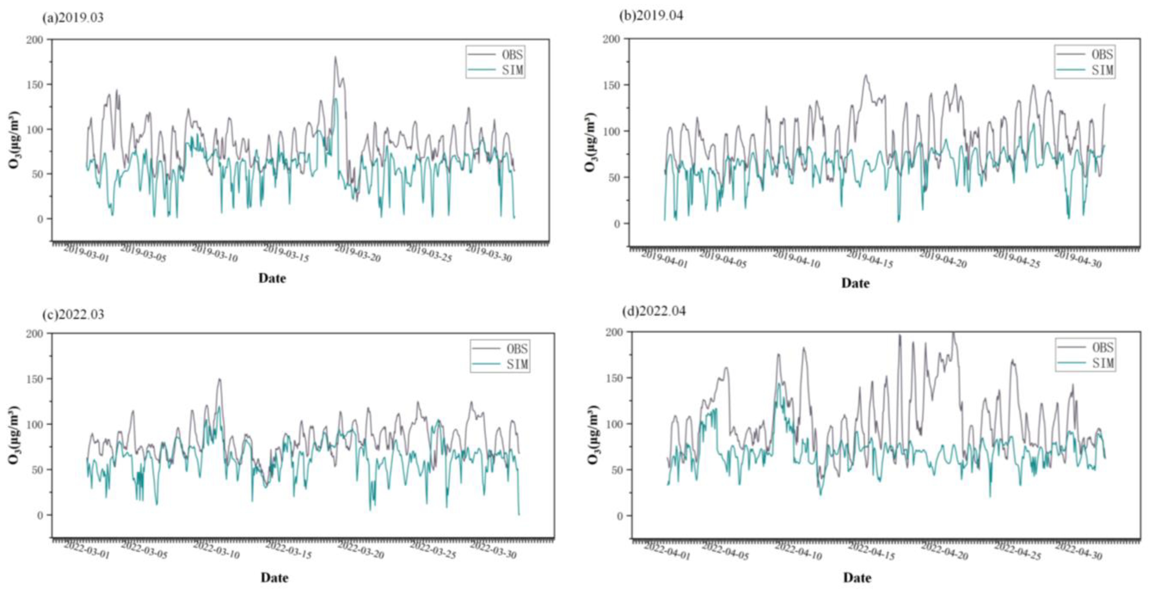
3.3. CMAQ Model Simulation Effect Evaluation

Given the varying terrain and meteorological conditions across different regions, along with uncertainties in emission sources, inventory accuracy, and model parameter settings, it is essential to evaluate the CMAQ model’s simulation results and assess its performance. This study focused on O3, comparing and analyzing simulated values from March and April of 2019 and 2022 against observed values from air quality monitoring stations. Statistical indicators, including the correlation coefficient (R), mean fractional bias (MFB), and mean fractional error (MFE), were employed. MFB and MFE are statistical metrics for assessing the performance of air quality models. Studies indicate that, when MFB is between −60% and 60%, and MFE is below 75%, the model’s simulation accuracy meets the required standards [34]. When MFB is between −30% and 30%, and MFE is under 50%, the model’s performance is considered better [35].
The precise computational formulas for the two metrics are detailed as follows:
M F B = 1 N i = 1 N P i O i ( O i + P i ) / 2
M F E = 1 N i = 1 N P i O i ( O i + P i ) / 2
where N represents the total number of samples, Pi is the simulation result at moment i, and Oi is the monitoring result at moment i.
As mentioned in 3.2, N is 124 in March and 120 in April. Table 2 shows the monthly averages of the simulated and observed data, as well as the statistical indicators. As shown in Table 2, the correlation coefficient (R) between simulated and observed O3 values over the four months ranges from 0.33 to 0.38. The mean fractional bias (MFB) for March and April 2019 and April 2022 falls below 60%, with MFE remaining under 75%, satisfying the criteria for model accuracy. For March 2022, the MFB is between −30% and 30%, and MFE is below 50%, indicating strong model performance. Figure 7 illustrates the temporal series of simulated and observed O3 values, revealing a close alignment between simulation trends and observation results. Overall, the CMAQ model developed in this study meets accuracy standards and effectively captures the trends in O3 concentrations.

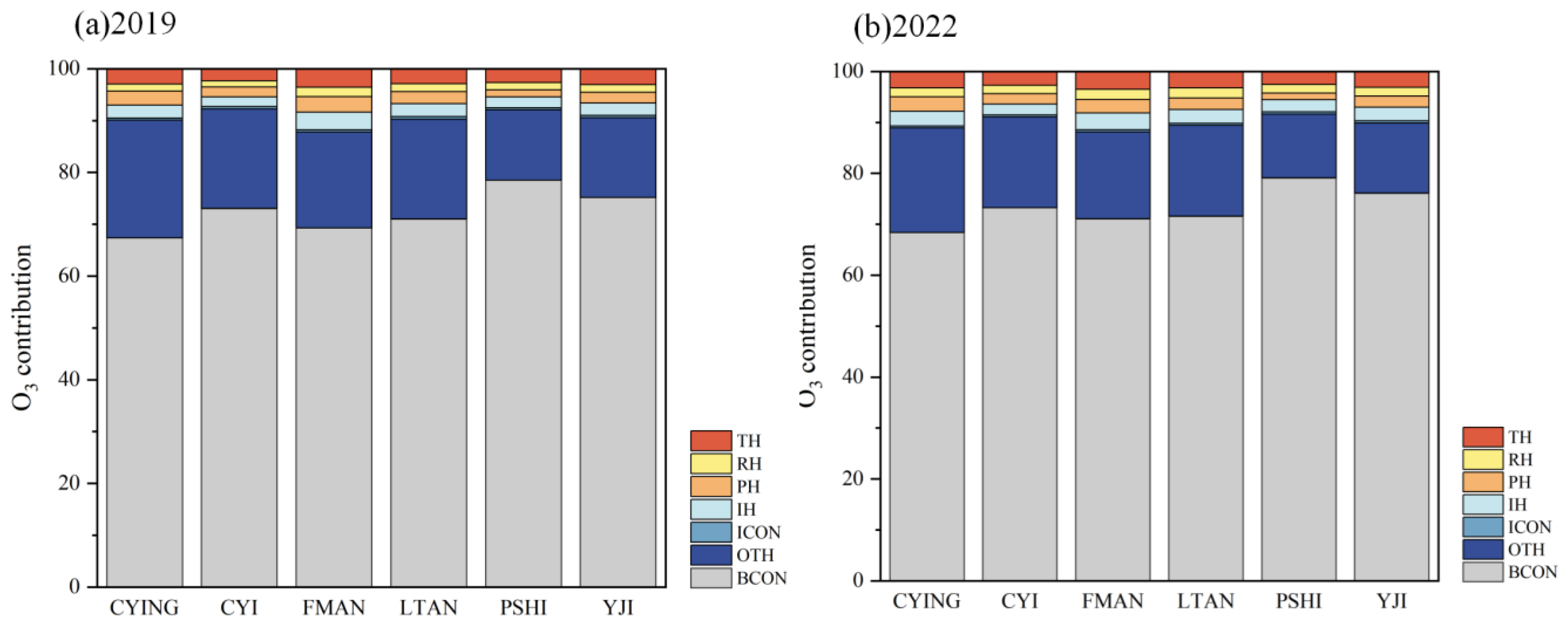
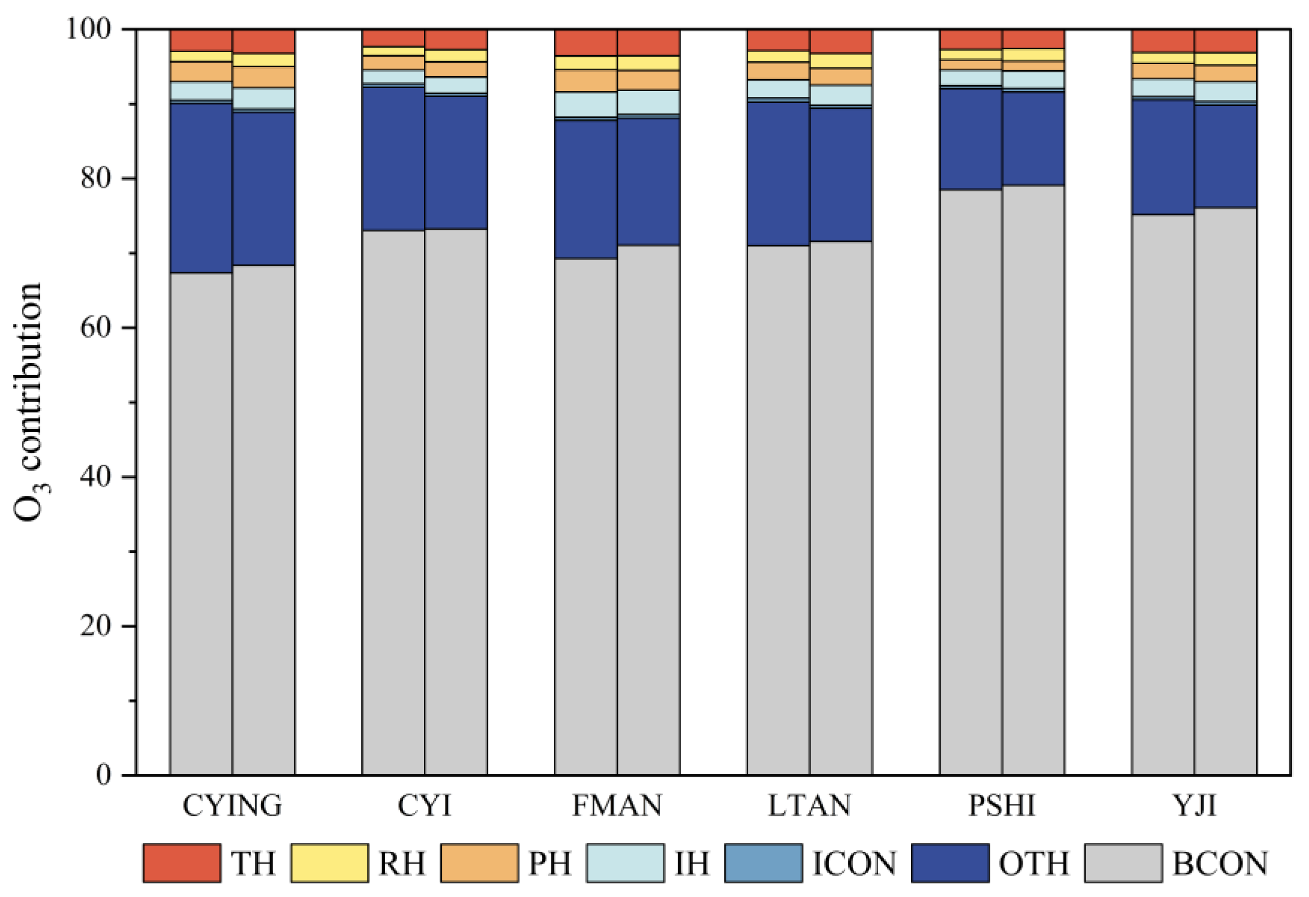
3.4. Analysis of Ozone Source Industry in Different Years

To assess the contribution of O3 emissions from different industries in Jilin City during the COVID-19 epidemic in 2022 compared to 2019, an analysis of O3 source characteristics by industry was conducted. This study utilized the ISAM source analysis tool in the CMAQ model to classify emission sources into IH (industrial), PH (power), RH (residential), and TH (traffic), with ICON (initial condition) and BCON (boundary condition) included in the emission inventory. Sources outside the simulation area were classified as OTH (other sources). Six districts in Jilin City were identified and labeled: CYING (Chuanying District), CYI (Changyi District), FMAN (Fengman District), LTAN (Longtan District), PSHI (Panshi City), and YJI (Yongji County). Refer to Figure S1 and Table S3 for labeling details. The statistical results in Table S4 indicate a significantly higher contribution from BCON compared to local industrial sources. In 2019, regional contribution rates ranged from 67.36% to 78.52%, with concentrations contributions between 33.562 and 45.277 µg/m3. Among industrial sources, TH made the highest contribution (2.31% to 3.57%), while RH had the lowest (1.22% to 1.83%). In 2022, the regional contribution rate increased to between 68.39% and 79.11%, with concentrations ranging from 36.67 to 48.82 µg/m3. Similarly, TH made the highest contribution (2.58% to 3.53%), while RH had the lowest (1.64% to 1.97%). Figure 8 illustrates the distribution of these sources in Jilin City, and Figure 9 shows the distribution characteristics of 2019 and 2022, concluding that traffic emissions are the primary direct contributor to local O3 levels, aside from boundary conditions and unclassified sources, with minimal variation in contributions across regions.
This study used the ISAM source analysis tool in the CMAQ model to classify emission sources into IH (industrial), PH (power), RH (residential), and TH (traffic), with ICON (initial condition) and BCON (boundary condition) noted in the emission inventory. Sources outside the simulation area were categorized as OTH (other sources). Six districts in Jilin City were identified and coded: CYING (Chuanying District), CYI (Changyi District), FMAN (Fengman District), LTAN (Longtan District), PSHI (Panshi City), and YJI (Yongji County). See Figure S1 and Table S3 for labeling details. The statistical results in Table S4 show a much higher contribution from BCON compared to local industrial sources. In 2019, regional contribution rates ranged from 67.36% to 78.52%, with concentrations contributions between 33.562 and 45.277 µg/m3. Among industrial sources, TH had the highest contribution (2.31% to 3.57%), while RH had the lowest (1.22% to 1.83%). In 2022, the regional contribution rate increased from 68.39% to 79.11%, with concentrations between 36.67 and 48.82 µg/m3. Similarly, TH had the highest contribution (2.58% to 3.53%), while RH had the lowest (1.64% to 1.97%). Figure 8 shows the distribution of these sources in Jilin City, concluding that traffic emissions are the main direct contributor to local O3 levels, aside from boundary conditions and unclassified sources, with little variation in contributions across regions.
Figure S2 illustrates the spatial distribution of emission concentration contributions from various industries in Jilin City for 2019 and 2022. The data indicate that O3 concentrations in 2022 are higher than in 2019, with traffic heating (TH) being the largest contributor and residential heating (RH) the smallest, consistent with previous research [36,37]. The figure illustrates severe O3 pollution in YJI and LTAN, with higher concentrations in suburban areas than in the urban core, confirming the conclusions of Tidblad et al. [38]. This can be attributed to limited vegetation in urban centers, where natural precursors from plants promote O3 formation, making suburban areas more susceptible to O3 pollution. O3 pollution in Jilin City exhibits regional characteristics, placing suburban and downwind residents at higher risk from elevated O3 levels.

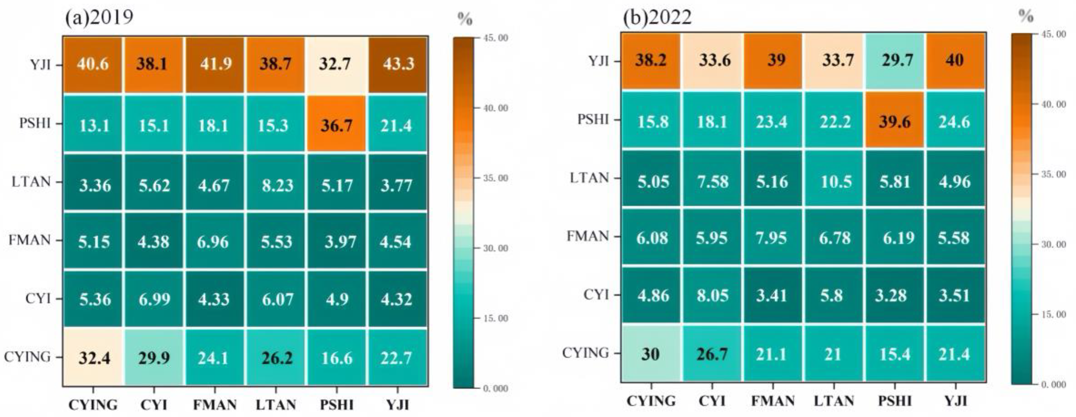
3.5. Analysis of Ozone Source Regions in Different Years

This study performed a quantitative simulation of O3 transmission contributions across six regions of Jilin City, comparing O3 source characteristics during the COVID-19 epidemic in 2022 with the same period in 2019. The transmission matrix refers to the source of O3 in each region of the simulation range. The results of the O3 source region analysis are presented in Table S5.
The results indicate that O3 concentrations in Jilin City are heavily influenced by long-distance transmission. In 2019, the BCON contribution ranged from 67.36% to 78.52%, while in 2022, it ranged from 68.39% to 79.11%, reflecting distinct regional transmission patterns. Previous studies have identified long-distance O3 transmission as a key factor in rising O3 concentrations [16]. BCON primarily transports NOx, VOCs, and other precursors from outside the inner simulation area to Jilin City over long distances. Additionally, stratospheric O3 descends and is easily transported by air masses, persisting for extended periods. Given that O3 formation takes time, BCON, which represents long-distance transmission, significantly contributes to total O3 levels [39]. The OTH contribution is largely associated with the effect of background methane on O3 within the inner simulation area, resulting in relatively uniform contributions across receptor regions: 13.52% to 22.72% in 2019 and 12.48% to 20.50% in 2022. ICON reflects the initial conditions, with contributions ranging from 0.41% to 0.52% in 2019 and from 0.39% to 0.49% in 2022, representing a minor proportion of the total.
In 2019, CYING’s contribution to other regions ranged from 1.25% to 2.84%, while CYI contributed between 0.37% and 0.51%, and FMAN’s contribution ranged from 0.30% to 0.51%. LTAN’s contribution ranged from 0.32% to 0.55%, PSHI contributed between 1.10% and 2.13%, and YJI’s contribution ranged from 2.47% to 4.93%. In 2022, CYING’s contribution to other regions ranged from 1.22% to 2.41%, while CYI contributed between 0.26% and 0.59%, and FMAN’s contribution ranged from 0.49% to 0.69%. LTAN’s contribution ranged from 0.46% to 0.65%, PSHI contributed between 1.55% and 2.68%, and YJI’s contribution ranged from 2.35% to 4.46%.
Figure 10 illustrates the transmission matrix of O3 contributions across various simulation regions in Jilin City, excluding ICON, BCON, and OTH. In the PSHI and YJI regions, local sources are the main contributors to O3 levels. Conversely, the other four regions are significantly influenced by long-distance transmission and sources from YJI. PSHI emerges as the primary local contributor to O3 emissions, accounting for 36.7% in 2019 and 39.6% in 2022. YJI is another significant local contributor, with 43.3% in 2019 and 40% in 2022. Furthermore, CYING, CYI, FMAN, and LTAN significantly contribute to O3 emissions in YJI, with contributions of 40.6%, 38.1%, 41.9%, and 38.7% in 2019, and 38.2%, 33.6%, 39%, and 33.7% in 2022, respectively.
There are significant disparities in the causes and sources of O3 pollution across various regions of Jilin City, along with notable interactions among these areas. YJI has the greatest influence on surrounding areas; however, this contribution is expected to decline during the lockdown period in 2022. This decrease is attributed to YJI’s role as the primary industrial hub in Jilin City, which promotes the development of a high-quality industrial economy. Industrial activity significantly decreased during the lockdown. To tackle future challenges of O3 pollution in Jilin City, implementing a regional collaborative prevention and control mechanism is essential.

4. Conclusions

This research analyzes O3 concentration trends in Jilin City during the COVID-19 lockdown of 2022, comparing them to O3 levels from the same period in 2019. The WRF-CMAQ model, combined with the ISAM module, was employed to assess industrial and regional contributions to O3 levels in Jilin City during the 2022 lockdown, in comparison to 2019.
Studies indicate a significant increase in O3 concentrations following the lockdown compared to before. This increase is attributed to decreased human activities, reduced traffic, and a significant decline in vehicle emissions. Consequently, NOx concentrations decline, weakening the titration process and decreasing O3 consumption near the surface. The findings also reveal significant long-range O3 transport in Jilin City, with BCON’s contribution slightly higher during the lockdown than in the non-lockdown period. Among the four industrial sources, transportation is the primary contributor to local O3 levels in Jilin City, with minimal variation in contributions across regions. This study identifies six districts in Jilin City, indicating that Panshi City and Yongji County are primarily influenced by local sources, while the other four districts are mainly affected by contributions from Yongji County. Yongji County’s contribution during the lockdown is slightly lower than in the non-lockdown period, as it serves as the main hub for industrial development in Jilin City.
Overall, the sources and causes of O3 pollution differ across various areas of Jilin City. These findings offer crucial insights for air quality management. Merely reducing anthropogenic NOx emissions is inadequate and may exacerbate O3 pollution; thus, controlling precursor emissions represents a more effective strategy. This analysis is also applicable to other countries and regions.
Future research will focus on analyzing the origins of O3 precursors in Jilin City and exploring variations in O3 sources across different regional transport pathways. Plans include collecting additional data, refining regional emission inventories, and employing a broader range of methodologies.

Supplementary Materials

The following supporting information can be downloaded at: https://www.mdpi.com/article/10.3390/atmos15111324/s1, Figure S1: ISAM marker area; Figure S2: Spatial distribution of O3 concentrations contribution from various industries in Jilin City; Table S1: List the 7 individual air quality monitoring sites and the 1 meteorological station; Table S2: WRF Physical process parameter scheme; Table S3: ISAM source resolution schema tag information; Table S4: O3 contribution statistics of various industries in Jilin City; Table S5: O3 regional transmission matrix of Jilin City.

Author Contributions

Conceptualization, S.Z. and J.W.; Data curation, C.F. and S.Z.; Formal analysis, S.Z. and X.Z.; Investigation, S.Z.; Methodology, C.F., S.Z. and X.Z.; Supervision, C.F.; Visualization, C.F., S.Z. and X.Z.; Writing—original draft, S.Z.; Writing—review and editing, C.F. and J.W. All authors have read and agreed to the published version of the manuscript.

Funding

Supported by Graduate Innovation Fund of Jilin University.

Institutional Review Board Statement

Not applicable.

Informed Consent Statement

Not applicable.

Data Availability Statement

The original contributions presented in the study are included in the article/Supplementary Materials; further inquiries can be directed to the corresponding author/s.

Acknowledgments

The authors would like to thank the group members of Laboratory 537 and 142 of Jilin University for their help and guidance for this study. Additionally, the authors would like to thank the MEIC team from Tsinghua University for providing the Multiscale Emission Inventory of China (MEIC).

Conflicts of Interest

The authors declare that they have no known competing financial interests or personal relationships that could have appeared to influence the work reported in this paper.

References

  1. Boogaard, H.; Walker, K.; Cohen, A.J. Air pollution: The emergence of a major global health risk factor. Int. Health 2019, 11, 417–421. [Google Scholar] [CrossRef] [PubMed]
  2. Chen, M.; Meng, J.; Li, Y.; Wang, Y.; Huang, T.; Li, Z.; Song, X.; Wu, C.; Hou, Z. Effect of COVID-19 lockdown on the characterization and mixing state of carbonaceous particles in the urban atmosphere of Liaocheng, the North China Plain. Particuology 2022, 78, 23–34. [Google Scholar] [CrossRef]
  3. Lonergan, M.; Chalmers, J.D. Estimates of the ongoing need for social distancing and control measures post-“lockdown” from trajectories of COVID-19 cases and mortality. Eur. Respir. J. 2020, 56, 2001483. [Google Scholar] [CrossRef] [PubMed]
  4. Impact Evaluation of COVID-19 Pandemic on Environmental Attributes; Maharashtra Pollution Control Board: Maharashtra, India, 2020.
  5. Tang, B.; Wang, X.; Li, Q.; Bragazzi, N.L.; Tang, S.; Xiao, Y.; Wu, J. Estimation of the Transmission Risk of the 2019-nCoV and Its Implication for Public Health Interventions. J. Clin. Med. 2020, 9, 462. [Google Scholar] [CrossRef]
  6. Hu, C.; Griffis, T.J.; Xia, L.; Xiao, W.; Liu, C.; Xiao, Q.; Huang, X.; Yang, Y.; Zhang, L.; Hou, B. Anthropogenic CO(2) emission reduction during the COVID-19 pandemic in Nanchang City, China. Environ. Pollut. 2022, 309, 119767. [Google Scholar] [CrossRef] [PubMed]
  7. Nie, D.; Shen, F.; Wang, J.; Ma, X.; Li, Z.; Ge, P.; Ou, Y.; Jiang, Y.; Chen, M.; Chen, M.; et al. Changes of air quality and its associated health and economic burden in 31 provincial capital cities in China during COVID-19 pandemic. Atmos. Res. 2021, 249, 105328. [Google Scholar] [CrossRef]
  8. Wang, J.; Shi, W.; Xue, K.; Wu, T.; Fang, C. Analysis of the Impact of Meteorological Factors on Ambient Air Quality during the COVID-19 Lockdown in Jilin City in 2022. Atmosphere 2023, 14, 400. [Google Scholar] [CrossRef]
  9. Bi, Z.; Ye, Z.; He, C.; Li, Y. Analysis of the meteorological factors affecting the short-term increase in O(3) concentrations in nine global cities during COVID-19. Atmos. Pollut. Res. 2022, 13, 101523. [Google Scholar] [CrossRef]
  10. Sicard, P.; De Marco, A.; Agathokleous, E.; Feng, Z.; Xu, X.; Paoletti, E.; Rodriguez, J.J.D.; Calatayud, V. Amplified ozone pollution in cities during the COVID-19 lockdown. Sci. Total Environ. 2020, 735, 139542. [Google Scholar] [CrossRef]
  11. Dunker.; Alan, M. Comparison of source apportionment and source sensitivity of ozone in a three-dimensional air quality model. Environ. Sci. Technol. 2002, 36, 2953–2964. [Google Scholar] [CrossRef]
  12. Li, Y.; Lau, A.K.H.; Fung, J.C.H.; Zheng, J.Y.; Zhong, L.J.; Louie, P.K.K. Ozone source apportionment (OSAT) to differentiate local regional and super-regional source contributions in the Pearl River Delta region, China. J. Geophys. Res. Atmos. 2012, 117, D15305. [Google Scholar] [CrossRef]
  13. Valverde, V.; Pay, M.T.; Baldasano, J.M. Ozone attributed to Madrid and Barcelona on-road transport emissions: Characterization of plume dynamics over the Iberian Peninsula. Sci. Total Environ. 2016, 543, 670–682. [Google Scholar] [CrossRef] [PubMed]
  14. Kwok, R.H.F.; Baker, K.R.; Napelenok, S.L.; Tonnesen, G.S. Photochemical grid model implementation and application of VOC, NOx, and O3; source apportionment. Geosci. Model Dev. 2015, 8, 99–114. [Google Scholar] [CrossRef]
  15. Yang, X.; Yang, T.; Lu, Y.; Jiang, M.; Zhang, S.; Shao, P.; Yuan, L.; Wang, C.; Wang, L. Assessment of summertime ozone formation in the Sichuan Basin, southwestern China. Front. Ecol. Evol. 2022, 10, 931662. [Google Scholar] [CrossRef]
  16. Collet, S.; Kidokoro, T.; Karamchandani, P.; Jung, J.; Shah, T. Future year ozone source attribution modeling study using CMAQ-ISAM. J. Air Waste Manag. Assoc. 2018, 68, 1239–1247. [Google Scholar] [CrossRef]
  17. Liu, H.; Zhang, M.; Han, X.; Li, J.; Chen, L. Episode analysis of regional contributions to tropospheric ozone in Beijing using a regional air quality model. Atmos. Environ. 2019, 199, 299–312. [Google Scholar] [CrossRef]
  18. Statistical Bulletin of National Economic and Social Development of Jilin City in 2021. Available online: http://tjj.jl.gov.cn/tjsj/tjgb/ndgb/202208/t20220801_8528331.html (accessed on 15 May 2024).
  19. Gao, L.; Liu, Z.; Chen, D.; Yan, P.; Zhang, Y.; Hu, H.; Liang, H.; Liang, X. GPS-ZTD data assimilation and its impact on wintertime haze prediction over North China Plain using WRF 3DVAR and CMAQ modeling system. Environ. Sci. Pollut. Res. Int. 2021, 28, 68523–68538. [Google Scholar] [CrossRef]
  20. Emery, C.; Liu, Z.; Russell, A.G.; Odman, M.T.; Yarwood, G.; Kumar, N. Recommendations on statistics and benchmarks to assess photochemical model performance. J. Air Waste Manag. Assoc. 2017, 67, 582–598. [Google Scholar] [CrossRef]
  21. Li, M.; Liu, H.; Geng, G.; Hong, C.; Liu, F.; Song, Y.; Tong, D.; Zheng, B.; Cui, H.; Man, H.; et al. Anthropogenic emission inventories in China: A review. Natl. Sci. Rev. 2017, 4, 834–866. [Google Scholar] [CrossRef]
  22. Wang, K.; Gao, C.; Wu, K.; Liu, K.; Wang, H.; Dan, M.; Ji, X.; Tong, Q. ISAT v2.0: An integrated tool for nested-domain configurations and model-ready emission inventories for WRF-AQM. Geosci. Model Dev. 2023, 16, 1961–1973. [Google Scholar] [CrossRef]
  23. Tesche, T.W.; Morris, R.; Tonnesen, G.; McNally, D.; Boylan, J.; Brewer, P. CMAQ/CAMx annual 2002 performance evaluation over the eastern US. Atmos. Environ. 2006, 40, 4906–4919. [Google Scholar] [CrossRef]
  24. Appel, K.W.; Bash, J.O.; Fahey, K.M.; Foley, K.M.; Gilliam, R.C.; Hogrefe, C.; Hutzell, W.T.; Kang, D.; Mathur, R.; Murphy, B.N.; et al. The Community Multiscale Air Quality (CMAQ) model versions 5.3 and 5.3.1: System updates and evaluation. Geosci. Model Dev. 2021, 14, 2867–2897. [Google Scholar] [CrossRef]
  25. Wang, T.; Xue, L.; Brimblecombe, P.; Lam, Y.F.; Li, L.; Zhang, L. Ozone pollution in China: A review of concentrations, meteorological influences, chemical precursors, and effects. Sci. Total Environ. 2017, 575, 1582–1596. [Google Scholar] [CrossRef]
  26. Cheng, N.; Li, R.; Xu, C.; Chen, Z.; Chen, D.; Meng, F.; Cheng, B.; Ma, Z.; Zhuang, Y.; He, B.; et al. Ground ozone variations at an urban and a rural station in Beijing from 2006 to 2017: Trend, meteorological influences and formation regimes. J. Clean. Prod. 2019, 235, 11–20. [Google Scholar] [CrossRef]
  27. Chameides, W.L.; Demerjian, K.L.; Albritton, D.; Amar, P.; Schultz, L. An Assessment of Tropospheric Ozone Pollution: A North American Perspective. 2000. Available online: https://www.epri.com/research/products/000000000001000040 (accessed on 15 May 2024).
  28. He, C.; Yang, L.; Cai, B.; Ruan, Q.; Hong, S.; Wang, Z. Impacts of the COVID-19 event on the NOx emissions of key polluting enterprises in China. Appl. Energy 2021, 281, 116042. [Google Scholar] [CrossRef]
  29. Zhang, H.; Wang, Y.; Hu, J.; Ying, Q.; Hu, X.M. Relationships between meteorological parameters and criteria air pollutants in three megacities in China. Environ. Res. 2015, 140, 242–254. [Google Scholar] [CrossRef]
  30. Li, J.; Duan, L.; Zhang, T. Analysis of Spatio-temporal Distribution Characteristics and Influencing Factors of PM2.5 and PM10 in Chinese Cities. Environ. Sci. 2024, 45, 1938–1949. [Google Scholar]
  31. Miao, L.; Liao, X.; Wang, Y. Diurnal Variation of PM2.5 Mass Concentration in Beijing and Influence of Meteorological Factors Based on Long Term Date. Environ. Sci. 2016, 37, 2836–2846. [Google Scholar]
  32. Zhao, C.; Wang, Y.; Wang, Y.; Zhang, H.; Zhao, B. Temporal and Spatial Distribution of PM2.5 and PM10 Pollution Status and the Correlation of Particulate Matters and Meteorological Factors During Winter and Spring in Beijing. Environ. Sci. 2014, 35, 418–427. [Google Scholar]
  33. Nie, S.; Wang, S.; Cui, J.; Liu, D.; Chen, J.; Tian, L.; He, B.; Shen, M. Spatio-Temporal Characteristics and Potential Source Areas of Seasonal Atmospheric Pollution in Shijiazhuang. Environ. Sci. 2021, 42, 5131–5142. [Google Scholar]
  34. Eder, B.; Yu, S. A performance evaluation of the 2004 release of Models-3 CMAQ. Atmos. Environ. 2006, 40, 4811–4824. [Google Scholar] [CrossRef]
  35. Ghazvini, M.V.; Ashrafi, K.; Shafiepour Motlagh, M.; Pardakhti, A.; Ghader, S.; Holsen, T.M. Simulation of atmospheric mercury dispersion and deposition in Tehran city. Air Qual. Atmos. Health 2020, 13, 529–541. [Google Scholar] [CrossRef]
  36. Xian, Y.; Zhang, Y.; Liu, Z.; Wang, H.; Wang, J.; Tang, C. Source apportionment and formation of warm season ozone pollution in Chengdu based on CMAQ-ISAM. Urban Clim. 2024, 56, 102017. [Google Scholar] [CrossRef]
  37. Shu, Q.; Napelenok, S.; Hutzell, W.T.; Baker, K.R.; Henderson, B.H.; Murphy, B.N.; Hogrefe, C. Comparison of ozone formation attribution techniques in the northeastern United States. Geosci. Model Dev. 2023, 16, 2303–2322. [Google Scholar] [CrossRef]
  38. Tidblad, J.; Mikhailov, A.A.; Henrikse, J. Improved Prediction of Ozone Levels in Urbanand Rural Atmospheres. Prot. Met. 2004, 40, 67–76. [Google Scholar] [CrossRef]
  39. Luo, Y.; Zhao, T.; Meng, K.; Hu, J.; Yang, Q.; Bai, Y.; Yang, K.; Fu, W.; Tan, C.; Zhang, Y.; et al. A mechanism of stratospheric O3 intrusion into the atmospheric environment: A case study of the North China Plain. Atmos. Chem. Phys. 2024, 24, 7013–7026. [Google Scholar] [CrossRef]
Figure 1. Simulation domains established for WRF model.
Atmosphere 15 01324 g001
Figure 2. Variation of daily average O3 observations from February to May for years (a) 2019, (b) 2020, (c) 2021, (d) 2022. (The different background color in panel a–d represents corresponding periods as labeled; the black dashed lines represent monthly average).
Atmosphere 15 01324 g002
Figure 3. Comparison of O3 observations in different years (2019 and 2022) at the same period. (The different background color in the panel represents corresponding periods as labeled).
Atmosphere 15 01324 g003
Figure 4. Hourly changes in O3 observations in different control periods.
Atmosphere 15 01324 g004
Figure 5. Comparison between T2 simulation results and observation results of the meteorological station. (a) 2019 and (b) 2022.
Atmosphere 15 01324 g005
Figure 6. Comparison between WS10 simulation results and observation results of the meteorological station. (a) 2019 and (b) 2022.
Atmosphere 15 01324 g006
Figure 7. Comparison between O3 simulation results and observation results. (a) March 2019, (b) April 2019, (c) March 2022 and (d)April 2022.
Atmosphere 15 01324 g007
Figure 8. Distribution of O3 contribution from emission sources in Jilin City (IH (industrial), PH (power), RH (residential), TH (traffic), ICON (initial condition), BCON (boundary condition), OTH (other sources), CYING (Chuanying District), CYI (Changyi District), FMAN (Fengman District), LTAN (Longtan District), PSHI (Panshi City), and YJI (Yongji County)). (a) 2019 and (b) 2022.
Atmosphere 15 01324 g008
Figure 9. Comparison of O3 contribution distribution of emission sources in Jilin City in 2019 and 2022; 2019 on the left and 2022 on the right (IH (industrial), PH (power), RH (residential), TH (traffic), ICON (initial condition), BCON (boundary condition), OTH (other sources), CYING (Chuanying District), CYI (Changyi District), FMAN (Fengman District), LTAN (Longtan District), PSHI (Panshi City), and YJI (Yongji County)).
Atmosphere 15 01324 g009
Figure 10. O3 regional transmission matrix diagram of Jilin City. (CYING (Chuanying District), CYI (Changyi District), FMAN (Fengman District), LTAN (Longtan District), PSHI (Panshi City), and YJI (Yongji County)). (a) 2019 and (b) 2022.
Atmosphere 15 01324 g010
Table 1. Statistical analysis of T2 and WS10 simulation results and observation results of the meteorological station.
MonthElementNMBNMERRMSE
April 2019T2 (°C)0.080.300.92 **2.91
WS10 (m/s)0.460.620.62 **2.27
April 2022T2 (°C)0.00020.260.88 **3.35
WS10 (m/s)0.440.620.56 **2.71
** There was a significant association at 0.01 level (bilateral).
Table 2. Statistical analysis of O3 simulation results and observation results.
March 2019April 2019March 2022April 2022
Simulation value (μg/m3)48.1553.5662.5769.55
Observation value (μg/m3)83.7792.6282.49104.09
R0.36 **0.38 **0.34 **0.33 **
MFB−41.11%−37.45%−29.32%−35.99%
MFE44.42%42.19%33.37%39.63%
** There was a significant association at 0.01 level (bilateral).
Disclaimer/Publisher’s Note: The statements, opinions and data contained in all publications are solely those of the individual author(s) and contributor(s) and not of MDPI and/or the editor(s). MDPI and/or the editor(s) disclaim responsibility for any injury to people or property resulting from any ideas, methods, instructions or products referred to in the content.

