Influence of Model Resolution on Wind Energy Simulations over Tibetan Plateau Using CMIP6 HighResMIP

Abstract

The assessment of wind energy resources is critical for the transition from fossil fuel to renewable energy sources. Using the outputs from high-resolution global climate models (GCMs), such as the High Resolution Model Intercomparison Project (HighResMIP) of the Coupled Model Intercomparison Project Phase 6 (CMIP6), has become one of the most important tools in wind energy research. This study evaluated the reliability of the 22 GCMs available in the HighResMIP-PRIMAVERA project by simulating the wind energy climatology and variability over the Tibetan Plateau (TP) with reference to observations and investigated the differences in performance of the GCMs between high-resolution (HR) and low-resolution (LR) simulations. The results show that most models performed relatively well in simulating the probability distribution of the observed wind speed over the TP, but nearly half of the models generally underestimated the wind speed, whereas the others tended to overestimated the wind speed. Compared with the wind speed, the GCMs showed larger biases in reproducing the wind power density (WPD) and other wind energy resources, whereas the biases in multi-model ensembles were relatively smaller than those in most individual models. With respect to interannual variability, both the HR and LR models failed to capture interannual variations in WPD over the TP. Furthermore, more than half of the HR GCMs had a reduced bias relative to the corresponding LR GCMs, indicating the good performance of most HR models in simulating wind energy resources over the TP in terms of spatial pattern and temporal variability. However, the overall performance of HR GCMs varied among models, which suggests that solely improving the horizontal resolution is not sufficient to completely solve the uncertainties and deficiencies in the simulation of wind energy over complex terrain.

1. Introduction

Wind energy is widely recognized as one of the most crucial alternative and renewable clean energy sources worldwide and has been rapidly growing over the past few decades [1,2,3]. With the rapid development of technology, wind energy resources in many regions with complex terrains, such as mountains, basins, and slopes, have been widely developed in recent years [4,5].

The Tibetan Plateau (TP) is regarded as the largest (2.5 × 10⁶ km²) and highest (with an average altitude of 4000 m above sea level) plateau on earth, and it not only fundamentally influences the climate over East Asia but is also famous for its abundant wind energy resources. Rough statistics indicate that the total available wind energy across the TP amounts to a staggering 77.3 × 10¹⁰ kW [5]. In recent years, significant efforts have been made to harness the potential of clean energy on the TP, continuously advancing the construction of numerous clean energy projects. Notably, wind, solar, and other representatives of the clean energy industry have achieved remarkable progress. For example, a study showed that the Qaidam Basin, located in the northeastern part of the TP, boasts solar and wind energy potentials estimated at 5.7 trillion kWh and 0.9 trillion kWh annually, respectively, rendering it ideal for large-scale solar and wind energy development [6]. However, the wind energy over the TP strongly fluctuates and is extremely unstable because of its complex terrain [7]. Several studies have noted that the spatial and temporal distributions of wind speed over the TP and the trends of wind speed vary across seasons and regions, particularly over higher elevations in the TP [8,9]. Future projections also indicate that the TP will experience the most remarkable reduction in near-surface wind speed (SWS) in China, and the variability in wind energy over the TP is expected to increase under high-emission scenarios [10,11,12,13]. Although some studies have been carried out to assess the wind energy potential over the TP, accurate evaluations of the wind energy over the TP remain a great challenge for researchers and developers because of the rugged terrain and harsh weather and climate conditions around the TP.

Global climate models (GCMs) are an important tool for simulating atmospheric circulation and other critical aspects of the Earth’s climate system and are widely used in wind energy assessments, particularly for regions where in-situ observations are scarce. Numerous studies have employed GCMs to investigate the characteristics of wind speed and wind energy, as well as to project their future changes under various emission scenarios across different regions of the globe, including China [12], the Indian Ocean https://esgf-node.llnl.gov [14], West Africa [15,16], Europe [17], and North America [18]. Given the inherent uncertainties in climate simulations, several studies have adopted multi-model ensembles (MMEs) or bias correction methods to estimate historical wind energy and project future changes [19,20,21,22,23]. However, the capability of GCMs in simulating past, present, and future meteorological variables is closely tied to their dynamic framework, boundary conditions, and physical parameterization schemes, with a particular sensitivity to the horizontal resolution of the models, as highlighted by previous studies [24,25]. To address this limitation, the sixth phase of the Coupled Model Intercomparison Program (CMIP6) High Resolution Model Intercomparison Project (HighResMIP) protocol aims to systematically evaluate and compare the influences of different spatial resolutions on model simulations. It further provides free multi-model and multi-resolution outputs to the global research community [22,26]. This initiative offers a valuable opportunity to increase the accuracy and reliability of GCM-based wind energy assessments and projections.

Under the HighResMIP protocol, the Process-Based Climate Simulation: Advances in High-Resolution Modelling and European Climate Risk Assessment (PRIMAVERA) project, funded by the European Union Horizon 2020 program, has conducted GCMs simulations at various resolutions, specifically at approximately 100 km and 25 km. These simulations enable us to conduct a more thorough investigation into wind energy over the TP and to scrutinize the impact of lower resolution (LR) and higher resolution (HR) on the model’s ability to simulate wind energy over the region [26]. HighResMIP is a pivotal component of CMIP6, specifically designed to evaluate the effects of increased horizontal resolution in GCMs on the simulation of climate processes [26]. This project offers a coordinated framework for conducting high-resolution modeling experiments, enabling comparisons across various models and resolutions. Its core objective is to deepen our understanding of how model resolution affects the representation of climate variability and extremes, which is critical for regional climate studies and impact assessments [27]. Applications of HighResMIP simulations span diverse research fields, including extreme weather events, hydrological cycles, and regional climate variability [10]. However, studies specifically dedicated to wind energy assessments, particularly in complex terrains such as the TP, remain scarce.

Numerous studies have demonstrated that HR simulation outputs can substantially enhance the capability of GCMs to represent topographical features and their resultant impacts, thereby enabling more accurate reproductions of small- and medium-scale weather systems [28]. Furthermore, GCMs with finer resolutions tend to perform better in simulating large-scale atmospheric circulation and climate system changes, including phenomena such as the Atlantic meridional overturning Circulation [26], tropical cyclone precipitation [29], and global monsoon variability [30]. However, some research suggests that an increase in model resolution does not invariably result in significant improvements in the accuracy of weather and climate simulations [31]. While HighResMIP has successfully enhanced the simulation of atmospheric circulation and precipitation patterns, especially in rugged terrain [26], higher-resolution models do not uniformly offer superior descriptions of regional climate processes, such as wind speed and precipitation, across all variables and regions [27,31]. Addressing this inconsistency is crucial for model enhancement and ensuring accurate simulations and projections of wind energy. In this paper, we aim to evaluate the extent to which increased model resolution enhances the simulation of wind energy over the TP, a region characterized by its intricate terrain and substantial wind energy potential, by comparing the outputs of HR and LR GCMs. This study not only addresses a gap in the application of HighResMIP simulations to wind energy assessments in the TP but also provides new insights into the advantages and limitations of HR modeling in simulating wind energy resources. Our findings will offer new perspectives to both the climate modeling community and stakeholders in the wind energy sector, facilitating future model advancements and resource planning.

The rest of this paper is organized as follows: Section 2 provides a concise description of the data and methodologies employed in this study. Section 3 evaluates the performance of the CMIP6 HighResMIP models in simulating wind energy over the TP. Finally, Section 4 summarizes and discusses the key findings of this study.

2. Data and Methods

2.1. Observations and HighResMIP Simulations

Two datasets were employed in this study. The primary dataset consisted of daily SWS measurements at a height of 10 m, derived from the 0.25° × 0.25° gridded dataset of CN05.1. This dataset is derived from near-surface wind speed observations at 10 m from 2416 meteorological stations across China, developed by the National Climate Center of China, using an anomaly-based interpolation method (available at http://www.ncc-cma.net, accessed to 4 December 2023) [32]. This dataset is widely used in weather and climate change studies, because of its high spatiotemporal resolution and national coverage. To ensure a rigorous comparison of the discrepancies between the HR and LR simulations and observations, all the data were linearly interpolated to the gird box at a resolution of 0.5° × 0.5°. The simulated SWS at 10 m was sourced from the HighResMIP-PRIMAVERA project. Each model was executed with at least two distinct grid resolutions, namely, an HR simulation and an LR simulation. The information on the models utilized in this study is shown in

Table 1. Basic information about the GCMs used in this study.

Model Name	Institute	Horizontal Resolution Lat × Lon
CMCC-CM2-VHR4	CMCC	768 × 1152
CMCC-CM2-HR4		192 × 288
CNRM-CM6-1-HR	CNRM-CERFACS	360 × 720
CNRM-CM6-1		128 × 256
EC-Earth3P-HR	EC-Earth-Consortium	512 × 1024
EC-Earth3P		256 × 512
ECMWF-IFS-HR	ECMWF	361 × 720
ECMWF-IFS-LR		181 × 360
FGOALS-f3-H	CAS	720 × 1440
FGOALS-f3-L		180 × 288
HadGEM3-GC31-HM	MOHC	768 × 1024
HadGEM3-GC31-LM		144 × 192
HiRAM-SIT-HR	AS-RCEC	768 × 1536
HiRAM-SIT-LR		360 × 720
IPSL-CM6A-ATM-HR	IPSL	361 × 512
IPSL-CM6A-ATM-LR		143 × 144
MPI-ESM1-2-XR	MPI-M	384 × 768
MPI-ESM1-2-HR		192 × 384
MRI-AGCM3-2-S	MRI	960 × 1920
MRI-AGCM3-2-H		320 × 640
NICAM16-8S	MIROC	640 × 1280
NICAM16-7S		320 × 640

. Furthermore, all data for the model were selected from daily data for the period of 1950–2014. Detailed information about the models, including the institute, horizontal resolution, initialization processes, boundary conditions, and model setup, can be accessed at https://esgf-node.llnl.gov/search/cmip6, accessed to 4 December 2023.

2.2. Methods

Several wind energy indices and statistical methods, including the wind power density (WPD), effective wind hour (EWH), coefficient of variation (CV), index of agreement (IA), and interannual variability score (IVS), were employed to assess the impact of model resolution on wind power simulations over the TP. To make this paper more self-contained, the formulas for these wind energy indices and statistical methods are presented below.

The WPD is regarded as an important index for wind resource assessment and is calculated by:

$$WPD={\displaystyle \frac{1}{2}}{\rho }_h\cdot v_h^3,$$

(1)

where $v_h$ and ${\rho }_h$ are the wind speed and air density at the hub height of wind turbines, respectively.

The wind speed from the model simulations and CN05.1 at 10 m are extrapolated to the wind speed at 100 m via the power law since the typical hub height of a modern wind turbine can reach 100 m:

$$v_h=v_{10}\cdot {\left({\displaystyle \frac{Z_h}{Z_{10}}}\right)}^{\alpha },$$

(2)

where $v_h$ represents the wind speed at the height of h, $v_{10}$ represents the reference wind speed at 10 m, and α represents the wind shear index, which was set as equal to 1/7 [15].

The air density at the hub height of the wind turbines was calculated as follows:

$${\rho }_h={\rho }_0{\left(1-{\displaystyle \frac{HL}{T_0}}\right)}^{{\displaystyle \frac{gM}{RL}}-1},$$

(3)

where ${\rho }_0$ and T₀ are the standard air density (1.292 kg·m⁻³) and air temperature (288.15 K) at sea level, respectively, L is the temperature gradient (0.0065 K·m⁻¹), g is the Earth’s gravitational acceleration (9.80665 m·s⁻²), and M is the gas molar mass (0.0289652). Figure 1 shows the spatial distribution of the actual air density over the TP, according to Equation (3).

The EWH reflects the availability of wind energy, and its formula is:

$$EWH={\displaystyle \frac{t}{T}}\times 100\%,$$

(4)

where t is the accumulation of hours of wind speed between the cut-in (3 m·s⁻¹) and cut-out (20 m·s⁻¹) on the wind turbines, and T is the total number of hours during the study period [33].

Similar to a previous study [34], the CV was used to assess the stability of WPD over the TP:

$$CV={\displaystyle \frac{{\sigma }_{WPD}}{\overline{WPD}}},$$

(5)

in which ${\sigma }_{\mathrm{WPD}}$ is the standard deviation, and $\overline{\mathrm{WPD}}$ is the mean of WPD.

To estimate the performance of GCMs in reproducing the probability distribution of wind speed and the interannual variability in WPD, the IA and IVS were used, and their formulas are as follows:

$$IA=1-{\displaystyle \frac{{\displaystyle \sum _{i=1}^n{(O_i-M_i)}^2}}{{\displaystyle \sum _{i=1}^n{(|M_i-\overline{O}|+|O_i-\overline{O}|)}^2}}},$$

(6)

$$IVS={\displaystyle \sum _{i=1}^n{(\frac{{\sigma }_{Mi}}{{\sigma }_{Oi}}-\frac{{\sigma }_{Oi}}{{\sigma }_{Mi}})}^2},$$

(7)

where M_i and O_i represent simulations and observations, respectively, and $\sigma$ is the standard deviation.

To examine the agreement between the observations and simulations, the Taylor diagram was used to assess the simulated spatial patterns of EWH, WPD, and CV in comparison with those of CN05.1 [35]. Furthermore, our assessment was based on individual models and the MME of HR (HMME) and LR (LMME) outputs, which are widely used in climate research because they substantially reduce uncertainties among GCMs [36].

3. Results and Discussion

Figure 2 presents the climatic means of the observed and simulated (by both LR and HR) probability distributions of the wind speed at 100 m over the TP provided by 22 models from 11 institutes as well as their MME. For the observations, the maximum wind speed over the TP was 19.35 m·s⁻¹, and the probability distribution exhibited considerable skewness with a long tail toward the right-hand side. The wind speed value of 3.8 m/s was the peak probability of the observed wind speed, followed by the median (5.0 m·s⁻¹), and the mean (5.4 m·s⁻¹) had the lowest probability of the three measures. The cumulative probabilities of the observed wind speeds range from 12.96% for speeds of 0–3 m·s⁻¹ to 6.54% for speeds of 9–12 m·s⁻¹, with the breakdown as follows: 0–3 m·s⁻¹ (12.96%), 3–6 m·s⁻¹ (51.41%), 6–9 m·s⁻¹ (28.32%), and 9–12 m·s⁻¹ (6.54%). This distribution indicates that most of the observed wind speeds over the TP were less than 12 m·s⁻¹.

For the kurtosis coefficients of the probability curve of the simulated wind speed over the TP, nearly half of the models, including CNRM-CERFACS, EC-Earth-Consortium, ECMWF, MOHC, and AS-RCEC, exhibited significantly larger values than that of the observations. Furthermore, the simulated mode values of the wind speed were also lower than the observations, with ECMWF displaying the most pronounced “left-skewed” distribution, suggesting that these models underestimated the wind speed over the TP. In contrast, the mode values of the wind speed simulated by the MME, CMCC, CAS, MPI, MRI, and MIROC were larger than the observations, with the CMCC and CAS exhibiting a more “right-skewed” distribution, indicating an overestimation of the wind speed. In general, the cumulative probability statistics reveal that the probabilities of low and medium wind speeds (0–6 m·s⁻¹) simulated by the “right-skewed” models were somewhat lower than observations, whereas the probability of high wind speeds (>6 m·s⁻¹) was higher than that of the observation. Conversely, for the “left-skewed” models, the opposite trends could be observed. This indicates an improvement in the HR simulations of certain models of wind speed over the TP, though the degree and direction of improvement differed between models that overestimated and those that underestimated the observed values.

The IA can quantitatively assess the similarity between simulations and observations, with a value closer to 1.0 signifying a stronger agreement between the two groups. Figure 3 presents the IA values for the probability distributions of the HR and LR models. It is evident that the IPSL exhibited the highest IA, indicating the best agreement with the observations, whereas the ECMWF model yielded the lowest IA value, suggesting its poor performance in simulating the characteristics of wind speed over the TP. Furthermore, our analysis indicates that the LR versions of four models, including CNRM-CERFACS, EC-Earth-Consortium, CAS, and IPSL, generally outperformed their HR versions in representing the wind speed at 100 m over the TP. Conversely, the remaining HR verison models, particularly ECMWF, MOHC, and AS-RCES, showed superior performance compared with their LR outputs.

The EWH, an effective index in wind energy resource assessment, serves as a fundamental prerequisite for the selection of wind farm sites and turbine types while also ensuring the safe and efficient operation and maintenance of wind turbines. Figure 4 presents the spatial distributions of the observed and simulated EWH across the TP. The figure shows that the observed EWH over the TP exhibited a distinct southeast–northwest pattern gradient, with consistently high values (greater than or equal to 80%) in the central and northwestern regions and relatively low values (generally ranging from 40 to 60%) in the eastern and southeastern parts, indicating a staggered mosaic distribution. Compared with the observations, most of the models exhibited a certain ability to simulate the EWH over the TP, although there were variations in performance among individual models and between the LR and HR categories. Notably, models such as AS-RCEC, EC-Earth3P-Consortium, ECMWF, MOHC, and IPSL exhibited superior performance, with spatial patterns closely resembling those of the observations. However, in the western TP, models such as the CMCC, CAS, FGOALS, MPI, MRI, and NICAM showed significant deviations or biases from the observations and these biases in simulations may be attributed to the fact that there are substantial deficiencies of current GCMs for reproducing atmospheric and land processes over complex terrain regions.

Additionally, the MMEs (HMME and LMME) effectively ameliorated the underestimation of EWH in the western TP region by the models. Despite a deviation between the EWS presented by most models and the observed data, the HR offered more spatial detail than the LR did, reflecting an improvement in the ability of the HR models to simulate wind speeds over the complex terrain of the TP from another perspective. Regarding the difference between the HR and LR simulations, substantial biases were evident across most areas of the TP. However, an increase in model resolution partially reduced these biases in wind energy simulation, although this effect was not uniformly observed in all models. While the spatial patterns of EWH simulated by most HR models did not perfectly align with observations, the HR simulations exhibited clearer spatial detail compared with the LR models. This was likely due to the finer resolution of the HR models, suggesting a potential improvement in the simulation of EWH over the TP.

To quantitatively evaluate the performance of the GCMs in simulating the spatial distribution of EWH over the TP, the Taylor diagram was utilized. The statistical metrics, namely, spatial correlation correlation (SCC), spatial standard deviation (SSTD), centered root-mean-square error (CRMSE), and relative bias (RB), for both HR and LR simulations, are presented in Figure 5. Compared with the observations, all GCMs exhibited SCC values below 0.50, with CNRM-CM6-1-HR displaying the weakest correlation (r = 0.20), whereas HadGEM3-GC31-LM has the highest correlation (r = 0.53). With respect to the SD, most of the models presented values of less than 1.00, suggesting that the simulated spatial variability was lower than that observed. Compared with the reference EWH, the ECMWF exhibited a relatively good agreement in terms of variability. Conversely, MPI-ESM1-2-XR and HadGEM3-GC31-HM exhibited high variability relative to the observations. In terms of CRMSE, all the models fell within a range of 0.84 to 2.41. Notably, MPI-ESM1-2-XR exhibited the best ability in simulating the spatial pattern of EWH, with the smallest CRMSE value of 0.84. In contrast, the highest CRMSE value is achieved by CNRM-CM6-1-HR, indicating that it had the poorest performance compared with the other models. For the RB, the top five models in order of their performance were CNRM-CM6-1, IPSL-CM6A-ATM-HR, IPSL-CM6A-ATM-LR, NICAM16-7S, and MPI-ESM1-2-XR.

Figure 6 presents the observed and simulated climatic mean of the spatial distribution of WPD over the TP. The observed WPD clearly resembled that of the estimated EWH, exhibiting a distinct southeast-to-northwest gradient (Figure 6a). Specifically, regions in the northwestern TP exhibited WPD values exceeding 100 W·m⁻², with the maximum value reaching 427.73 W·m⁻². In contrast, the WPD was relatively lower in the eastern and southeastern parts of the TP, with some areas having values of less than 30 W·m⁻². Compared with the observations, most of the models, as well as the HMME and LMME, tended to underestimate the WPD, suggesting a limited ability to accurately reproduce the spatial distribution of WPD over the TP (Figure 6b–y).

The Taylor diagram for the HR- and LR- simulated and observed WPD over the TP is presented in Figure 7. Notably, simulations from CNRM-CERFACS, AS-RCEC, MRI and MIROC struggled to reproduce the spatial pattern of WPD over the TP. In contrast, ECMWF, MOHC, EC-Earth-Consortium, and the MME demonstrated relatively better agreement with the observations, with the SCCs of HR and LR being 0.58 (0.64), 0.62 (0.57), 0.57 (0.61), and 0.39 (0.49), respectively. In addition to the SCC, the SSTDs of the simulated WPD from the HR and LR models ranged from 0.32 to 2.65 and from 0.14 to 2.20, respectively, indicating significant differences in their ability to reproduce the spatial variability in WPD. Additionally, the CRMSEs for the HR simulations (0.81 to 2.51) and the LR simulations (0.82 to 2.53) further underscore these discrepancies. Among them, HadGEM3-GC31-HM (0.80), EC-Earth3P (0.81), and EC-Earth3P-HR (0.82) ranked as the top models in simulating the spatial pattern of WPD over the TP, whereas FGOALS-f3-H (2.04), MRI-AGCM3-2-H (2.14), and CMCC-CM2-VHR4 (2.53) were the poorest models. With respect to the regionally averaged WPD, AS-RCEC, ECMWF, MOHC, EC-Earth-Consortium, and CNRM-CERFACS underestimated the WPD over the TP, with HiRAM-SIT-LR exhibiting the largest negative bias of −80.67%. Conversely, the HR (LR) simulations obtained from CMCC, CAS, IPSL, MPI, MRI, NICAM16, and MME overestimated the WPD by 268.45% (239.75%), 259.80% (225.02%), 32.92% (40.94%), 138.32% (122.04%), 74.16% (141.85%), 104.62% (117.44%), and 86.44% (78.18%), respectively.

The intermittency of wind serves as a pivotal factor that induces fluctuations within the power grid, thereby rendering wind energy production inherently unpredictable. Regions with high potential and low variability in wind energy are paramount for the successful development and utilization of wind farms. Consequently, we analyzed the fluctuations in WPD over the TP via the CV and quantitatively assessed the agreement between the simulated and observed CVs in terms of SCC, CRMSE, and RB. Figure 8 shows that the observed CV varied from 0.26 to 1.74 across the entire TP. Notably, the Qaidam Basin, as well as the northeastern, central and southern TP, exhibited large variations in WPD over the regions, with CV values exceeding 0.9. In contrast, the northwestern and southeastern TP displayed relatively stable variations in WPD, with CV values of generally less than 0.5. However, it seems that all the models failed to accurately reproduce the spatial pattern of the observed CV over the TP and that they overestimated its magnitude.

The IVS can serve as a quantitative statistical index to evaluate a model’s skill in simulating interannual variability at each grid box and the closer the IVS value is to zero, the better the capability of simulating interannual variation. To further quantify the performance of GCMs in simulating the interannual variation in WPD over the TP, the IVS for each model was then calculated via Equation (7) (Figure 9). The figure shows the IVSs of the HR (LR) simulations ranged from 7.92 to 502.52 (5.49 to 480.96), with the maximum and minimum IVS values obtained from ECMWF and MRI, respectively. In the simulation of interannual variability of WPD, models institutions such as IPSL, CMCC, MRI, CAS, MPI-M, and MIROC demonstrated superior performance. The IVS values of these models were all lower than five, indicating their robust capability to capture the interannual changes in WPD over the TP. Conversely, AS-RCEC, CNRM, MOHC, EC-Earth, and ECMWF showed relatively higher IVS values, indicating they were less effective at capturing the interannual variability of WPD over the TP. The ensemble means results for both HR and LR provided better representations of the interannual variability characteristics of WPD, with IVS values of 3.58 and 4.44, respectively. The lower IVS observed in the HMME compared with the LMME suggests that enhancing the spatial resolution of climate models substantially improves their ability to capture the interannual variability in WPD over the TP. HR models offer a more detailed representation of complex terrain and atmospheric processes, which are crucial in regions such as TP with intricate topographies and meteorological patterns. According to Haarsma et al. [26], increasing the model resolution can lead to better simulations of atmospheric dynamics and improved climate variability representation. Therefore, utilizing HR models contributes to more accurate and reliable simulations of WPD’s interannual changes over the TP.

4. Summary and Conclusions

In this study, we evaluated the reliability of the 22 GCMs available in the HighResMIP-PRIMAVERA project by simulating the wind energy climatology and variability over the TP with reference to station observations. The differences in GCM performance between the HR and LR simulations over the TP were also investigated. The main findings are summarized as follows:

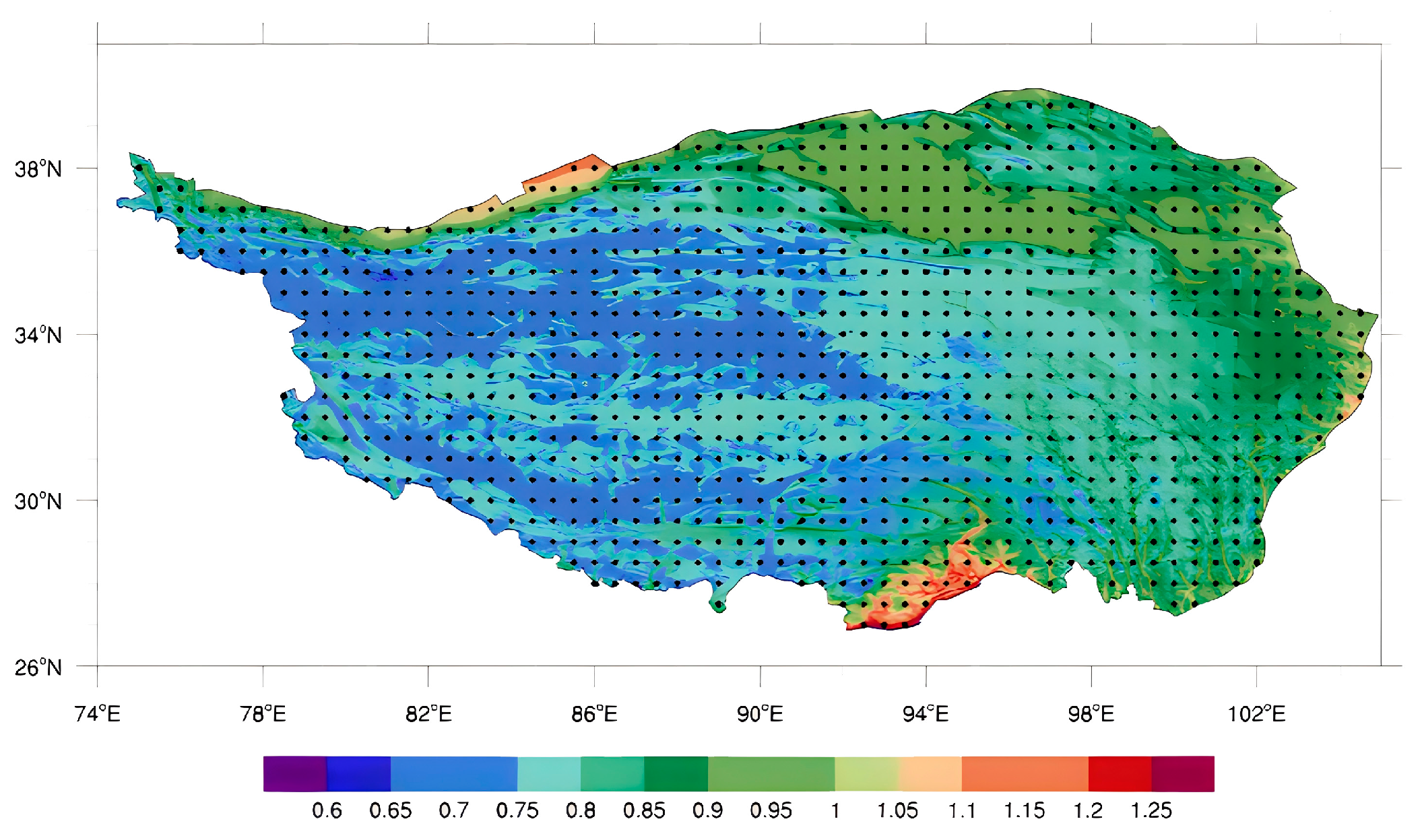
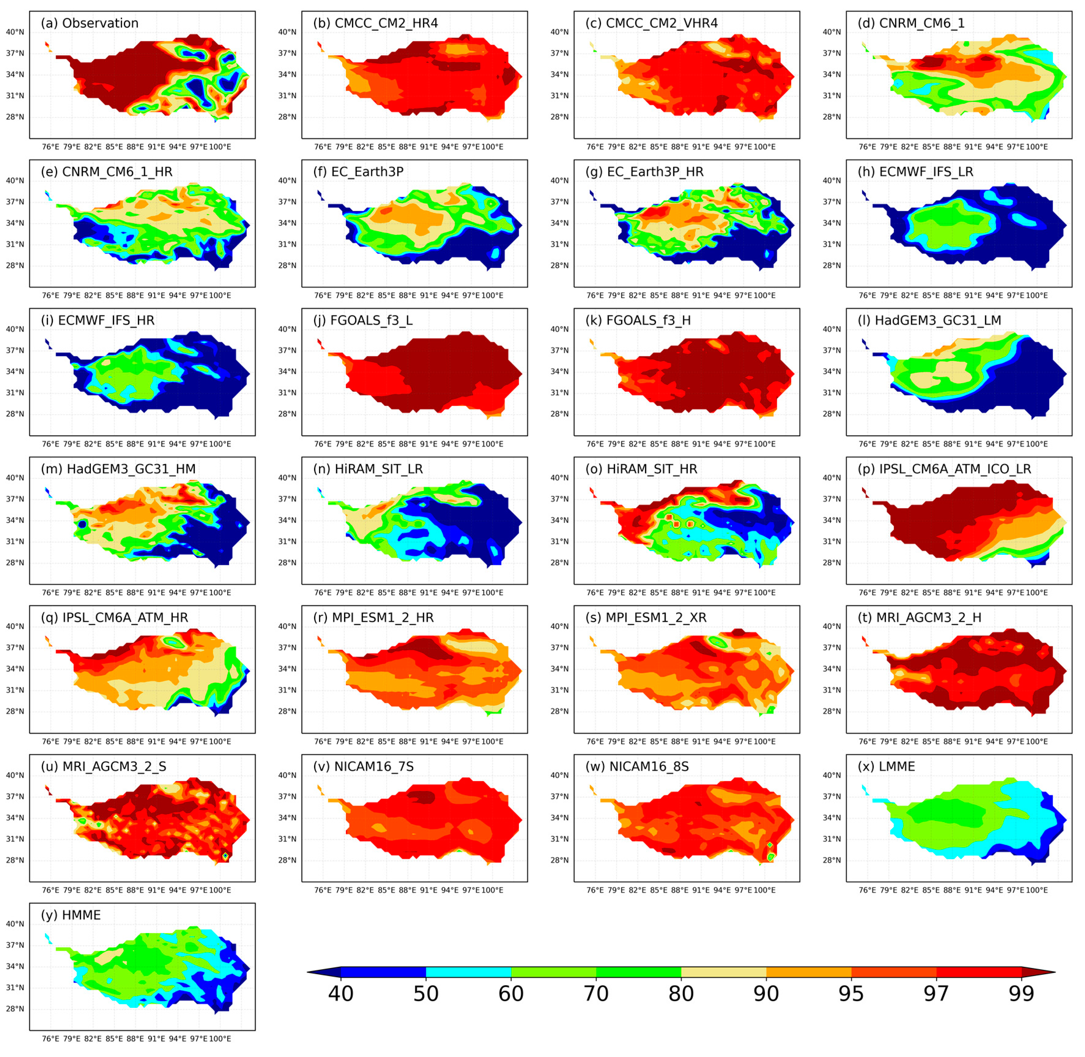
• In comparison with observations across the entire TP, CMIP6 models demonstrated a certain capability to simulate the climatological probability distribution of SWS. However, it is noteworthy that half of these GCMs, specifically CNRM-CERFACS, EC-Earth-Consortium, ECMWF, MOHC, and AS-RCEC, obviously underestimated the observed SWS. Conversely, the remaining GCMs tend to overestimate the SWS.
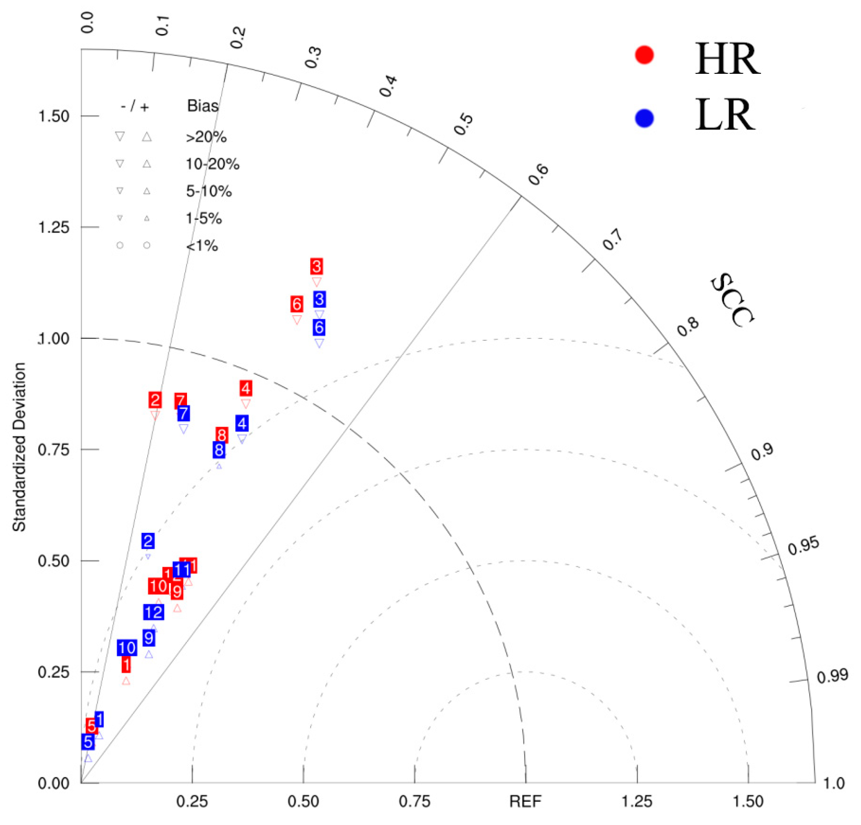
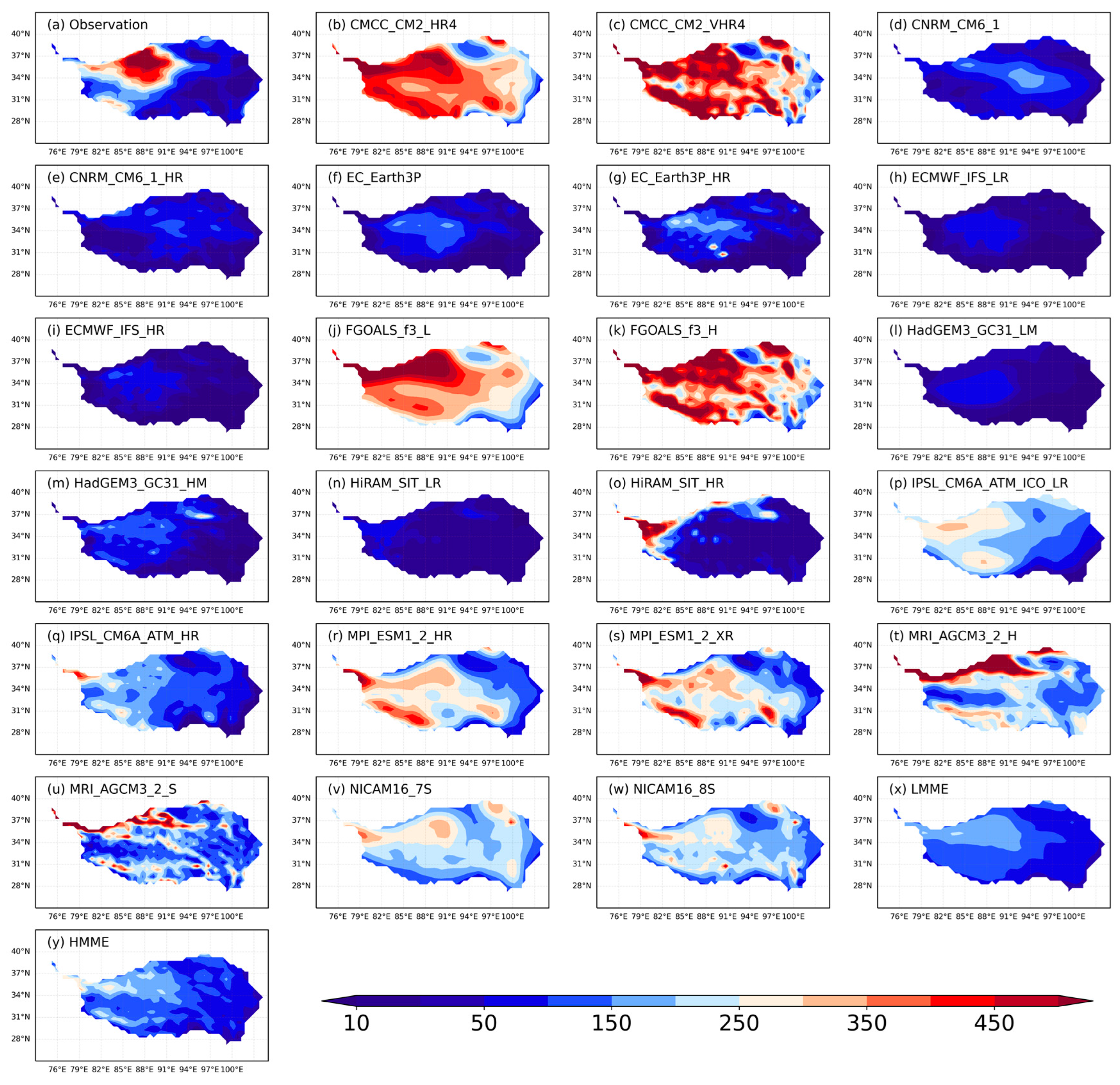
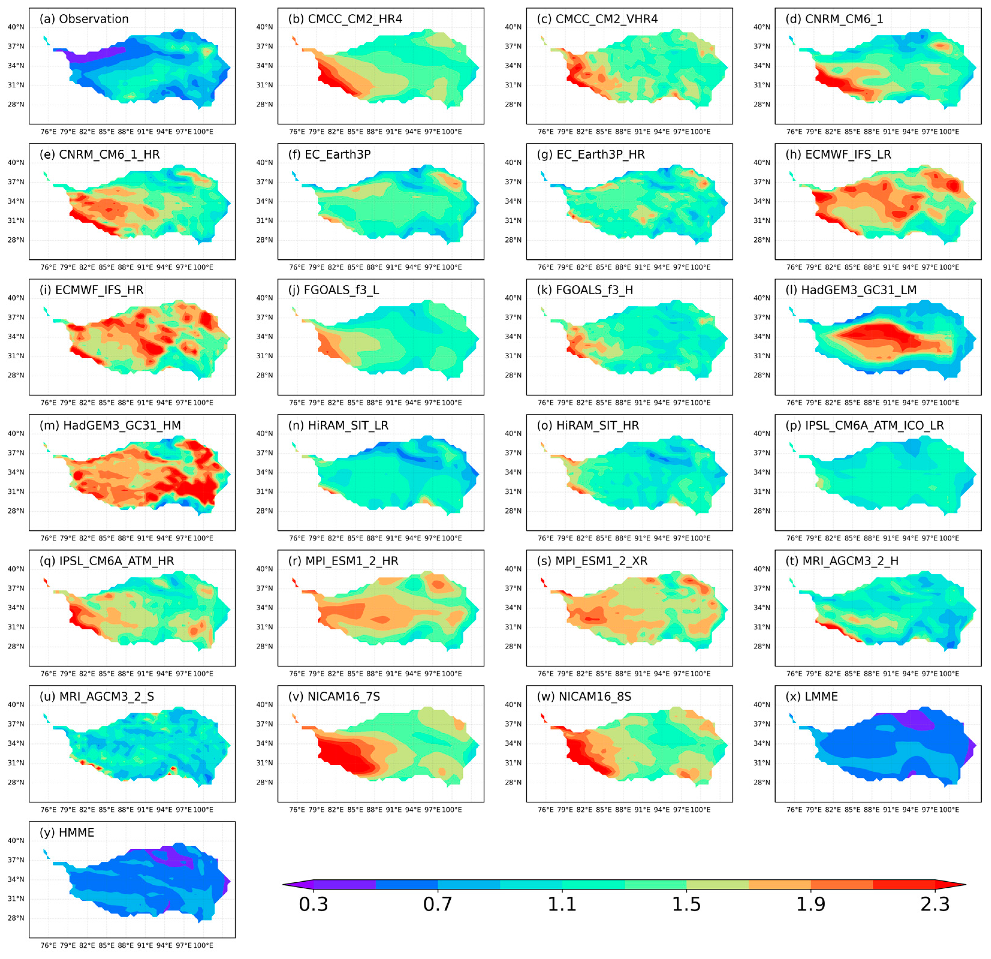
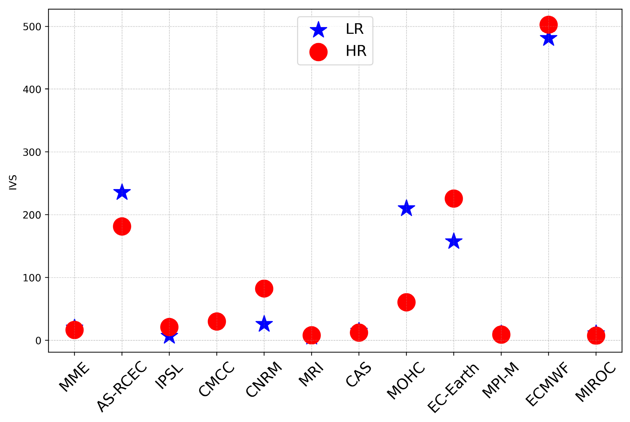
• Compared with the wind speed, the GCMs had larger biases in reproducing the other wind energy resources, such as WPD and EWH. In contrast, the biases in the MME were relatively smaller than most individual models and realistically simulated against observational data. Regarding the interannual variability, both the HR and LR models failed to capture the interannual variation in the WPD over the TP.
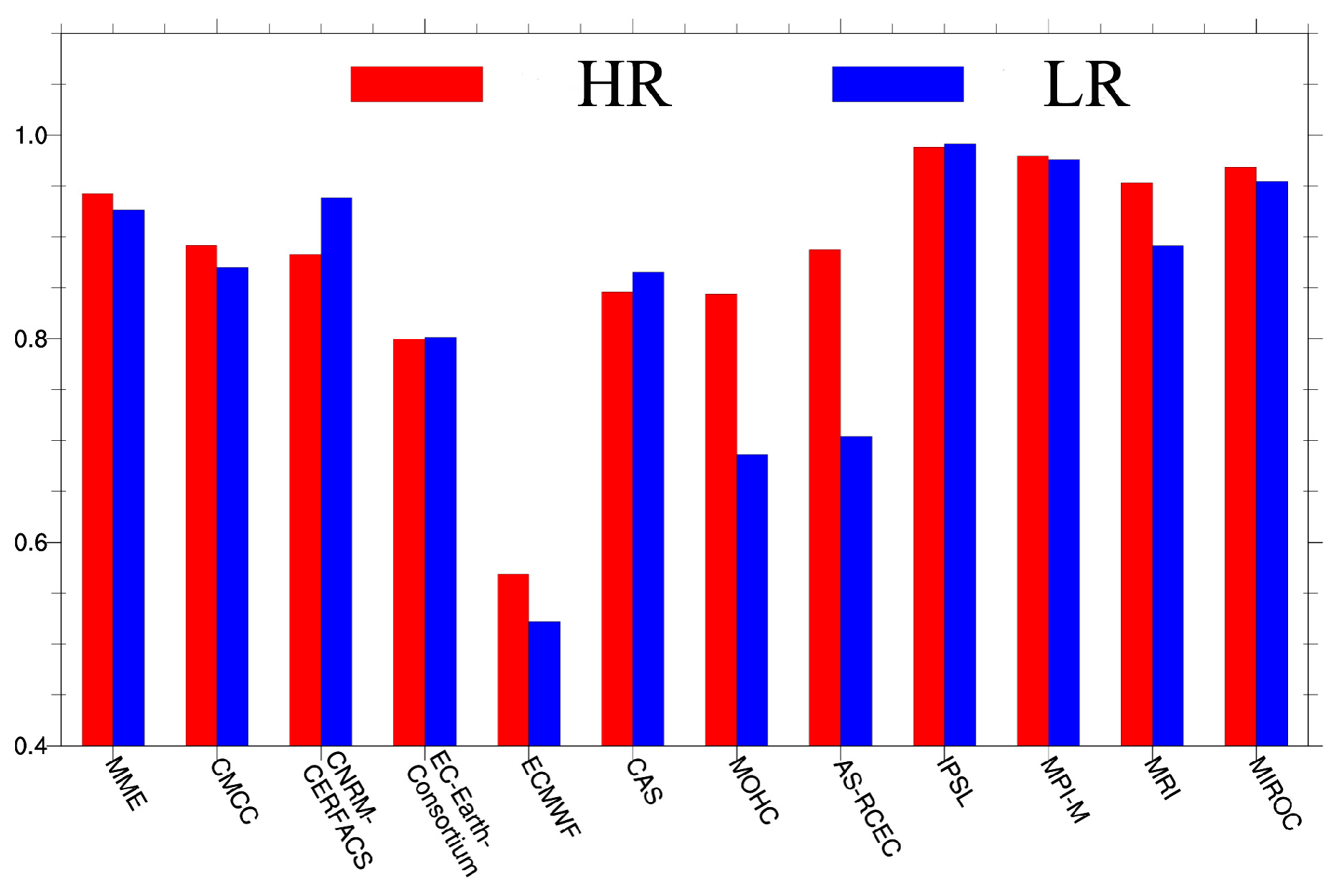
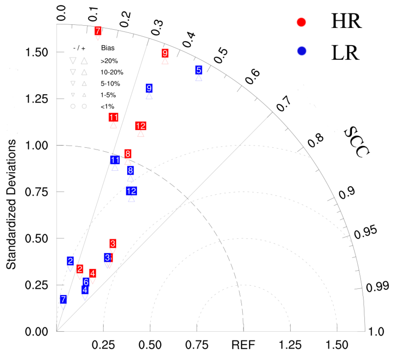
• More than half of the HR GCMs had a reduced bias relative to the corresponding LR GCMs. Most HR models exhibited good performance in simulating wind energy resources over the TP in terms of spatial patterns and temporal variability. However, the overall performance of the HR GCMs varied among models, which suggests that solely improving the horizontal resolution is not sufficient to solve the uncertainties and deficiencies in the simulation of wind energy completely over complex terrain.

The present paper provides a preliminary comparison of the performance of different horizontal resolution models in simulating wind energy over the TP. Although the horizontal resolution of current models has improved to some extent, large biases among the model simulations are still apparent not only in terms of the spatial pattern but also in terms of its temporal variability. Furthermore, the HR and LR versions of the same models both show considerably large uncertainties. The HR simulations of climate over the TP remain a formidable challenge for current GCMs because accurate representations of the dynamic framework and various physical processes associated with complex terrain are difficult to obtain. These limitations may be overcome to some extent through further model structure and physical improvement or downscaling of GCM outputs, ensemble simulations, and artificial intelligence techniques.

References

1. Hoogwijk, M.; de Vries, B.; Turkenburg, W.C. Assessment of the global and regional geographical, technical and economic potential of onshore wind energy. Energy Econ. 2004, 26, 889–919. [Google Scholar] [CrossRef]
2. Eurek, K.; Sullivan, P.; Gleason, M.; Hettinger, D.; Heimiller, D.; Lopez, A. An improved global wind resource estimate for integrated assessment models. Energy Econ. 2017, 64, 552–567. [Google Scholar] [CrossRef]
3. Wu, J.; Shi, Y.; Xu, Y. Evaluation and Projection of Surface Wind Speed Over China Based on CMIP6 GCMs. J. Geophys. Res. Atmos. 2020, 125, e2020JD033611. [Google Scholar] [CrossRef]
4. Da, Z.; Xiliang, Z.; Jiankun, H.; Qimin, C. Offshore wind energy development in China: Current status and future perspective. Renew. Sustain. Energy Rev. 2011, 15, 4673–4684. [Google Scholar] [CrossRef]
5. Wang, Q.; Qiu, H.-N. Situation and outlook of solar energy utilization in Tibet, China. Renew. Sustain. Energy Rev. 2009, 13, 2181–2186. [Google Scholar] [CrossRef]
6. Wu, J.; Xiao, J.; Hou, J.; Lyu, X. Development potential assessment for wind and photovoltaic power energy resources in the main desert-gobi-wilderness areas of China. Energies 2023, 16, 4559. [Google Scholar] [CrossRef]
7. Gao, Y.; Ma, S.; Wang, T.; Wang, T.; Gong, Y.; Peng, F.; Tsunekawa, A. Assessing the wind energy potential of China in considering its variability/intermittency. Energy Convers. Manag. 2020, 226, 113580. [Google Scholar] [CrossRef]
8. You, Q.; Fraedrich, K.; Min, J.; Kang, S.; Zhu, X.; Pepin, N.; Zhang, L. Observed surface wind speed in the Tibetan Plateau since 1980 and its physical causes. Int. J. Clim. 2013, 34, 1873–1882. [Google Scholar] [CrossRef]
9. Guo, X.; Wang, L.; Tian, L.; Li, X. Elevation-dependent reductions in wind speed over and around the Tibetan Plateau. Int. J. Clim. 2016, 37, 1117–1126. [Google Scholar] [CrossRef]
10. Zhu, X.; Wei, Z.; Dong, W.; Wen, X.; Zheng, Z.; Chen, G.; Liu, Y. Projected temperature and precipitation changes on the Tibetan Plateau: Results from dynamical downscaling and CCSM4. Theor. Appl. Climatol. 2019, 138, 861–875. [Google Scholar] [CrossRef]
11. Li, D.; Feng, J.; Dosio, A.; Qi, J.; Xu, Z.; Yin, B. Historical evaluation and future projections of 100-m wind energy potentials over CORDEX-East Asia. J. Geophys. Res. Atmos. 2020, 125, e2020JD032874. [Google Scholar] [CrossRef]
12. Deng, H.; Hua, W.; Fan, G. Evaluation and projection of near-surface wind speed over China based on CMIP6 models. Atmosphere 2021, 12, 1062. [Google Scholar] [CrossRef]
13. Zhang, S.; Li, X. Large scale wind power integration in China: Analysis from a policy perspective. Renew. Sustain. Energy Rev. 2012, 16, 1110–1115. [Google Scholar] [CrossRef]
14. Mohan, S.; Bhaskaran, P.K. Evaluation of CMIP5 climate model projections for surface wind speed over the Indian Ocean region. Clim. Dyn. 2019, 53, 5415–5435. [Google Scholar] [CrossRef]
15. Akinsanola, A.A.; Ogunjobi, K.O.; Abolude, A.T.; Salack, S. Projected changes in wind speed and wind energy potential over West Africa in CMIP6 models. Environ. Res. Lett. 2021, 16, 044033. [Google Scholar] [CrossRef]
16. Olaofe, Z.O. Review of energy systems deployment and development of offshore wind energy resource map at the coastal regions of Africa. Energy 2018, 161, 1096–1114. [Google Scholar] [CrossRef]
17. Carvalho, D.; Rocha, A.; Gómez-Gesteira, M.; Santos, C.S. Potential impacts of climate change on European wind energy resource under the CMIP5 future climate projections. Renew. Energy 2017, 101, 29–40. [Google Scholar] [CrossRef]
18. Mahajan, S.; Evans, K.J.; Branstetter, M.L.; Tang, Q. Model resolution sensitivity of the simulation of North Atlantic Oscillation teleconnections to precipitation extremes. J. Geophys. Res. Atmos. 2018, 123, 11392–11409. [Google Scholar] [CrossRef]
19. Kumar, D.; Mishra, V.; Ganguly, A.R. Evaluating wind extremes in CMIP5 climate models. Clim. Dyn. 2014, 45, 441–453. [Google Scholar] [CrossRef]
20. Reyers, M.; Moemken, J.; Pinto, J.G. Future changes of wind energy potentials over Europe in a large CMIP5 multi-model ensemble. Int. J. Clim. 2015, 36, 783–796. [Google Scholar] [CrossRef]
21. Costoya, X.; Rocha, A.; Carvalho, D. Using bias-correction to improve future projections of offshore wind energy resource: A case study on the Iberian Peninsula. Appl. Energy 2020, 262, 114562. [Google Scholar] [CrossRef]
22. Li, L.-L.; Li, J.; Yu, R.-C. Evaluation of CMIP6 HighResMIP models in simulating precipitation over Central Asia. Adv. Clim. Chang. Res. 2022, 13, 1–13. [Google Scholar]
23. Legates, D.R.; McCabe, G.J., Jr. Evaluating the use of “goodness-of-fit” measures in hydrologic and hydroclimatic model validation. Water Resour. Res. 1999, 35, 233–241. [Google Scholar] [CrossRef]
24. Jafari, S.; Sommer, T.; Chokani, N.; Abhari, R.S. Wind resource assessment using a mesoscale model: The effect of horizontal resolution. In Turbo Expo: Power for Land, Sea, and Air; American Society of Mechanical Engineers: New York, NY, USA, 2012; Volume 44724, pp. 987–995. [Google Scholar]
25. Tolentino, J.T.; Rejuso, M.V.; Inocencio, L.C.; Ang, M.R.C.; Bagtasa, G. Effect of horizontal and vertical resolution for wind resource assessment in Metro Manila, Philippines using Weather Research and Forecasting (WRF) model. In Earth Resources and Environmental Remote Sensing/GIS Applications VII; International Society for Optics and Photonics: Bellingham, WA, USA, 2016; Volume 10005, pp. 351–366. [Google Scholar]
26. Haarsma, R.J.; Roberts, M.J.; Vidale, P.L.; Senior, C.A.; Bellucci, A.; Bao, Q.; Chang, P.; Corti, S.; Fučkar, N.S.; Guemas, V.; et al. High resolution model intercomparison project (HighResMIP v1.0) for CMIP6. Geosci. Model Dev. 2016, 9, 4185–4208. [Google Scholar] [CrossRef]
27. Roberts, M.J.; Jackson, L.C.; Roberts, C.D.; Meccia, V.; Docquier, D.; Koenigk, T.; Ortega, P.; Moreno-Chamarro, E.; Bellucci, A.; Coward, A.; et al. Sensitivity of the Atlantic meridional overturning circulation to model resolution in CMIP6 HighResMIP simulations and implications for future changes. J. Adv. Model. Earth Syst. 2020, 12, e2019MS002014. [Google Scholar] [CrossRef]
28. Xin, X.; Wu, T.; Jie, W.; Zhang, J. Impact of higher resolution on precipitation over China in CMIP6 HighResMIP models. Atmosphere 2021, 12, 762. [Google Scholar] [CrossRef]
29. Zhang, W.; Villarini, G.; Scoccimarro, E.; Roberts, M.; Vidale, P.L.; Vanniere, B.; Caron, L.P.; Putrasahan, D.; Roberts, C.; Senan, R.; et al. Tropical cyclone precipitation in the HighResMIP atmosphere-only experiments of the PRIMAVERA Project. Clim. Dyn. 2021, 57, 253–273. [Google Scholar] [CrossRef]
30. Kim, H.-J.; Wang, B.; Ding, Q. The global monsoon variability simulated by CMIP3 coupled climate models. J. Clim. 2008, 21, 5271–5294. [Google Scholar] [CrossRef]
31. Demory, M.-E.; Berthou, S.; Fernández, J.; Sørland, S.L.; Brogli, R.; Roberts, M.J.; Beyerle, U.; Seddon, J.; Haarsma, R.; Schär, C.; et al. European daily precipitation according to EURO-CORDEX regional climate models (RCMs) and high-resolution global climate models (GCMs) from the High-Resolution Model Intercomparison Project (HighResMIP). Geosci. Model Dev. 2020, 13, 5485–5506. [Google Scholar] [CrossRef]
32. Wu, J.; Gao, X.J. A gridded daily observation dataset over China region and comparison with the other datasets. Chin. J. Geophys. 2013, 56, 1102–1111. [Google Scholar]
33. Zhou, Y.; Wu, W.X.; Liu, G.X. Assessment of onshore wind energy resource and wind-generated electricity potential in Jiangsu, China. Energy Procedia 2011, 5, 418–422. [Google Scholar] [CrossRef]
34. Wen, Y.; Kamranzad, B.; Lin, P. Assessment of long-term offshore wind energy potential in the south and southeast coasts of China based on a 55-year dataset. Energy 2021, 224, 120225. [Google Scholar] [CrossRef]
35. Taylor, K.E. Summarizing multiple aspects of model performance in a single diagram. J. Geophys. Res. Atmos. 2001, 106, 7183–7192. [Google Scholar] [CrossRef]
36. Cinner, J.E.; Caldwell, I.R.; Thiault, L.; Ben, J.; Blanchard, J.L.; Coll, M.; Diedrich, A.; Eddy, T.D.; Everett, J.D.; Folberth, C.; et al. Potential impacts of climate change on agriculture and fisheries production in 72 tropical coastal communities. Nat. Commun. 2022, 13, 3530. [Google Scholar] [CrossRef] [PubMed]
Figure 1. Spatial distribution of actual air density (kg·m−3) over TP. (The black dots represent the grid boxes with a resolution of 0.5° × 0.5°).
Atmosphere 15 01323 g001
Figure 2. Climatic means (1985–2014) of observed and simulated (both LR and HR) probability distributions (%) of region-averaged daily wind speed (m·s−1) at 100 m over the TP provided by 22 models from (bl) 11 institutes as well as their (a) MME. The cumulative distributions are presented in the upper right panel, with the black, red, and blue lines (bars) representing the observations and the HR and LR simulations, respectively.
Atmosphere 15 01323 g002
Figure 3. The IA of the probability distribution of the wind speed at 100 m over the TP simulated by the HR and LR models.
Atmosphere 15 01323 g003
Figure 4. (a) Observed and (by) simulated (both LR and HR) spatial distributions of EWH (%) at 100 m over the TP provided by 22 models from 11 institutes.
Atmosphere 15 01323 g004
Figure 5. Taylor diagram of HR- and LR- simulated EWH over the TP. The angular axes indicate the SCC between the simulations and observations, whereas the radial axes display the normalized spatial standard deviation (SSTD) relative to the observations. The dashed arc represents the CRMSE. The red and blue colors represent the HR and LR simulations, respectively. The numbers 1–11 represent different models (see Table 1), and the number 12 represents the MME. The symbols in the upper left panel denote the relative bias, and “REF” is the reference, representing the observed EWH.
Atmosphere 15 01323 g005
Figure 6. (a) Observed and (by) simulated (both LR and HR) spatial distributions of WPD (W·m−2) at 100 m over the TP provided by 22 models from 11 institutes.
Atmosphere 15 01323 g006
Figure 7. Taylor diagram of HR- and LR- simulated WPD over the TP. The angular axes indicate the SCC between the simulations and observations, whereas the radial axes display the normalized SSTD relative to the observations. The dashed arc represents the CRMSE. The red and blue colors represent the HR and LR simulations, respectively. The numbers 1–11 represent different models (see Table 1), and the number 12 represents the MME. The symbols in the upper left panel denote the relative bias, and “REF” is the reference, representing the observed WPD.
Atmosphere 15 01323 g007
Figure 8. (a) Observed and (by) simulated (both LR and HR) spatial distributions of CV at 100 m over the TP provided by 22 models from 11 institutes.
Atmosphere 15 01323 g008
Figure 9. IVS of HR and LR simulations for WPD over the TP.
Atmosphere 15 01323 g009