Review

The Significance of Internal Variability for Numerical Experimentation and Analysis

1
Meteorological Institute, Hamburg University, 20148 Hamburg, Germany
2
Max-Planck Institute of Meteorology, 20146 Hamburg, Germany
*
Author to whom correspondence should be addressed.
Atmosphere 2024, 15(11), 1317; https://doi.org/10.3390/atmos15111317
Submission received: 25 July 2024 / Revised: 24 October 2024 / Accepted: 24 October 2024 / Published: 1 November 2024
(This article belongs to the Section Atmospheric Techniques, Instruments, and Modeling)

Abstract

:
When regional (limited-area) models of the hydrodynamics of the atmosphere and ocean are run over an extended time, variability unrelated to external “drivers” emerges: this variability is colloquially named “hydrodynamical noise” or just “noise”. This article summarises what we have learned in the past few years about the properties of such noise and its implications for numerical experimentation and analysis. The presence of this noise can be identified easily in ensembles of numerical simulations, and it turns out that the intensity of the noise is closely linked to scale-dependent “memory”. The “memory” in the atmosphere and ocean describes the persistence of atmospheric and oceanic conditions, usually quantified by an autocorrelation function. At the system level, this “memory” term, as given by Hasselmann’s stochastic climate model, plays a key role. In the case of marginal seas, the process of baroclinic instability modulated by tides and the formation of seasonal thermoclines are significant aspects. Some more general aspects are discussed, such as the applicability of the stochastic climate model to systems outside of atmospheric and oceanic dynamics, for example, biogeochemical systems, the irreversibility of tipping points, the challenges of detecting changes beyond a noise level, and the attribution of causes of change.

1. Introduction

Atmospheric and oceanic variability arises from the external forcing (for example, solar radiation) and internal processes associated with the nonlinearity and multi-scale integrations within a system [1]. Such variability caused by internal processes is called internal variability, which is intrinsic, unprovoked, and cannot be linked directly to external forcing or the details of the initial state [2]. Studying internal, unprovoked variability in observational data of the atmospheric and oceanic processes is difficult; there are baroclinic disturbances in the atmosphere, which are a manifestation of such variability, but that their ability to form spontaneously only became clear when atmospheric models became available in 1970 for extended simulations, allowing the analysis of unprovoked variability. The challenge of how to determine the “noise level” and how to perform statistical tests was introduced by [3,4]. Thus, the recognition of internal variability dates back approximately 50 years. Please note in this study, “noise” refers to deviations from the average state due to internal variations.
A nice illustration of the formation of such unprovoked variability is provided by Fischer’s experiment [5], which ran an aqua-planet experiment initiated at a state of rest, i.e., with zero wind. Figure 1 shows the development of general circulation from a state of rest. The smooth part of the development is mostly externally enforced (the latitudinally different heat uptake of the Earth’s surface), but the details are not and would not be repeatable if another identical simulation were carried out. Initially, the state is remotely different from any truly occurring natural state. During the first, say, 10 days, the atmosphere remains in a state of rest, but then general circulation begins to emerge, in particular baroclinic storms at Northern and Southern Hemisphere mid-latitudes. The time-lapse of the appearance of general circulation is for the inertia of the system (and the model). After the first 20–30 days, variations around the mean characteristics remain, and these variations are “noise”, i.e., the internal variation of the atmosphere.
Such a recognition of the presence of noise generated in regional models of the atmospheric dynamics took much longer because of a tacit understanding that any such possible variability would quickly be wiped out by continuously updated lateral boundary conditions. However, when ensembles of simulations in the regional model were eventually integrated [6,7], it quickly became clear that relevant intra-ensemble variability would form [8]. The tendency to build internal variability depends on the size of the integration area: in small areas, the noise level becomes very small (e.g., [9]); in large areas, substantial noise forms, see, e.g., [10].
In the ocean, the recognition of internal variability had to wait much longer until the availability of satellites, which showed the ubiquity of mesoscale eddies and other mesoscale features (Figure 2). Since the early 2000s, studies evaluating ensembles of ocean simulations began to be published, and with them, the recognition of internal variability formed in the ocean, and not just of that inherited from the atmosphere. Leading examples included Jochum and Murtugudde [11,12], Arbic [13], and Sèrazin [14]. The first systematic analysis of the formation and characteristics of internally generated variability in the global ocean was conducted by Penduff et al. [15].
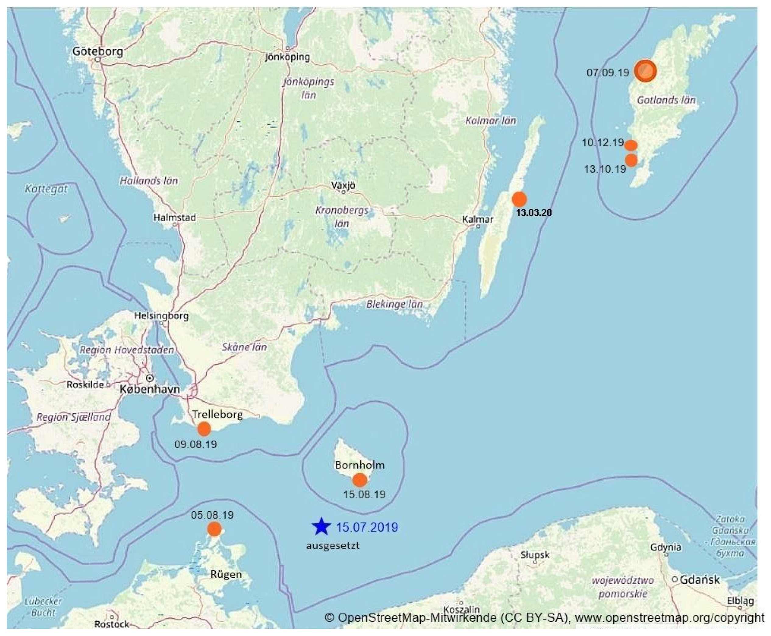
The question of internal variability in marginal seas was taken up even later, even if the observation of divergent trajectories of tracers was long understood (Figure 3). The pioneers were Büchmann and Söderkvist [17], Waldman et al. [18], Tang et al. [19,20], Lin et al. [21,22], and Benincasa et al. [23], who implemented the ensemble framework (see Section 3). Tang demonstrated for the South China Sea that increasing the horizontal spatial resolution leads to the formation of more intrinsic variability and that external forcing is dominant for large scales, while that of small scales is mostly internally generated. Lin et al. [22], on the other hand, found the tendency to generate internal variability to be dependent on the presence of tides and a seasonal thermocline. They demonstrated the significance of baroclinic instability in forming noise [24], consistent with the results of Waldman et al. [25]. More information on this will be provided in Section 3.1.
The concept that climate is not static but rather undergoes variations across all time scales has been recognised for a considerable period, as evidenced by works such as those of Brūckner [27] in 1890 and Mitchell [28] in 1976 (cf. Figure 4). Figure 4 (right panel) is a sketch by J. Murray Mitchell from 1976; it shows a series of peaks pointing towards external influences, but between these peaks, the variance is not zero but displays a continuous and smooth spectrum, which can hardly be due to an external cause, if that is not itself continuous and smooth. However, such forcing is not known. The figure is not based on data but a mental construction of the cited author; therefore, it could be different for different variables, such as temperature or thermal energy. The debate surrounding whether these variations stem from anthropogenic sources, particularly deforestation, or are intrinsic to Earth’s internal processes (referred to as “cosmic” processes) has been ongoing since at least the mid-19th century, if not earlier, extending beyond academic circles to encompass political discourse.
In 1976, Klaus Hasselmann [1] introduced an alternative mechanism, proposing the integration of short-term, small-scale weather fluctuations (such as atmospheric storms and oceanic eddies) in systems with significant “memory”. A detailed explanation of the stochastic climate model can be found in Section 2. This proposition, articulated in his “Stochastic Climate model,” among other achievements, ultimately earned him the Nobel Prize in Physics in 2021.
The challenge to “detect” and characterize such “unprovoked variability” and to “attribute” plausible causes and processes to their emergence has persisted to some extent. In global atmospheric dynamics, detection became straightforward once global general circulation models of the atmosphere could be integrated over extended periods or in ensembles of simulations. Similarly, attribution was relatively uncomplicated, given the recognition of baroclinic instability since the time of Vilhelm Bjerknes [29].
In contrast, the detection and attribution process for the global ocean occurred much later, coinciding with the availability of eddy-permitting models and high-resolution satellite imagery of the ocean surface. Similar delays were observed in the case of regional atmospheric and oceanic systems, where detection efforts were initially limited. However, pioneers in ocean noise research like Penduff [15] shed light on macro-scale internal variability. Waldman [18] and Lin [24] determined the dominant role of baroclinicity in amplifying small-scale variations to large-scale variability. Nonetheless, other processes may also contribute to the formation of macro-scale noise.
The emergence of macro-scale noise carries three significant implications. The motivation of this article is to illustrate the following challenges:
  • Firstly, noise is expected to arise in systems influenced by short-term weather variations, which lack strong damping but possess robust memory. Such systems are foremost all atmospheric and oceanic hydrodynamical systems with short-term variations related to eddies, internal tides, fronts, and other phenomena. A very different case of such systems encompasses regional morphodynamics, as highlighted by a CNN report (see “Damaged US Navy sub was operating in one of the world’s most difficult undersea environments, analysts say”, CNN, 8 October 2021) following a US submarine incident in the South China Sea, which emphasised the ongoing, albeit gradual, changes in the environment and seafloor. This underscores the necessity for continuous bottom contour mapping in the region. Additionally, ecosystem dynamics may also be affected by such noise [30,31,32].
  • Another aspect pertains to the realm of numerical experimentation, where alterations in factors such as parametrisations, boundary conditions, and atmospheric composition are introduced in simulations. In such experiments, appropriately designed ensembles are crucial for estimating the extent of inherent variability, determining whether changes between ensembles can be attributed solely to internal variability or if external factors play a role (an issue akin to detection) (e.g., [33]).
  • The third one is the conventional “detection and attribution” challenge [34]: whether observed variations may be understood in the framework of internal variability or if an external factor needs to be determined to explain the observed change, which brings us back to the initial observations of the need to separate forced and unforced climate variations, which was mentioned at the beginning of this paper.

2. Methods

The “Stochastic Climate Model” was originally introduced by Klaus Hasselmann [1] in 1976, and its applicability was demonstrated by [35,36,37]. Originally, it was quite a challenge to understand the concept, but as people got more used to it, it became really simple. When considering stationary solutions of the dynamics x of a not-too-nonlinear process y,
d y d t = F ( y ) ,
with dynamics F ( y ) ; the dynamics of the slow components x may often be approximated by a linear stochastic system:
d x d t = α × x + ϵ ,
or
x t + 1 = α × x t + ϵ t + 1 .
This formulation is based on the assumption that the slow part of y, named x, is exposed to the action of the fast components of y labelled ϵ . Thus, the slow component x of y is driven by a “memory-term” α and a stochastic “forcing” component ϵ t + 1 , representing the fluctuations of the fast component of y. In many cases, it is assumed that ϵ is a white noise “no memory”-process. A solution is obtained by integrating Equation (1) over time, which contains an integration of ϵ over time. To obtain a stationarily varying solution from Equation (1), it must incorporate negative feedback, namely the memory term.
The stochastic climate model is an idealised theory model, which is subject to short-term fast variability and will show long-term, slow variation as an integrated response. In the spectral representation, white noise is integrated into a red spectrum, with enhanced variance at longer scales because of the existence of stochastic “forcing”. The value of α determines the memory of the system, with a larger α indicating an extended memory and a redder spectrum; a smaller α indicates shorter memory and a less-red spectrum.
More complex approximations than (2) are, of course, possible, but (3), named “Ornstein–Uhlenbeck” or “autoregressive process of 1st order” (AR-1), have turned out quite successful [38].
The key parameter in (3) is the memory term α , which controls the time within which a random excursion, excited by ϵ , is decaying. A useful approximation is the lag-1 auto-correlation of x. A larger α accompanies slower decay of the auto-correlation function with more variance at slow frequencies of the auto-spectrum [38]. For two values of α , namely 0.3 and 0.9, the auto-correlation function as well as the auto-spectra are displayed in Figure 5.
The main messages of the stochastic climate model are as follows: first, short-term variability matters for overall variability, which turns out to be a mixture of more or less sharp spectral peaks related to specific periodic forcing, such as daily or annual cycles, and the smooth spectrum of random forced variations (as depicted in Mitchell’s sketch, cf. Figure 4 (right panel)); second, given the same noise-seeding, a system with a larger memory generates higher long-term variability.

3. Results

The work on unprovoked variability in marginal seas is based on work by Chinese students, supervised by Hans von Storch [39] at the Helmholtz-Zentrum HZG in Geesthacht.

3.1. Emerging Noise in Marginal Seas

The study of emerging noise in marginal seas began with the analysis of hydrodynamic variability in the South China Sea. First, Meng Zhang [40] was tasked with conditioning ocean eddy statistics to the large-scale state of the South China Sea. Analyzing a multi-decadal simulation of an eddy-permitting ocean model of the South China Sea, good statistics of these eddies could be derived, but efforts to condition their statistics failed: the eddy activity mostly turned out to be a manifestation of internal processes.
Based on this result, Shengquan Tang [19,20] focused on internal variability in an extended simulation of the hydrodynamics of the South China Sea, its dependency on scales, and the model grid resolution. To do this, he used a hydrodynamical model of the near global ocean south of 54° N and north of 30° S with a grid resolution of 1°, an embedded West Pacific model with a grid resolution of 0.2°, and an embedded model of the South China Sea with a grid resolution of 0.04° (see Figure 1 in [19]). For forcing, atmospheric fluxes of momentum and heat were calculated for each calendar month and averaged across many years. In this way, climatological forcing was constructed (the climatological forcing only considers monthly variation) without weather variation but with an annual cycle.
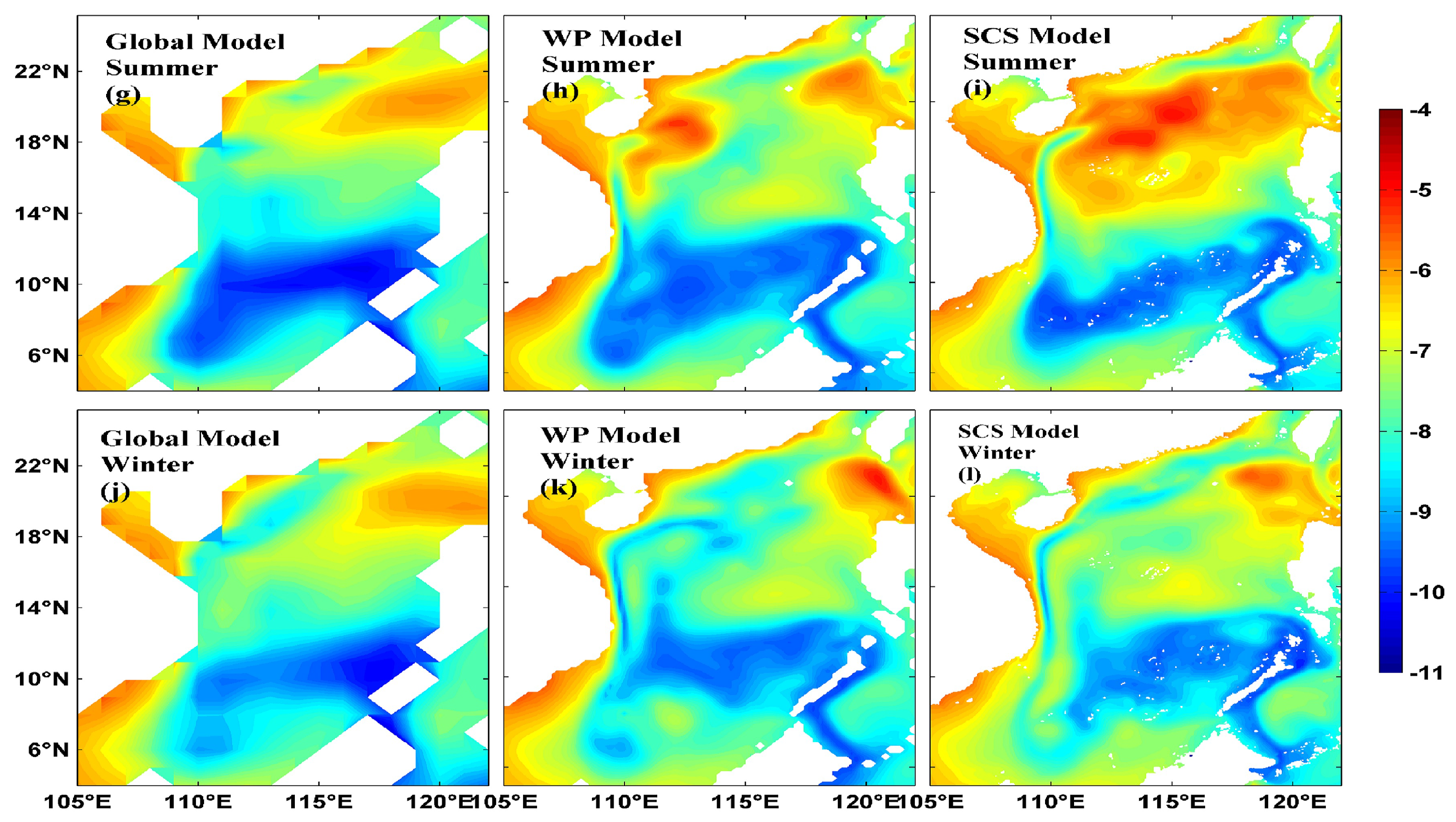
Figure 6 demonstrates, first, that there is variability in times scales (of days) when the regional ocean numerical model is forced by climatological forcing without corresponding daily variation. Thus, daily variability is internally generated. Second, the “noise” level, i.e., the intensity of unprovoked variability increases with enhanced grid resolution, and third, at least for the high-resolution model, noise is larger in summer than in winter, which has been hypothesised as being an effect of the presence of stronger seasonal thermocline [23,41].
The next step in Tang et al.’s analysis [20] was to decompose the simulated fields in components of different scales (spatial and temporal scales; usually, large spatial scales correspond to small temporal scales, and vice versa). To do so, an EOF analysis of simulated fields was conducted. The purpose of an EOF analysis is to derive a measurement of scale for different EOFs.
The auto-correlation of EOF patterns (in space) describes the correlation between different model grid points (similar to the autocorrelation in time, which represents the correlation between different time lags, but for auto-correlation in space, it concerns space lags). The spatial scale of that EOF is then the length when the auto-correlation calculated jointly across all grid points falls below a certain threshold. It turned out that the lower the EOF index, i.e., the more variance it would represent, the larger the spatial scales (Figure 5 in [20]).
Tang et al. [20] ran ensembles of four simulations for the year 2018. The members of the ensembles were identical apart of the model starting time and the length of the integration time, which covered the full year of 2008 (see Section 3). The EOF results show that there are three ranges of EOF indices, namely, EOFs 1–10, EOFs 11–50, and 50–1463. Within the three ranges, the signal-to-noise ratio has characteristic distributions. The first block of EOFs (1–10) has a large scale, namely with a spatial scale of 220 km on average, the middle block of EOFs (11–50) is “mid-scale”, with a middle scale of on-average scale of 110 km, and the remaining EOFs, with scales of about 30 km, are considered small-scale.
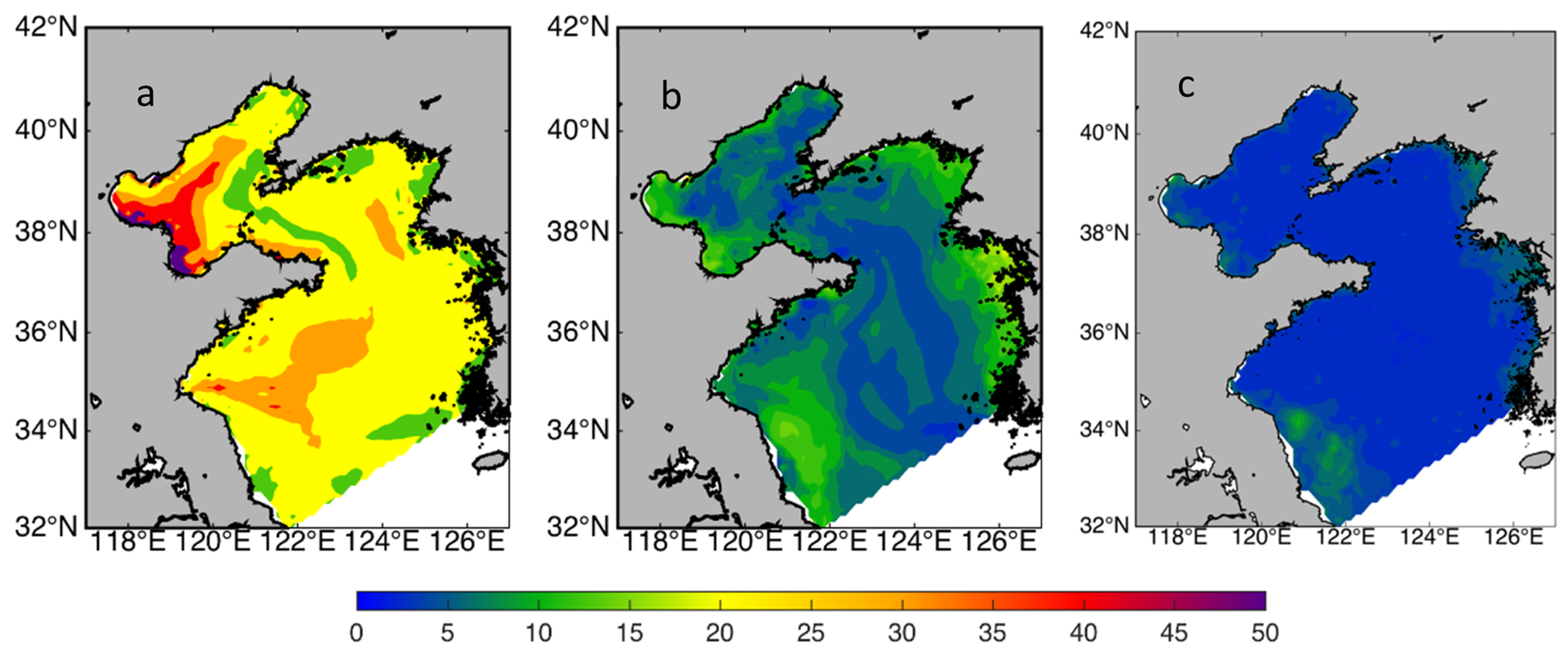
For each of the EOFs, daily time series’ of principal components are available for the four ensemble members: the daily means across the ensemble are considered deterministic, while the deviations on each day are noise. The “noise level” is determined as the 2008 time mean of the daily noise, and the “signal” is the standard deviation of the daily mean across the ensemble. The signal-to-noise level became smaller and smaller for growing EOF numbers: internal variability dominated for small scales, while the signal was only large for large scales (see Figure 8 in [20]). Figure 7 shows this for the case of the Bo Hai and Yellow Sea.
The South China Sea is mostly a deep marginal sea. Lin et al. [21] began their work by demonstrating that the results of Tang et al. [19,20] would also apply to the rather shallow Bo Hai and Yellow Sea. They hypothesised that the emergence of internal variability would be strongly damped if the tides were active; thus, they built ensembles with tides turned on and turned off. Indeed, the noise level was strongly decreased for large- and mid-scale disturbances when the tides were active, while the signal was found to be mostly unchanged.
In this first paper by Lin et al. [21], the hypothesis was voiced that this sensitivity to noise generation may be explained in the framework of the stochastic climate model (Section 2).
The issue of detecting the emergence of hydrodynamical noise was taken up by Benincasa et al. [23] for the case of the Mediterranean Sea. The numerical experiment was, in principle, the same, but it was a different model. The ensemble was much larger. A potentially more significant difference was that the previous model’s simulations were forced with given fluxes, while Benincasa used fluxes as derived through bulk-formula parametrisations. “Intrinsic variability displayed a distinct seasonal cycle in the surface layers, with a prominent maximum at around 30 m depth during the summer probably connected to the summer thermocline formation processes” [23].

3.2. Sensitivity to Tides and Changing Seasonal Conditions

Lin’s other paper [22] focused on the applicability of the stochastic climate model to understanding the seasonality of the formation of noise and the sensitivity to the presence of tides. To do so, she derived the memory α (see Section 2) and compared this with the slopes of the auto spectra of noise-variability for each principal component time series.
This study yielded two primary outcomes. Firstly, indications were found of an underlying low-dimensional dynamical core with relatively sluggish fluctuations, which facilitates the transfer of short-term internal variability to longer timescales in the Bo Hai and Yellow Sea. This aligns with Hasselmann’s concepts of both the stochastic climate model (SCM) and PIPs-and-POPs (principal interaction patterns and principal oscillation patterns) [42]. The POPs concept may be seen as a generalisation of the SCM but also as a simplification of the rather general concept of principal interaction patterns (PIPs), which asks for the determination of a few patterns whose coefficients allow an optimal prediction of the slow variations of the considered system. Second, as predicted by the SCM, a modification of the memory is associated with a corresponding adjustment in the long-term variance, particularly on a large-scale basis.
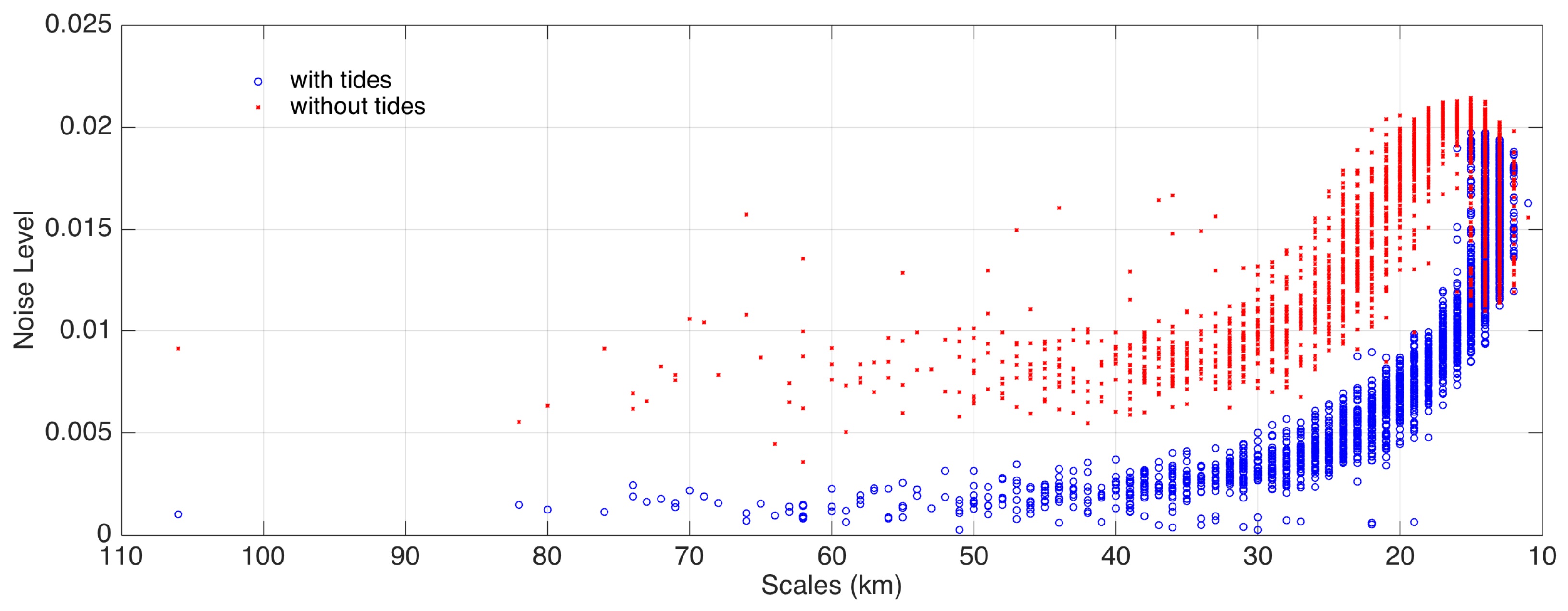
Active tides limit the generation of large-scale internal variability (Figure 8; large scales are associated with long-term variability.) Also, memory is strongly reduced when tides are active (Figure 9), or in other words, tides block the accumulation of unprovoked variability on spatial scales of 30 and more kms and reduce characteristic times (memory). The auto-spectra of leading principal components also become considerably flatter and their slopes get smaller, all of which is predicted by the stochastic climate model (3). The understanding is that tides dissipate random disturbances so that they cannot develop for a longer time and build persistent large-scale anomalies.
When comparing the situation in winter to that in summer, similar results are found. In winter, when there is hardly a thermocline, the generation of internal variability is weak, but in summer, when a clear thermocline is present, much less so (see Lin et al. [22], but also Figure 10).
This is an analysis on the system level, but the question remains, which processes are responsible? Using the hypothesis of modified baroclinicity, Lin et al. [24] calculated the intensity of internal variability and the Eady estimate of theoretical diffusivity for pairs of ensembles “with/without tides” and ensembles for “winter/summer”. They found expected changes (namely internal variability increase with baroclinic instability increase), consistent with Waldman’s [18] and Benincasa’s [23] results.

3.3. Seeding Noise

Ensembles of extended simulations using regional atmospheric and oceanic models were initially conducted by varying the initialisation time. This allowed the models to have different spin-up periods of different lengths before the period of interest. During the spin-up period, which lasted a few months, the same oceanic forcing (sea surface temperature and lateral atmospheric forcing) or atmospheric forcing (vertical fluxes at the surface and lateral oceanic forcing) was applied. Consequently, the entire simulation period, including both the spin-up and experimental phases, remained consistent and identical across the different ensemble members during overlapping times [8,20].
By coincidence, identical simulations using the same limited area model code, initial conditions, and forcing conditions but performed on different computer platforms became available, first in atmospheric sciences and later in oceanography. The intensity and timing of deviations across different ensemble members were statistically identical [41,43]. In Geyer’s study, the exact same numerical simulation was run on different supercomputer platforms, namely, two platforms at Deutsches Klimarechenzentrum (DKRZ) and one platform at the Swiss National Supercomputing Centre (CSCS), Leibniz-Rechenzentrum (LRZ), Zentralanstalt für Meteorologie und Geodynamik (ZAMG), and Deutscher Wetterdienst (DWD). In atmospheric models, the periods of divergence were shorter and appeared to be influenced by the strength of the flow at the lateral boundaries, whereas in ocean models, it was very likely affected by the seasonal strength of the thermocline.
For each day, when all members of both ensembles, those generated using different times of initialisation and by using different computing platforms, were available, daily mean values across each ensemble, as well as the standard deviations of the deviations from these means, were calculated. Figure 10 shows these time series for the atmospheric case of a Northern European regional model (top) and the oceanic case of a regional model of the Bo Hai and Yellow Sea (bottom).
Minuscule changes, whether in the initial state or caused by different compilers, can trigger significant and persistent deviations. The way these small changes are introduced is irrelevant. This phenomenon, where unavoidable small disturbances grow to substantial spatial scales and intensities, aligns with the stochastic climate model theory. Such sensitivity to minor disturbances is not necessarily indicative of chaotic processes and can even occur in linear systems. A memory term α , which may vary over time, is required. These variations can be due to factors like the strength of the constraining boundary values [43] or seasonal variations in baroclinic stability [24].

4. Discussion

In the “motivation” Section 1, some implications of the presence of hydrodynamic noise have already been touched upon. Here, we deepen this discussion further.

4.1. First Experiments of the Effect of Disturbances on Morphodynamics

A main conclusion in Section 3 was that the stochastic climate model concept (Section 2) applies not only to the classical oceanographic and atmospheric cases documented in the literature but also to the hydrodynamics of marginal seas: whenever a system is not too nonlinear with limited damping, significant internal variably should emerge. Thus, observation led to the hypothesis that such variability should occur in other areas as well, such as in morphodynamics.
To do so, a simple model of the morphodynamics of a small bay with a narrow entry to the open sea was considered [44]. The ocean influenced the bay through a mono-frequency tide. Initially, the morphology was uniform, but over time, a variety of channels formed. Without any noise seeding, the distribution of the channels was symmetric, as no Coriolis force was active in this setup.
Hydrodynamical noise is excited by adding small disturbances to tidal variation for the first 20 tidal cycles, i.e., during the first 10 days. The Figure 11 shows how these small initial disturbances diverge within 240 years. While the general pattern is the same, with mostly two major channels through the entry of the bay, the details are all different. Small initial disturbances lead to an ensemble with significant variations of all channels, not only the large ones.
Thus, we developed the hypothesis that the development of morphodynamics depends on the inertial disturbance, but a closer inspection leads to the conclusion that once the system follows a certain trajectory, this continues without variation. Thus, long-term variations do not emerge. This system behaves like Figure 12a and not like Figure 12b. The system seems to have many stable points, given by different channel configurations, but hardly any low-frequency variations. Thus, this case is not to be explained by the SCM but by an extreme sensitivity to the initial state. That no low-frequency variability emerges, exemplified by a change in the channel system, may be due to too-strong damping; future numerical experiments with ongoing noise-seeding will be carried out to determine if such variations among different channel systems will emerge.

4.2. Assessing the Outcome of Numerical Experiments

An aspect of assessing the outcome relates to numerical experimentation, where changes in factors such as parameterisations, boundary conditions, and atmospheric composition are introduced into simulations [3]. In these experiments, appropriately designed ensembles are crucial for estimating the extent of inherent variability. This helps to determine whether changes between ensembles can be attributed solely to internal variability or if external factors play a role.
If “something” is expected to produce a certain effect, whether in the real world represented by observational data or in numerical simulations, it is simplistic to assume that the difference between the state when the “something” is active and the state when it is not active would accurately represent this effect or the “signal”.
Recognising the presence of variations unprovoked by the “something” using the technique of statistical hypothesis testing with the null hypothesis H0: <“something” has no effect> is appropriate. If this null hypothesis is rejected with a sufficiently small risk, then a valid conclusion is that an external factor is active. In the case of a numerical experiment with an active and a passive “something,” the external factor is indeed the “something”. However, in the case of observational data, there may be a variety of factors changing the observational record.
The determination of whether a “something” is active is called “detection”; the presence of a “signal is detected”, but it is not necessarily clear which factor is causing this signal. If a variety of candidates for the change exists, then the process of determining the most plausible mix of factors is determined: a process called “attribution”.
The term “(statistical) significance” in science refers to a statistical assessment of the probability that a given event is drawn from a given population representing the null hypothesis (even if ”significance” is also used in ordinary English, as in this article). If this probability is small, then the null hypothesis that the “event is consistent with standard conditions” is rejected, and the alternative, i.e., the “event is evidence for the presence of non-standard conditions”, is accepted. If it is “not small”, then the null hypothesis is “not rejected”, and the alternative hypothesis is also not accepted. The choice of “small” is subjective; in our field, it is usually 5%.
“Local” tests need to be carried out at grid points but could be conducted in any other representation of the fields, say EOFs, and then only with components of interest, such as at large scales. Hasselmann [34,46] suggested different strategies (see [47]).
A problem arises when such a test is carried out at many grid points. This is well-known among global atmospheric modellers, but possibly less so among regional modellers. If the null hypothesis is valid at all of these grid points, then one would expect, on average, the null hypothesis to be falsely rejected at 5% of them. The number of false rejections is in and of itself a random variable, and the percentage of rejections may be much larger, 20% or so. If, however, the rate is larger than, say, 20%, it is unlikely that all rejections are false, but some are valid. For further details on this aspect, refer to the textbook [38].
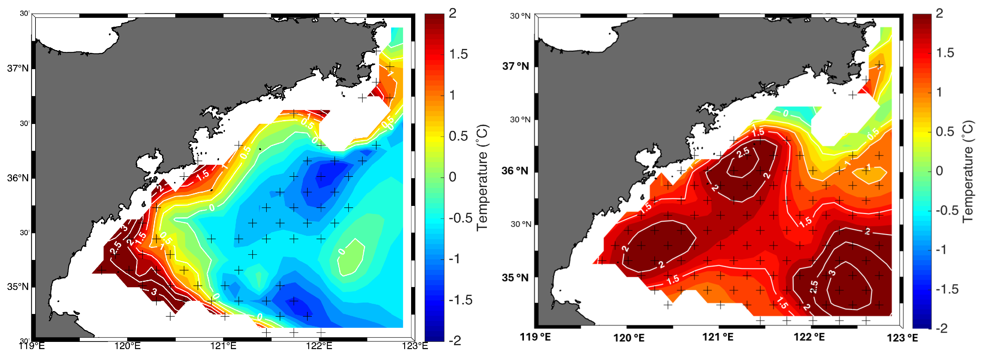
An example of such testing is that of a numerical experiment on the formation of a seasonal cold water pool off Qingdao in Figure 13 [33]. Here, the effect of tides as well as of variable winds is examined; three ensembles were built with both tides and realistic wind variability, one without tides and one with zero wind. Points where the null hypothesis is rejected are marked with crosses, which are 51% and 90% of all grid points, indicating global significance (i.e., not the effect of doing multiple local tests). The null hypothesis that tides and wind forcing have no effect is untenable.
For regional oceanographers, it seems that it is uncommon to examine their numerical sensitivity experiments.

4.3. Detection and Attribution

Another challenge is the “detection and attribution” problem in climate change studies, which involves determining whether observed variations can be explained by internal variability alone or if an external factor is needed to explain the observed change. This underscores the importance of distinguishing between forced and unforced climate variations, as mentioned earlier.
This case is just one case that needs to be evaluated, and the estimation of the noise must be done separately by considering the output of model “control” runs without changing atmospheric conditions. After detecting that the estimated internal variability alone cannot explain the ongoing change (“detection”; see above), the attribution step compares the ongoing change with suggestions of climate models as a response to given changes. Then, the combination of drivers which best explains the ongoing change is chosen as the plausible cause of change. Thus, attribution is a plausibility argument [34,48].
Nowadays, this procedure is a standard approach in the toolbox of climate change scientists. The analysis of the effect of baroclinic instability on the level of internal variability (Section 3.1) may be considered an example [18,24]

4.4. Multiple Equilibria

Another issue that may be significantly affected by the presence of hydrodynamical noise is tipping points. Low-dimensional systems such as those proposed by [49,50] point to the possibility that the earth system may have two or more stable states, and which state the system is eventually ends up with depends on the initial state.
However, when noise is added, for instance, by describing cloudiness as partly random, the system varies considerably and travels between two preferred states, as displayed in Figure 12. While this system questions the concept of irreversibility of tipping points, it illustrates the need to consider the presence of noise when examining such irreversibility.

5. Conclusions

“Noise” is a ubiquitous phenomenon in systems with memory and moderate nonlinearity, such as atmospheric and oceanic dynamics and sometimes ecodynamics [30,31,32].
  • Low-frequency noise can be understood within the framework of Hasselmann’s stochastic climate model [1].
  • Internal variability, which refers to variations that cannot be attributed to specific external drivers, is an intrinsic part of the system’s dynamics rather than just a nuisance.
  • In the absence of external drivers, the system exhibits variability across all spatial and temporal scales.
  • In simulations, identifying this noise is relatively straightforward. It can be achieved by constructing ensembles of simulations with minor, insignificant variations introduced by shifting the initial time or using different computer platforms.
  • To determine the impact of external factors, statistical testing is required, using “no effect” as the null hypothesis. This can be carried out through numerical experiments with ensembles of simulations. Attributing causal mechanisms, especially when multiple causes are possible, can be approached with a plausibility argument.

Author Contributions

Conceptualisation, H.v.S. and L.L.; writing—original draft preparation, H.v.S.; writing—review and editing, L.L. All authors have read and agreed to the published version of the manuscript.

Funding

This research received no external funding.

Acknowledgments

Significant parts of knowledge summarised here are due to Ulrich Callies, Shengquan Tang, Zhang Wenyan, and Meng Zhang. The unwavering and ongoing inspiration provided by Klaus Hasselmann is gratefully acknowledged.

Conflicts of Interest

The authors declare no conflicts of interest.

References

  1. Hasselmann, K. Stochastic climate models. Part I. Theory. Tellus 1976, 28, 473–485. [Google Scholar]
  2. von Storch, H.; von Storch, J.S.; Müller, P. Noise in the Climate System—Ubiquitous, Constitutive and Concealing. In Mathematics Unlimited-2001 and Beyond. Part II; Engquist, B., Schmid, W., Eds.; Springer: Berlin/Heidelberg, Germany, 2001; pp. 1179–1194. [Google Scholar]
  3. Chervin, R.; Gates, W.; Schneider, S. The effect of the time averaging on the noise level of climatological statistics generated by atmospheric general circulation models. J. Atmos. Sci. 1974, 31, 2216–2219. [Google Scholar] [CrossRef]
  4. Chervin, R.M.; Schneider, S.H. On Determining the Statistical Significance of Climate Experiments with General Circulation Models. J. Atmos. Sci. 1976, 33, 405–412. [Google Scholar] [CrossRef]
  5. Fischer, G.; Kirk, E.; Podzun, R. Physikalische Diagnose eines numerischen Experiments zur Entwicklung der grossräumigen atmosphärischen Zirkulation auf einem Aquaplaneten. Meteor. Rdsch 1991, 43, 33–42. [Google Scholar]
  6. Ji, Y.; Vernekar, A.D. Simulation of the Asian summer monsoons of 1987 and 1988 with a regional model nested in a global GCM. J. Clim. 1997, 10, 1965–1979. [Google Scholar] [CrossRef]
  7. Rinke, A.; Dethloff, K. On the sensitivity of a regional arctic climate model to initial and boundary conditions. Clim. Res. 2000, 14, 101–113. [Google Scholar] [CrossRef]
  8. Feser, F.; von Storch, H. A Dynamical Downscaling Case Study for Typhoons in Southeast Asia Using a Regional Climate Model. Mon. Weather. Rev. 2008, 136, 1806–1815. [Google Scholar] [CrossRef]
  9. Schaaf, B.; von Storch, H.; Feser, F. Does Spectral Nudging Have an Effect on Dynamical Downscaling Applied in Small Regional Model Domains? Mon. Weather. Rev. 2017, 145, 4303–4311. [Google Scholar] [CrossRef]
  10. Rockel, B.; Castro, C.L.; Pielke, R.A., Sr.; von Storch, H.; Leoncini, G. Dynamical downscaling: Assessment of model system dependent retained and added variability for two different regional climate models. J. Geophys. Res. Atmos. 2008, 113, D21. [Google Scholar] [CrossRef]
  11. Jochum, M.; Murtugudde, R. Internal variability of the tropical Pacific ocean. Geophys. Res. Lett. 2004, 31, 14. [Google Scholar] [CrossRef]
  12. Jochum, M.; Murtugudde, R. Internal Variability of Indian Ocean SST. J. Clim. 2005, 18, 3726–3738. [Google Scholar] [CrossRef]
  13. Arbic, B.K.; Müller, M.; Richman, J.G.; Shriver, J.F.; Morten, A.J.; Scott, R.B.; Sérazin, G.; Penduff, T. Geostrophic Turbulence in the Frequency–Wavenumber Domain: Eddy-Driven Low-Frequency Variability. J. Phys. Oceanogr. 2014, 44, 2050–2069. [Google Scholar] [CrossRef]
  14. Sérazin, G.; Penduff, T.; Grégorio, S.; Barnier, B.; Molines, J.M.; Terray, L. Intrinsic Variability of Sea Level from Global Ocean Simulations: Spatiotemporal Scales. J. Clim. 2015, 28, 4279–4292. [Google Scholar] [CrossRef]
  15. Penduff, T.; Close, S.; Molines, J.M.; Barnier, B.; Bessières, L.; Maze, G. Chaotic Variability of Ocean Heat Content: Climate-Relevant Features and Observational Implications. Oceanography 2018, 31, 63–71. [Google Scholar] [CrossRef]
  16. Kahru, M.; Elmgren, R. Multidecadal time series of satellite-detected accumulations of cyanobacteria in the Baltic Sea. Biogeosciences 2014, 11, 3619–3633. [Google Scholar] [CrossRef]
  17. Büchmann, B.; Söderkvist, J. Internal variability of a 3-D ocean model. Tellus A Dyn. Meteorol. Oceanogr. 2016, 68, 30417. [Google Scholar] [CrossRef]
  18. Waldman, R.; Somot, S.; Herrmann, M.; Sevault, F.; Isachsen, P.E. On the Chaotic Variability of Deep Convection in the Mediterranean Sea. Geophys. Res. Lett. 2018, 45, 2433–2443. [Google Scholar] [CrossRef]
  19. Tang, S.; von Storch, H.; Chen, X.; Zhang, M. “Noise” in climatologically driven ocean models with different grid resolution. Oceanologia 2019, 61, 300–307. [Google Scholar] [CrossRef]
  20. Tang, S.; von Storch, H.; Chen, X. Atmospherically forced regional ocean simulations of the South China Sea: Scale-dependency of the signal-to-noise ratio. J. Phys. Oceano. 2020, 50, 133–144. [Google Scholar] [CrossRef]
  21. Lin, L.; von Storch, H.; Guo, D.; Tang, S.; Zheng, P.; Chen, X. The effect of tides on internal variability in the Bohai and Yellow Sea. Dyn. Atmos. Ocean. 2022, 98, 101301. [Google Scholar] [CrossRef]
  22. Lin, L.; von Storch, H.; Chen, X. The Stochastic Climate Model helps reveal the role of memory in internal variability in the Bohai and Yellow Sea. Commun. Earth Environ. 2023, 4, 347. [Google Scholar] [CrossRef]
  23. Benincasa, R.; Liguori, G.; Pinardi, N.; von Storch, H. Internal and forced ocean variability in the Mediterranean Sea. Ocean. Sci. 2024, 20, 1003–1012. [Google Scholar] [CrossRef]
  24. Lin, L.; von Storch, H.; Chen, X.; Jiang, W.; Tang, S. Link between the internal variability and the baroclinic instability in the Bohai and Yellow Sea. Ocean. Dyn. 2023, 73, 793–806. [Google Scholar] [CrossRef]
  25. Waldman, R.; Somot, S.; Herrmann, M.; Bosse, A.; Caniaux, G.; Estournel, C.; Houpert, L.; Prieur, L.; Sevault, F.; Testor, P. Modeling the intense 2012–2013 dense water formation event in the northwestern Mediterranean Sea: Evaluation with an ensemble simulation approach. J. Geophys. Res. Ocean. 2017, 122, 1297–1324. [Google Scholar] [CrossRef]
  26. Callies, U.; von Storch, H. Extreme separations of bottle posts in the southern Baltic Sea—Tentative interpretation of an experiment-of-opportunity. Oceanologia 2022, 65, 410–422. [Google Scholar] [CrossRef]
  27. Brückner, E. Klimaschwankungen Seit 1700 Nebst Bemerkungen über die Klimaschwankungen der Diluvialzeit; Geographische Abhandlungen; E.D. Hölzel: Wien, Austria; Olmütz, Czech Republic, 1890. [Google Scholar]
  28. Mitchell, J.M. An overview of climatic variability and its causal mechanisms. Quat. Res. 1976, 6, 481–493. [Google Scholar] [CrossRef]
  29. Friedman, R.M. Appropriating the Weather; Cornell University Press: Ithaca, NY, USA, 1989. [Google Scholar]
  30. Gehlen, M.; Berthet, S.; Séférian, R.; Ethé, C.; Penduff, T. Quantification of Chaotic Intrinsic Variability of Sea-Air CO2 Fluxes at Interannual Timescales. Geophys. Res. Lett. 2020, 47, e2020GL088304. [Google Scholar] [CrossRef]
  31. Mayersohn, B.; Smith, K.S.; Mangolte, I.; Lévy, M. Intrinsic timescales of variability in a marine plankton model. Ecol. Model. 2021, 443, 109446. [Google Scholar] [CrossRef]
  32. Mayersohn, B.; Lévy, M.; Mangolte, I.; Smith, K.S. Emergence of Broadband Variability in a Marine Plankton Model Under External Forcing. J. Geophys. Res. Biogeosci. 2022, 127, e2022JG007011. [Google Scholar] [CrossRef]
  33. Lin, L.; von Storch, H.; Ding, Y. The anti-cyclonic gyre around the Qingdao cold water mass in the China marginal sea. EGUsphere 2024, 2024, 1–26. [Google Scholar] [CrossRef]
  34. Hasselmann, K. Optimal Fingerprints for the Detection of Time-dependent Climate Change. J. Clim. 1993, 6, 1957–1971. [Google Scholar] [CrossRef]
  35. Lemke, P. Stochastic climate models, part 3. Application to zonally averaged energy models. Tellus 1977, 29, 385–392. [Google Scholar] [CrossRef]
  36. Frankignoul, C.; Hasselmann, K. Stochastic climate models, Part II Application to sea-surface temperature anomalies and thermocline variability. Tellus 1977, 29, 289–305. [Google Scholar] [CrossRef]
  37. Lemke, P.; Trinkl, E.W.; Hasselmann, K. Stochastic Dynamic Analysis of Polar Sea Ice Variability. J. Phys. Oceanogr. 1980, 10, 2100–2120. [Google Scholar] [CrossRef]
  38. von Storch, H.; Zwiers, F.W. Statistical Analysis in Climate Research; Cambridge University Press: Cambridge, UK, 1999. [Google Scholar]
  39. von Storch, H.; Li, D. Statistics and Modelling of Regional Climate Variability in China; World Scientific (Europe): London, UK, 2024. [Google Scholar] [CrossRef]
  40. Zhang, M.; von Storch, H.; Chen, X.; Wang, D.; Li, D. Temporal and spatial statistics of travelling eddy variability in the South China Sea. Ocean. Dyn. 2019, 69, 879–898. [Google Scholar] [CrossRef]
  41. Lin, L.; von Storch, H.; Chen, X. Seeding Noise in Ensembles of Marginal Sea Simulations—The Case of Bohai and Yellow Sea. Adv. Comput. Commun. 2023, 4, 70–73. [Google Scholar] [CrossRef]
  42. Hasselmann, K. PIPs and POPs: The reduction of complex dynamical systems using principal interaction and oscillation patterns. J. Geophys. Res. Atmos. 1988, 93, 11015–11021. [Google Scholar] [CrossRef]
  43. Geyer, B.; Ludwig, T.; von Storch, H. Reproducibility and regional climate models—seeding noise by changing computers and initial conditions. Commun. Earth Environ. 2021, 2, 17. [Google Scholar] [CrossRef]
  44. Lin, L.; Zhang, W.; Arlinghaus, P.; von Storch, H. Internal variability in an idealized morphodynamic model. 2024; in preparation. [Google Scholar]
  45. von Storch, H.; Güss, S.; Heimann, M. Das Klimasystem und Seine Modellierung. Eine Einführung; Springer: Berlin/Heidelberg, Germany; New York, NY, USA, 1999; p. 255. [Google Scholar]
  46. Hasselmann, K. On the signal-to-noise problem in atmospheric response studies. In Meteorology over the Tropical Oceans; Shaw, B.D., Ed.; Royal Meteorological Society: Berkshire, UK, 1979; pp. 251–259. [Google Scholar]
  47. Hannoschöck, G.; Frankignoul, C. Multivariate Statistical Analysis of a Sea Surface Temperature Anomaly Experiment with the GISS General Circulation Model I. J. Atmos. Sci. 1985, 42, 1430–1450. [Google Scholar] [CrossRef]
  48. Barnett, T.; Zwiers, F.; Hengerl, G.; Allen, M.; Crowly, T.; Gillett, N.; Hasselmann, K.; Jones, P.; Santer, B.; Schnur, R.; et al. Detecting and Attributing External Influences on the Climate System: A Review of Recent Advances. J. Clim. 2005, 18, 1291–1314. [Google Scholar] [CrossRef]
  49. Budyko, M.I. The effect of solar radiation variations on the climate of the Earth. Tellus 1969, 21, 611–619. [Google Scholar] [CrossRef]
  50. Sellers, W.D. A global climatic model based on the energy balance of the earth-atmosphere system. J. Appl. Meteorol. Climatol. 1969, 8, 392–400. [Google Scholar] [CrossRef]
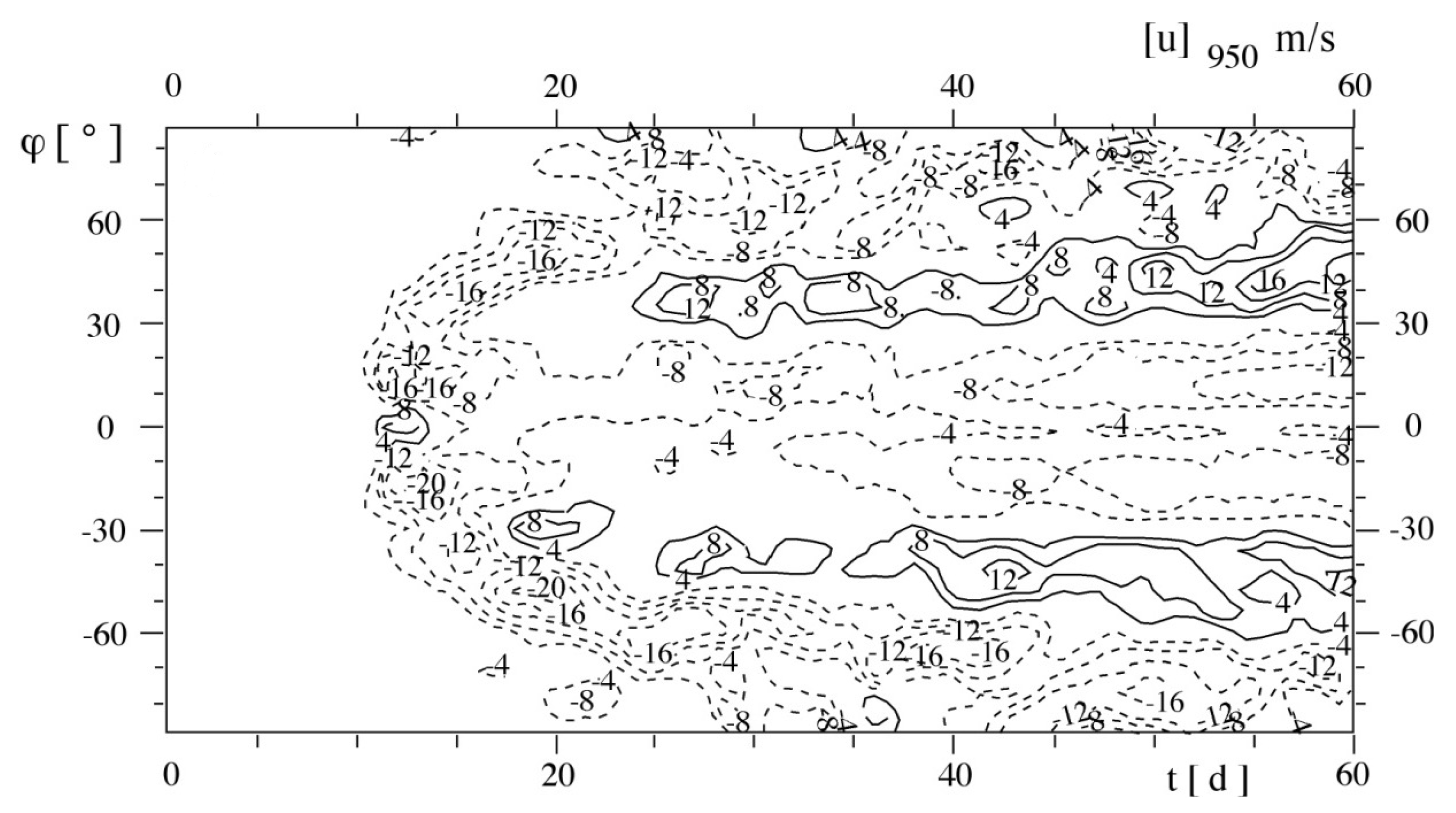
Figure 1. Fischer’s numerical experiment [5] running an atmospheric general circulation model of an aqua-planet Earth with an initial atmospheric state at rest. The shown variable is zonally averaged zonal wind at 950 hPa.
Atmosphere 15 01317 g001
Figure 2. Satellite image of small-scale features in the Northern Baltic Proper captured on 11 July 2005 [16].
Atmosphere 15 01317 g002
Figure 3. Locations where bottles, released into the Baltic Sea at the same place (see star off Bornholm) and at the same time, were eventually found after drifting through the Southern Baltic Sea [26]. Note that the bottles were not only moved by the currents but also by the wind.
Atmosphere 15 01317 g003
Figure 4. (Left): Analysis of river levels and groundwater levels in the 19th century, as prepared by Eduard Brückner (no units given) [27]. (Right): Proposition of the temporal spectrum of climate variability, as sketched by J. Murray Mitchell [28]. Used with permission from Cambridge University Press.
Atmosphere 15 01317 g004
Figure 5. Auto-correlation function (left) and auto-spectrum (right) of an AR(1) process with α = 0.3 and α = 0.5 . In the diagram with the spectra, white noise is also added as a horizontal line. From [38].
Atmosphere 15 01317 g005
Figure 6. Logarithm of daily variances of sea surface height in the SCS simulated for summer (top: gi) and winter (bottom: jl) by the low-resolution near-global model (left: g,j), the mid-resolution West Pacific model (middle: h,k), and the high-resolution South China Sea model (right: i,l). From [19].
Atmosphere 15 01317 g006
Figure 7. S/N ratios of zonal and meridional surface currents for the Bo Hai and Yellow Sea for (a) large-scale EOFs, (b) mid-size EOFs, and (c) small-scale EOFs. From [21].
Atmosphere 15 01317 g007
Figure 8. Noise levels vs. spatial scales in the numerical experiments, with and without tides, in the South China Sea. Note that the small scales are on the right. From [22].
Atmosphere 15 01317 g008
Figure 9. Memory vs. spatial scales in the numerical experiments, with and without tides, in the South China Sea. Note that, deviating from Figure 8, the large scales are on the left. From [22].
Atmosphere 15 01317 g009
Figure 10. Time series of standard deviations of the time series anomalies (i.e., deviations from the daily means of each ensemble) of atmospheric temperature (top; [43]) and oceanic depth-averaged velocity (bottom; [41]) at a grid point.
Atmosphere 15 01317 g010
Figure 11. Depth changes in an idealised model area after 240 years of integration, initialised at rest and exposed to slightly disturbed tides during the first 10 days [44].
Atmosphere 15 01317 g011
Figure 12. Integration of an energy-balance model with nonlinear albedo (cold temperatures go with a high albedo, low temperature with high albedo). (a) Development from different initial states, ending up in one of two stable states. (b) Integration when the transmissivity (for instance, by random variations in cloudiness) is considered random. Then, the system meanders between the two preferred states, and the frequency distribution becomes bimodal. The diagram is taken from [45] with permission from Springer Nature.
Atmosphere 15 01317 g012
Figure 13. Sensitivity of the formation of the spring cold water circulation in the western Yellow Sea to the presence of tides (left) and the presence of seasonal variations of wind stress (right). Three ensembles of simulations with full forcing (tides and wind), disregarding tidal forcing and disregarding the annual march of wind stress. Those points, at which a local t-test indicates the presence of a signal, are marked with a cross. The diagram is taken from [33].
Atmosphere 15 01317 g013
Disclaimer/Publisher’s Note: The statements, opinions and data contained in all publications are solely those of the individual author(s) and contributor(s) and not of MDPI and/or the editor(s). MDPI and/or the editor(s) disclaim responsibility for any injury to people or property resulting from any ideas, methods, instructions or products referred to in the content.