Lisbon Urban Climate: Statistical Analysis/Approach for Urban Heat Island Effect Based on a Pioneering Urban Meteorological Network

Abstract

The urban heat island (UHI) effect is a widely recognized phenomenon consisting of heat accumulation by dense urban construction and human activities, resulting in higher temperatures across urban areas compared to their surroundings. This article aims to quantify the UHI effect on several areas throughout the city of Lisbon, Portugal, with the main goal of validating, evaluating, and reinforcing urban climate adaptation and resilience strategies proposed in the recent scientific literature. A set of nine quality-controlled weather stations from the “Lisboa Aberta” network that are compliant with the World Meteorological Organization (WMO) standards and installation requirements were used to characterize Lisbon’s UHI, in comparison to a reference weather station from the Instituto Português do Mar e da Atmosfera (IPMA), located at Lisbon Airport. By applying a principal component analysis (PCA) in an innovative way to 10 urban indexes, it is shown that the thermal inertia in Lisbon’s urban areas is positively correlated with the UHI intensity and urban density, regardless of the daily heating/cooling cycle. Furthermore, the results show that land use also has an impact on the UHI effect, with continuous, vertical building areas showing the greatest deviations in comparison to the reference, averaging +1.8 °C. Contrastingly, horizontal building areas reveal an average deviation of +1.3 °C, with sparse, discontinuously built areas representing an average UHI effect of +0.2 °C. Finally, through a climatope analysis, it is determined that, across Lisbon, high-density urban areas and ventilation corridors are responsible for inducing average UHI effects of +1.7 °C and +0.2 °C, respectively.

1. Introduction

Both civil society and the scientific community are increasingly concerned about the risks posed by the growing frequency of heat waves and other extreme heat events. These risks, when combined with the urban heat island effect and climate change, significantly impact thermal comfort in cities, leading to clear consequences for public health [1,2,3,4].

Lisbon’s climate is temperate, with mild winters and precipitation mostly occurring between October and April. The hot season corresponds to the dry summer, classified as Csa under the Köppen climate classification system. The city’s climate is heavily influenced by topography, proximity to the Atlantic Ocean, and the Tagus Estuary [5,6,7].

Wind patterns show a high frequency and predominance of north and northwest winds, with considerable variability throughout the year [8,9]. During winter, wind directions fluctuate widely, while in summer, north to northwesterly winds (sea breezes) dominate around two-thirds of the afternoons and can prevail throughout the entire day on about 45% of days [10]. These winds, colloquially known as “nortada” [11,12], disperse accumulated heat, both natural and anthropogenic [13], and improve air quality by dispersing atmospheric pollutants.

Green spaces near residential areas positively impact human health by reducing pollution, improving air quality, and mitigating the urban heat island (UHI) effect [6,14,15]. The UHI effect, characterized by higher average air temperatures in urban areas compared to rural ones, significantly affects people’s quality of life in mid-latitude cities, especially during heat waves or extreme heat events. Urbanization exacerbates the UHI effect, negatively impacting thermal comfort and health, particularly in Southern Europe [4,16,17]. The UHI effect stems from the accumulation of solar energy in urban materials, driven by factors such as a low albedo, a high urban density, narrow streets (H/W index), a reduced sky view factor, a scarcity of green spaces and water, and anthropogenic heat sources [18]. Human activities in urban areas influence local temperature and wind, and urban climates result from changes these surfaces, materials, and activities cause in energy, mass, and movement balances [19,20].

Urban expansion leads to territorial changes, altering surfaces and, consequently, radiative and energy balances [21,22,23]. These changes modify topography and urban geometry, which strongly influence key radiative (solar and infrared) and energetic inputs and outputs (turbulent flows of sensible, latent, and stored heat). These factors were identified as primary causes of the UHI effect [21]. This phenomenon creates a thermal pattern with higher air and surface temperatures in cities than in adjacent areas, particularly at night. It forms a concentric thermal pattern, integrating all microclimates generated by urbanization [21,23,24,25]. UHI intensity (ΔTu-r) can be defined by the greatest temperature difference between a city (u) and its surroundings (r), ideally rural areas. It can also be compared to the lowest temperature of all rural-like areas surrounding a city at a given time [8,21,26,27], influenced by land use, urban morphology, and atmospheric and geographic conditions [28]. Addressing these factors is crucial for improving urban thermal comfort and public health [29].

Local climate zones (LCZs) and climatopes are key concepts in urban climate studies, differing primarily in their definitions, scope, and applications. LCZs provide a standardized classification of urban and rural areas based on local climatic characteristics [30]. They focus on physical and land use parameters influencing the urban microclimate, such as building height, vegetation cover, surface materials, and water bodies. The LCZ system includes 17 main zones, covering both dense urban and rural areas, and is particularly useful for comparing urban climates globally and studying phenomena like the UHI effect [24,31,32,33,34,35]. This standardization facilitates consistent data sharing and comparative studies worldwide [25]. In contrast, climatopes refer to homogeneous climatic areas within an urban region, defined by a mix of climatic, geographic, and anthropogenic factors, including topography, proximity to water bodies, building density, and human activities. Climatopes, being broader and less standardized than LCZs, focus on detailed microclimates within a city. They are often used for in-depth studies of climatic variations in different parts of a city, aiding local urban planning and environmental management [24].

This article analyzes the effect of urban indexes on temperature increases in specific locations within Lisbon, considering each area’s characteristics. The study focuses on the role of human actions in shaping the city’s physical space to improve the quality of life of its residents and visitors. It can be enlightening for the city council/municipality in the design and implementation of policy strategies, namely those of unconsolidated areas or areas under future urban planning projects, in order to improve thermal comfort in urban planning.

The paper’s main objective is to assess the urban environment’s quality in terms of thermal comfort, aiming to contribute to better spatial planning and a better understanding of the city’s urban climate (thermal) patterns. A difficulty encountered in this research was having a network shorter than it ideally would be, based on limitations related to the station data’s quality and/or availability. However, this study included more urban indexes than previous ones, using a total of 11 variables, which were subjected to a principal component analysis. A statistical analysis of the urban heat island effect is conducted, based on a pioneering urban meteorological network with nine strategically placed sensors across Lisbon’s seven parishes. The chosen locations are located within numerous climatopes, validating the previous views of relevant authors [35]. These chosen temperature sensors met the recommended quality standards, in terms of installation and data consistency. Additionally, the study seeks to investigate the following questions:

• Can climatopes be validated, reinforcing the measures proposed under the auspices of official literature [35] through UHI outputs?
• What is the direct influence of urban indexes (the net construction index, the implantation index, the open space index, the number of floors in the sensor area, the aerodynamic roughness index, the volumetry index, the compactness index, urban density classes, biomass (maximum annual value), and the sky view factor) on the UHI effect at each analyzed point in Lisbon, including the thermal inertia?
• How can decision makers promote and increase thermal comfort, as well as reduce the effects of the urban heat island in future urban planning?

2. Materials and Methods

2.1. Data Collection and Analysis Methodology

This chapter describes the methods for collecting, processing, and analyzing data, including our justification for choosing the areas studied, with a representation of the geographical location of each sensor addressed, as well as their general characteristics. In addition, we provide an overall criticism of the installation of these meteorological stations in light of good practice as promoted by the World Meteorological Organization (WMO). The methodology of analysis and statistical treatment as well as the linear regression and principal component analysis carried out in this work are also explained (Figure 1), including the differences between and approaches of all the variables used.

2.2. Chosen Areas and Neighborhoods

2.2.1. Justification for the Choice of Areas

The neighborhoods and meteorological stations addressed were chosen based on quality criteria for the installation of the sensors of the Lisbon Aberta network, from CML, having chosen, first, the meteorological stations with more rigorous or reasonable installation criteria, taking into account the limitations explained in Section 2.2.3. Within this first stage of filtering, we tried to choose cases that reflected the influence of physical (natural and anthropogenic) conditions on local temperature values, with special focus on urban density, ventilation, and land use characteristics. In this way, priority was given, within the existing possibilities, to stations with the best installation conditions, to those with the greatest possible range of data, and to holders of more constant and reliable records. Additionally, meteorological stations that were installed under different conditions within the same locality in terms of their urban indexes were prioritized for comparative purposes and to determine the influence of each of these indexes on the UHI effect. Meteorological stations were chosen in a very dispersed way in the municipality of Lisbon, with two main axes focusing on the areas of Ajuda and Parque das Nações/Beirolas, each of them composed by stations located in the same areas, but installed in areas with different land use classes, urban densities, and sky view factor values, among other differentiating criteria.

2.2.2. Geographical Location and General Characteristics of the Meteorological Stations of the Lisboa Aberta (CML) Network

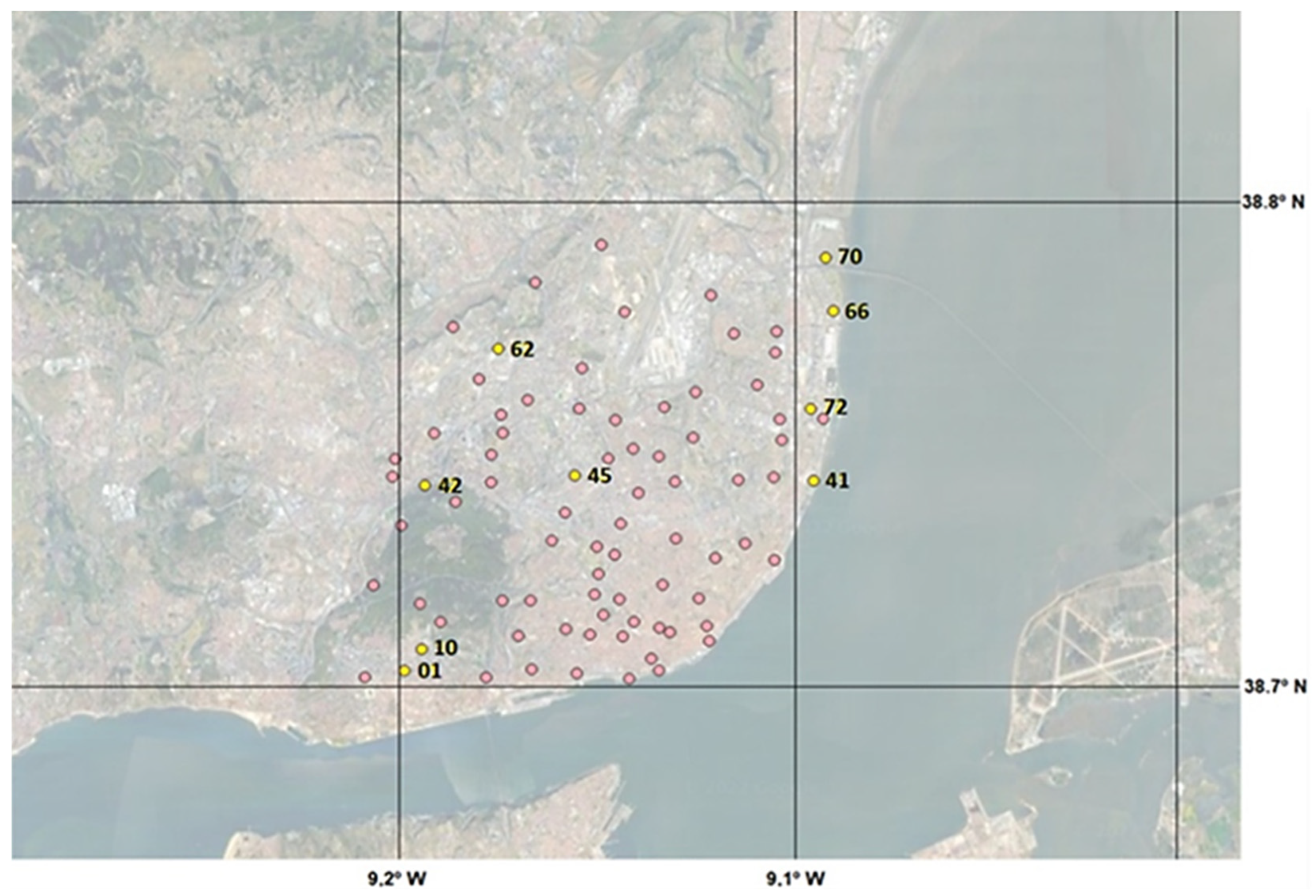
The sensors of the Lisboa Aberta network (Table 1) from the Câmara Municipal de Lisboa (CML) are dispersed throughout the municipality of Lisbon, with the sensors having been chosen for analysis in this dissertation highlighted in Figure 2.

As can be seen in Table 1, the chosen sensors are installed at very heterogeneous altitudes in the municipality of Lisbon, with the areas of Parque das Nações and Braço de Prata being the ones at the lowest altitude and with the area of Lumiar being at the highest altitude.

Table 1. Location of each sensor, altitude, and range of data used.

Station	Latitude (°)	Longitude (°)	Altitude (m)	Date (Start)	Date (End)
Sensor 01 Ajuda (Calçada da Ajuda)	38.7026	−9.1997	44	2 June 2021	31 December 2021
Sensor 10 Ajuda (Rua Sá Nogueira)	38.7111	−9.1951	95	1 June 2021	15 November 2021
Sensor 41 Jardim do Braço de Prata	38.7444	−9.0978	5	1 June 2021	1 December 2021
Sensor 42 Benfica (Travessa Francisco Rezende)	38.7434	−9.1943	90	12 July 2021	31 December 2021
Sensor 45 Entrecampos (Rua Frei Carlos)	38.7455	−9.1571	98	1 June 2021	25 December 2021
Sensor 62 Lumiar (Estrada do Paço do Lumiar)	38.7705	−9.1761	108	1 July 2021	20 December 2021
Sensor 66 Parque das Nações (Rua Ilha dos Amores)	38.7780	−9.0929	5	1 June 2021	31 December 2021
Sensor 70 Beirolas (Rua Chen He)	38.7885	−9.0948	4	1 June 2021	22 December 2021
Sensor 72 Limite Sul Parque das Nações (Rua. Mário Botas)	38.7586	−9.0985	26	14 June 2021	31 December 2021

Table 1. Location of each sensor, altitude, and range of data used.

Station	Latitude (°)	Longitude (°)	Altitude (m)	Date (Start)	Date (End)
Sensor 01 Ajuda (Calçada da Ajuda)	38.7026	−9.1997	44	2 June 2021	31 December 2021
Sensor 10 Ajuda (Rua Sá Nogueira)	38.7111	−9.1951	95	1 June 2021	15 November 2021
Sensor 41 Jardim do Braço de Prata	38.7444	−9.0978	5	1 June 2021	1 December 2021
Sensor 42 Benfica (Travessa Francisco Rezende)	38.7434	−9.1943	90	12 July 2021	31 December 2021
Sensor 45 Entrecampos (Rua Frei Carlos)	38.7455	−9.1571	98	1 June 2021	25 December 2021
Sensor 62 Lumiar (Estrada do Paço do Lumiar)	38.7705	−9.1761	108	1 July 2021	20 December 2021
Sensor 66 Parque das Nações (Rua Ilha dos Amores)	38.7780	−9.0929	5	1 June 2021	31 December 2021
Sensor 70 Beirolas (Rua Chen He)	38.7885	−9.0948	4	1 June 2021	22 December 2021
Sensor 72 Limite Sul Parque das Nações (Rua. Mário Botas)	38.7586	−9.0985	26	14 June 2021	31 December 2021

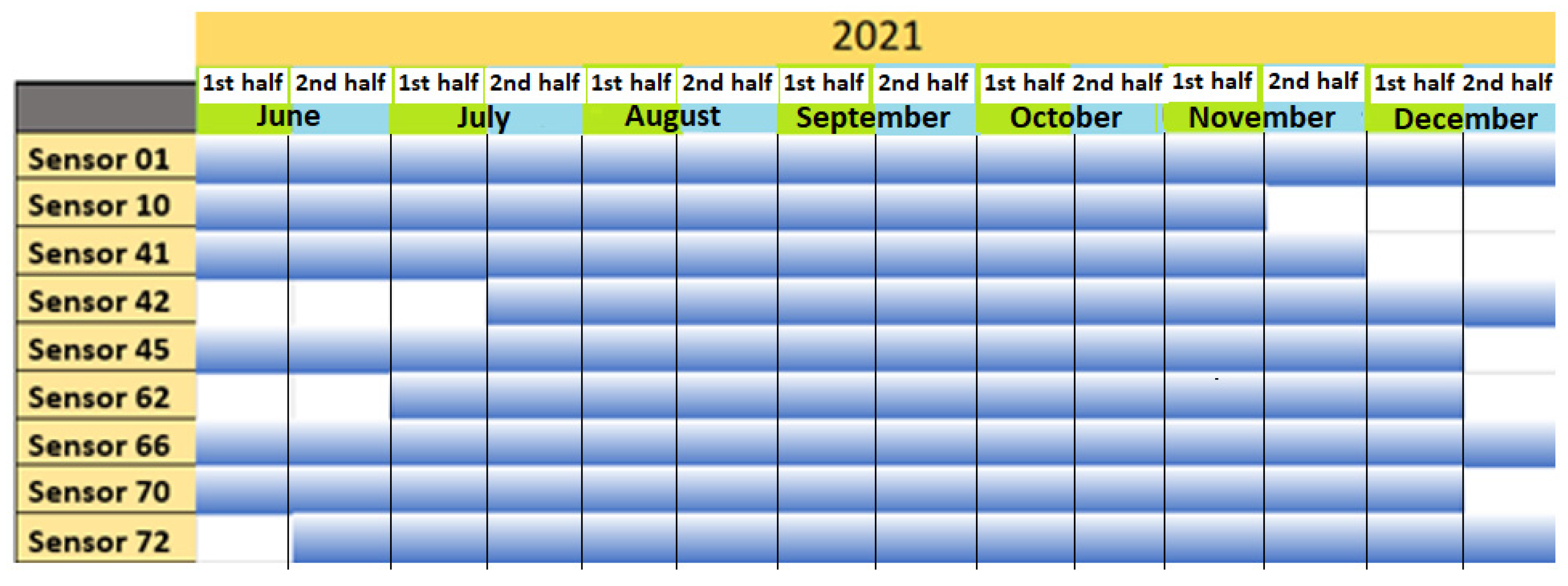
The scope of the data is quite satisfactory, with all the analyzed sensors at least having the period between the second half of July and the first half of November in common (Figure 3).

2.2.3. Critical Analysis of the Installation Conditions of Meteorological Stations in Light of the Good Practice Manual of the World Meteorological Organization (WMO)

To achieve the highest levels of accuracy and representativeness of air temperature measurements, thermometers must be shielded from both direct and diffuse solar radiation, whether originating from the sky, ground, or nearby structures or objects [36]. They must also be conveniently ventilated and exposed to the wind from all directions, so that there are no imbalances or asymmetries in the level of exposure for a fair comparison between different sensors. In regards to installation conditions, they must have an ideal standard installation height between 1.25 m and 2.00 m, as per the recommendations of good practice promoted by the World Meteorological Organization (WMO).

To adhere to the principle of radiation protection for sensors, the WMO recommends the following protective equipment:

(a)

Weather shelter (Stevenson shelter);

(b)

Meteorological shelter (composed of plates and radiation shield)

For weather shelters, it is critical that thermometers are not exposed to direct sunlight when the shelter door is open. Therefore, in the Northern Hemisphere, the door with shutters should open to the north, and in the Southern Hemisphere, to the south. This orientation minimizes direct solar radiation on the thermometers, although there might be a brief increase in exposure to diffuse solar radiation when the door is open.

In the case of the sensors installed on Lisbon’s streets, they were mounted at a height of approximately 3 m above ground. This placement was chosen to deter theft and overcome certain local installation challenges, which might influence their temperature readings, whose results were presented (Figure 4, Figure 5, Figure 6, Figure 7, Figure 8 and Figure 9). A notable deviation from WMO standards is the sensors’ proximity to surfaces like walls or vehicles (Figures S2, S4, S6, S8, S10, S12, S14, S16, and S18). These surfaces, often oriented towards the north or south, cause variations in ventilation and sun exposure due to the wind barrier effect created by buildings. Consequently, these factors may introduce inconsistencies in sensor comparisons, particularly concerning direct sunlight exposure times.

2.3. Acquisition of Data Used

Instrumentation, Data, and Software Used to Collect and Process Series

This study utilizes data collected from these sensors, acknowledging their specific limitations (Table 2). To enhance the quality of the final data, a rigorous quality control process was applied to the temperature data for each UTC hour. This process included the following:

• Filtering sensors to ensure consistent data quality;
• Removing outliers from the selected sensors [37];
• Synchronizing all sensor data with UTC time;
• Analyzing the temperature distribution for each sensor and determining the first and third quartiles, median, minimum, and maximum values [37].

Table 2. Instruments, meteorological data, other data, and software used, as well as their respective characteristics and uses.

	Type of Station	Characteristics	Uses
Instruments	Lisbon City Council weather stations	Wireless thermometers with 2G, 3G, and 4G communication Accuracy: ±0.5 °C and 0.1 °C resolution	Air temperature measurement
Weather data	Lisbon City Council weather stations	Hourly temperature data at each of the analyzed stations: sensors 01, 10, 41, 42, 45, 62, 66, 70, and 72	Extraction, filtering, and treatment of air temperature data series for measurement at fixed points and determination of the intensity of the UHI effect in each area
	Lisbon Airport meteorological station (LPPT)	Hourly data for temperature, cloud cover, and wind strength and direction	Use of temperature data as a regional reference to determine the intensity of the UHI effect at each of the remaining points analyzed. Use of data on cloud cover and wind intensity and direction as a regional reference, according to official methodology [35]
Other data	Information on morphology and other urban characteristics	Net construction index Implantation index Open space index Number of floors in the sensor area (within 100 m of the corresponding street) Aerodynamic roughness index Volumetry index Compactness index (H/W) Urban density classes Biomass (maximum annual value) [15] Sky view factor	Estimation of the relationship between each of the urban parameters and morphological characteristics of the city with the UHI effect of each location
Software	Python Scripts 3.12		Extraction and processing of data from Lisbon Aberta sensors from CML
	QGIS, version 3.16.4		Extraction of values at each chosen point to be associated with the urban characteristics of the location of each sensor
	RayMan Pro 3.1 Beta		Construction of solar diagrams for each sensor to calculate the SVF
	SunEarthTools v3.0		Construction of solar diagrams referring to each sensor, combined with the RayMan Pro software, in order to quantify hours of solar exposure and angles of solar incidence on the street surfaces in each of the seasons.
	Surfer v9		Conversion of data displayed originally in a table into a coloured-map, transforming the x-axis in longitude and y-axis in latitude values, showing the horizontal distribution of UHI effect.
	SPSS Statistics v26		Statistical treatment of extracted data

Table 2. Instruments, meteorological data, other data, and software used, as well as their respective characteristics and uses.

	Type of Station	Characteristics	Uses
Instruments	Lisbon City Council weather stations	Wireless thermometers with 2G, 3G, and 4G communication Accuracy: ±0.5 °C and 0.1 °C resolution	Air temperature measurement
Weather data	Lisbon City Council weather stations	Hourly temperature data at each of the analyzed stations: sensors 01, 10, 41, 42, 45, 62, 66, 70, and 72	Extraction, filtering, and treatment of air temperature data series for measurement at fixed points and determination of the intensity of the UHI effect in each area
	Lisbon Airport meteorological station (LPPT)	Hourly data for temperature, cloud cover, and wind strength and direction	Use of temperature data as a regional reference to determine the intensity of the UHI effect at each of the remaining points analyzed. Use of data on cloud cover and wind intensity and direction as a regional reference, according to official methodology [35]
Other data	Information on morphology and other urban characteristics	Net construction index Implantation index Open space index Number of floors in the sensor area (within 100 m of the corresponding street) Aerodynamic roughness index Volumetry index Compactness index (H/W) Urban density classes Biomass (maximum annual value) [15] Sky view factor	Estimation of the relationship between each of the urban parameters and morphological characteristics of the city with the UHI effect of each location
Software	Python Scripts 3.12		Extraction and processing of data from Lisbon Aberta sensors from CML
	QGIS, version 3.16.4		Extraction of values at each chosen point to be associated with the urban characteristics of the location of each sensor
	RayMan Pro 3.1 Beta		Construction of solar diagrams for each sensor to calculate the SVF
	SunEarthTools v3.0		Construction of solar diagrams referring to each sensor, combined with the RayMan Pro software, in order to quantify hours of solar exposure and angles of solar incidence on the street surfaces in each of the seasons.
	Surfer v9		Conversion of data displayed originally in a table into a coloured-map, transforming the x-axis in longitude and y-axis in latitude values, showing the horizontal distribution of UHI effect.
	SPSS Statistics v26		Statistical treatment of extracted data

2.4. Analysis and Statistical Treatment Methodology, Linear Regression, and Principal Component Analysis

2.4.1. Variables under Study

The data analyzed in this study refer to meteorological variables (

Table 3. Variables under study and respective descriptions.

Variable	Comments
Average temperature deviation value	Dependent variable. Difference between each sensor and the reference station. Average of the entire period.
Net construction index	Independent variable. The building index establishes the relationship between the building area and the land area on which the operation is based. It is expressed by the formula (ic) i = ΣAj/S.
Implantation index	Independent variable. The implantation index establishes the relationship between the implantation area of the buildings and the area of land that serves as the base for the operation, expressed in %. It is expressed by the formula p = (A0/S) × 100.
Open space index	Independent variable. The open space index is the inverse of the building index. It is expressed by the formula 1/ic.
Number of floors in the sensor area	Independent variable. Determines the average number of floors that make up the buildings on the street where the sensor is located over a 100 m distance, rounded to the nearest unit.
Aerodynamic roughness index	Independent variable. Aerodynamic roughness (Z0) is a morphometric index that evaluates surface friction.
Volumetry index	Independent variable. The volumetry index relates the volume of existing buildings in a given area (of 100 × 100 m) to the average volume if the cell was fully occupied. It is expressed by the formula (IV) iv = Σ Vj/S.
Compactness index (H/W)	Independent variable. This index establishes the ratio between the height of buildings (H) and the width of streets (W).
Urban density classes	Independent variable. Urban density classes reflect a relationship between aerodynamic roughness (Z0), compactness index (H/W), and volumetry index (I/V), among other components derived from these.
Biomass (maximum annual value)	Independent variable. Adapted from published methodology [15], according to the methodology recommended by the author for the city of Lisbon, expressed in kg/m2. Presence of biomass (kg/m2) = 0.148 + 1.735 × NDVI, a formula that was previously adapted [38]
Sky view factor (SVF)	Independent variable. The SVF value reflects the urban geometry of the respective point where it is located, ranging from 0 (zero) to 1, with the value of 1 corresponding to an area without any obstacle that comes between the chosen point and the sky. An SVF of 1 (no obstructions) under clear-sky conditions, receives shortwave radiation all day and emits longwave radiation at night. Different FVC values mean different radiative balances and therefore different energy stores.

), urban indexes, and morphological parameters for each analyzed location from a temperature, speed, and wind direction database covering daily records from the period from 1 June to 31 December 2021.

2.4.2. Selection of Meteorological and Urbanistic Variables

The data analyzed in this study refer to meteorological variables, urban indexes, and morphological parameters for each analyzed location from a temperature, speed, and wind direction database covering daily records from the period from 1 June to 31 December 2021.

Statistical variables can be of several types: categorical or qualitative (which include nominal and ordinal), quantitative (discrete or continuous), and ordinal. Selection of Meteorological and Urbanistic Variables has the following main objectives:

• Identification, selection, and treatment of meteorological, morphological, and urban variables representative of the municipality of Lisbon;
• Creation of a typology of temperature patterns, based on the identification of main components and cluster analysis.

Our selection of variables was intended to capture the interrelationships between temperature, as a dependent variable, and elements correlated with a greater or lesser UHI effect, given the implications of the morphology of the city and the urban indexes of each point analyzed to determine the thermal behavior of each location. In addition, our approach to the temperature-dependent variable separates daytime and nighttime periods based on official methodology [9], in which the daytime period was considered to be between 10:00 and 18:00 and the nighttime period was considered to be between 20:00 and 06:00 the following day, inclusively. Thus, the possible influence of twilight transition periods on air temperature patterns at each location is excluded. While the temperatures extracted from the Lisbon City Council database were strictly quality-controlled, the remaining independent variables were considered as is.

2.4.3. Main Component Analysis

Principal component analysis (PCA) is a multivariate exploratory analysis technique that transforms a set of correlated variables into a smaller set of independent variables, linear combinations of the original variables called principal components. This method of analysis allows us to reduce the complexity of the data and summarize the information of correlated variables as one or several independent linear combinations [37]. The selection of variables is intended to capture the interrelationships between temperature, as a dependent variable, and elements correlated with a greater or lesser UHI effect, given the implications of the morphology of the city and the urban indexes of each point.

2.4.4. Model Summary

Initially, a PCA was performed for the 11 (n − 1) variables under study, as per the criteria of the Kaiser method, and later the dimensions with eigenvalue greater than 1 were filtered, whereby part of the information on all of the samples was deleted, resulting on 72.7% of the temperature variability (dependent variable) which can be explained by the present model, which is a relatively robust number (Table 4).

The explained variance (Table 5) makes it possible to describe the variance of each of the original variables in the new main components (dimensions) either in terms of the centroids (i.e., the mean scores for each individual registered in that variable) or in terms of the total (the coordinates’ eigenvectors) [37]. This measure allows us to understand which variables are decisive for each of the principal components. In the loading component matrix (Table 6), those that present a loading value greater than at least 0.5 are accepted as determining absolute variables (as marked in Table 7).

2.4.5. Loading Components

Official literature [37] states that formality is opposite to the intensity and frequency of interaction, meaning that in the loading components, those that present a loading at least greater than 0.5 in value are accepted as determining absolute variables (marked in Table 7). After selecting the loadings, it will be possible to understand what defines each component. In principal component analysis (PCA), identifying variables with loadings greater than 0.5 is crucial because these loadings indicate the strength and direction of each variable’s contribution to a principal component. A loading greater than 0.5 suggests that the variable has a significant impact on the component, helping to define its meaning.

These variables are essential for interpreting each component because they reveal which underlying factors are most influential in shaping the data structure. In the context of this study, components might represent different aspects of UHI patterns, such as construction rate, aerodynamic roughness, compactness index (H/W), volumetry index, and sky view factor. By focusing on variables with loadings above 0.5, it is more accurate and easy to characterize each component, ensuring that the analysis captures the most significant factors driving thermal variations in Lisbon. This approach leads to a more robust understanding of the data and supports the development of strategies for mitigating UHI effects.

2.4.6. Cluster Analysis

In this study on thermal patterns in Lisbon, hierarchical clustering is chosen due to its ability to identify natural groupings within the data without needing a prior assumption about the number of clusters. This method is particularly useful for complex urban environments where patterns may not be easily defined. Hierarchical clustering allows for a detailed analysis by progressively merging individual points or clusters, enabling researchers to observe how thermal patterns group together at various levels of similarity.

Cluster analysis is a multivariate exploratory technique that allows for the grouping of subjects or variables into homogeneous groups with one or more common characteristics. Each observation belonging to a given cluster is similar to all others belonging to that cluster and is different from observations belonging to other clusters [37]. It is possible to perform cluster analysis using similarity measures or dissimilarity measures (distance). This analysis was developed using the hierarchical clustering technique, in which the variables are first aggregated and then grouped according to their proximity [37].

The “greatest distance” method, also known as the complete linkage method, was selected because it is particularly effective in creating compact and well-separated clusters. This approach considers the maximum distance between any two points in different clusters during the merging process, which tends to produce clusters that are more distinct from each other. In the context of urban heat island (UHI) effect in Lisbon, this method ensures that areas with significantly different thermal characteristics are not grouped together prematurely, thus preserving the integrity of the thermal patterns being studied.

There are seven proximity calculation methods; however, for the present study, only 3 fit: shortest distance, greatest distance, and average distance between clusters. Taking into account the results obtained through the three methods, the one with the greatest distance (the most distant neighbor) was the most interesting, which ended up being the one that continued the analysis. Through the agglomeration of clusters by the nearest neighbor method, the number of clusters to result from this analysis is also defined. After obtaining a dendrogram (graph that allows for the simplification of information, allowing us to better visualize the formed clusters), it was necessary to proceed to cut it, in order to individualize the clusters.

The formula used for this purpose was as follows (1):

K = 1 + 3.3 log n.

(1)

In the formula, n is the number of units of analysis, that is, in this case, the total number of CML meteorological stations under study × 2 (daytime and nighttime); therefore, it was 18 (9 meteorological stations × 2 daily periods).

If n = 18, then the following is obtained:

K = 1 + 3.3 log 18 = 5.14

(2)

That is, in order to create correct output boxplots (see Figure 9 later on) and to obtain 5 clusters (see Figure 10 later on) the cut in the dendrogram must be made.

This formula is used to determine the optimal number of clusters for analysis. Applying this formula ensures that the clustering solution is neither overly simplistic nor excessively complex, which is crucial for meaningful interpretation.

For UHI patterns, the number of clusters directly influences how these patterns are categorized and understood. By determining K using this formula, the analysis is guided towards a solution that balances detail with generalization. Too few clusters might oversimplify the diversity of thermal patterns, while too many could result in overfitting, in which the clusters represent noise rather than meaningful groupings. Therefore, using this formula helps in identifying a number of clusters that provide a clear and insightful understanding of how thermal characteristics vary across different areas of Lisbon, leading to more accurate conclusions.

2.4.7. Data Collection and Quality Control

Air temperature data were taken from each of the 9 chosen sensors from the Lisboa Aberta network from the Municipality of Lisbon (CML). Outliers were identified and removed based on the interquartile range (Q3–Q1), with the lower and upper limits determined using Equations (3) and (4) as follows:

$$(\mathrm{L}\mathrm{I}\mathrm{n}\mathrm{f}=\overline{x}-1.5\times \mathrm{I}\mathrm{Q}\mathrm{R})$$

(3)

$$(\mathrm{L}\mathrm{S}\mathrm{u}\mathrm{p}=\overline{x}+1.5\times \mathrm{I}\mathrm{Q}\mathrm{R})$$

(4)

This procedure aimed to compare the temperature deviations of each sensor, both during the day and at night, against the Lisbon Airport meteorological station (LPPT), which serves as the regional reference. This approach enabled the creation of the aforementioned boxplots (Figure 9), which visually depict the interquartile range and median for each sensor analyzed, distinguishing between daytime and nighttime readings. Other stations were excluded from the study due to their poor installation quality and data gaps, which hindered accurate and consistent comparisons between the different sensors. For temperature, wind, and cloud cover data, hourly readings from the Lisbon Airport meteorological station (LPPT) were used. These data were synchronized with the meteorological stations under study, ensuring the reference time was UTC. This time standard allows for reliable comparisons throughout the year, even during the transition to winter, which occurs on the last Sunday of October each year (in 2021, this occurred at 2:00 a.m. on 31 October).

To examine the influence of urban density and physical characteristics of each location, whether natural or anthropogenic, this study focused on selecting the maximum number of sensors within the same location. This approach facilitated comparisons while prioritizing the quality of sensor installation as the initial filtering criterion. Following this stage, a comprehensive analysis of Lisbon was conducted, alongside a focused study of two specific areas: Ajuda (sensors 01 and 10) and Parque das Nações/Beirolas (sensors 66, 70, and 72). These analyses aimed to investigate temperature differences observed over short distances within the same parish, exploring potential causes. The selected stations, despite being relatively close and within the same parish, are situated in areas that are heterogeneous in terms of urban and topographical features, as well as natural ventilation. The thermoisopleth maps (Figure 11) and axes chosen (Figure 12 and Figure 13) highlight the topographical features of each parish, with cross-sectional profiles running northeast–southwest in Ajuda and north–south in Parque das Nações/Beirolas, illustrating the exposure of each sensor.

The filtering and correction of temperature data collected from the CML’s Lisboa Aberta network sensors involved eliminating outliers. This process was based on calculating the interquartile range (Q3-Q1) and determining the lower (Equation (3)) and upper (Equation (4)) limits when comparing temperature deviations, whether during the day or at night, for each sensor against the Lisbon Airport meteorological station (LPPT). This technique also facilitated the creation of boxplots (Figure 9), visually representing the interquartile range and median of each analyzed sensor for both daytime and nighttime components. A Python script was developed to handle missing hourly data by leaving them blank. Additionally, the data validation procedure, based on a synchronous comparison with the Lisbon Airport reference station (LPPT), enabled the identification of behavior patterns for each sensor in relation to the reference. This process helped to identify significant deviations from expected thermal patterns, allowing outliers to be flagged. The results, expressed as hourly air temperature differences (Δ), are presented graphically, providing a clearer analysis of the thermometric patterns at each analyzed point compared to the reference station. Removing outliers has some implications, with data availability/reduction being one of them. This was the preferred method [37] as it allowed us to preserve only higher-quality data, even if it led us to have fewer temperature (UHI) data. The original data were full of questionable values which needed to be filtered. This method is a usual and safe practice in this type of data analysis.

2.5. Mapping of Outputs

The outputs produced are presented in tables and graphs, with the aim of representing the results obtained in a more visual way for each of the analyzed cases. Additionally, the procedures used for this purpose are listed.

2.5.1. Mapping of the UHI Effect Based on the Chosen Sensors

UHI effect presents a thermal pattern in which there are higher air and surface temperatures in cities than in adjacent areas, with the night period therefore showing a concentric thermal pattern. The integration of all microclimates due to the urbanization process and its intensity (ΔTu-r) can be defined as the greatest difference verified between the temperature of the city (u) and the temperature of its surroundings (r), ideally countryside. It can also be compared with the lowest temperature of all places with rural characteristics that surround the city at a given moment [8,21,26,27], which may occur according to the characteristics of land use and urban morphology, as well as atmospheric and geographic conditions [28]. Given this, the methods of relevant publications were followed and the most similar weather station (in terms of the aforementioned conditions) was taken into account, which was the official weather station of Lisboa Portela (LPPT) from Portuguese Institute for Sea and Atmosphere.

Based on the points mentioned earlier, data collected from the CML’s Lisboa Aberta network database were considered and subsequently inserted into Surfer v9 software. Surfer software was used to transform data displayed originally in a table into a coloured map, transforming the x-axis for longitude values and y-axis for latitude values. In this way, a map was created that shows the horizontal distribution of UHI effect. The z value corresponds to the UHI value at each point, enabling a patch and isoline distribution in this graphical output. Regarding the temperature distribution maps and altitude, obtained through a vertical section of the atmosphere at each location, the x-axis represents the altitude, while the y-axis indicates the time (UTC) of each observation. The z value reflects the intensity of the UHI effect at each point, measured hourly on 10 July 2021, selected as one of the hottest days of that particular year.

The identification of these air temperature patterns followed the methodology outlined below:

(a)

The comparison of the collected data considered the temperature difference between the thermometric stations and the reference station, Lisboa Portela (LPPT). The reference station, located at the highest altitude (104 m), reflects the behavior closest to the regional meteorological situation and furthest from the anthropogenic effects of urban density. Positive temperature differences indicate that the thermometric stations record higher temperatures than the reference station, and the opposite is true when the differences are negative;

(b)

To identify patterns, two periods were selected (daytime and nighttime), following the methodology discussed earlier, which has been employed by other authors [9]. The daytime period includes the time between 10:00 and 18:00, while the nighttime period refers to the time between 20:00 and 06:00 the following day. The objective is to encompass the lowest and highest daily values possible, excluding twilight periods according to the aforementioned methodology;

(c)

The classification of daily periods was conducted by individualizing each hour, allowing for the grouping of observations into different categories for the production of maps with vertical sections and the analysis of the altitudinal temperature pattern in each study area (despite the lack of a height effect above the ground, as all sensors are positioned 3 m above the ground, though at different altitudes relative to mean sea level). These thermoisopleth maps (showing altitude factor and maintaining the same height above the ground) use the following variables: altitude, temperature, and time (UTC hours). To understand the influence of various urban indexes, it is recommended to consult Figures S19–S29, which detail the physical conditions, whether natural or anthropogenic, at each sensor’s installation site;

(d)

The production of cross-sections along the study areas’ axes, in the NE–SW direction (Ajuda) and North–South (Parque das Nações/Beirolas), enables the verification of air temperature distribution patterns at each UTC hour on 10 July 2021, for each sensor in the parishes of Parque das Nações/Beirolas and Ajuda. This day was selected because it was one of the hottest days of the year 2021, characterized by predominantly clear or slightly cloudy skies, thus allowing for greater energy accumulation on various surfaces and materials. The aim was to study one specific day in order to show the thermal performance/patterns of each axis. So, to do that, a day in which thermal stress occurred was chosen in the hope that it would provide meaningful results in our analysis.

2.5.2. Classification of UHI Intensities

Data collected from CML’s Lisboa Aberta database and the hourly air temperature differences (Δ) between each sensor and the Lisbon Airport reference station (LPPT) were considered. These differences were represented based on the division of the data of each sensor into 6 classes: values below −4 °C, values between −4 °C and −2 °C, values between −2 and 0 °C, values between 0 °C and 2 °C, values between 2 °C and 4 °C, and values above 4°C.

3. Results

3.1. General Results

The location of each sensor and its physical characteristics, whether natural or anthropogenic, strongly affected the temperature values obtained, given that areas characterized by high levels of urban density, compactness, aerodynamic roughness, and soil impermeability have a greater impact on the local climate, as opposed to rural and semi-rural areas, which have a smaller presence of buildings and a greater presence of permeable soils and vegetation, shrubs, or trees (Figure S20). Therefore, a strong anthropic influence is expected on the temperature values measured in places with a greater urban density.

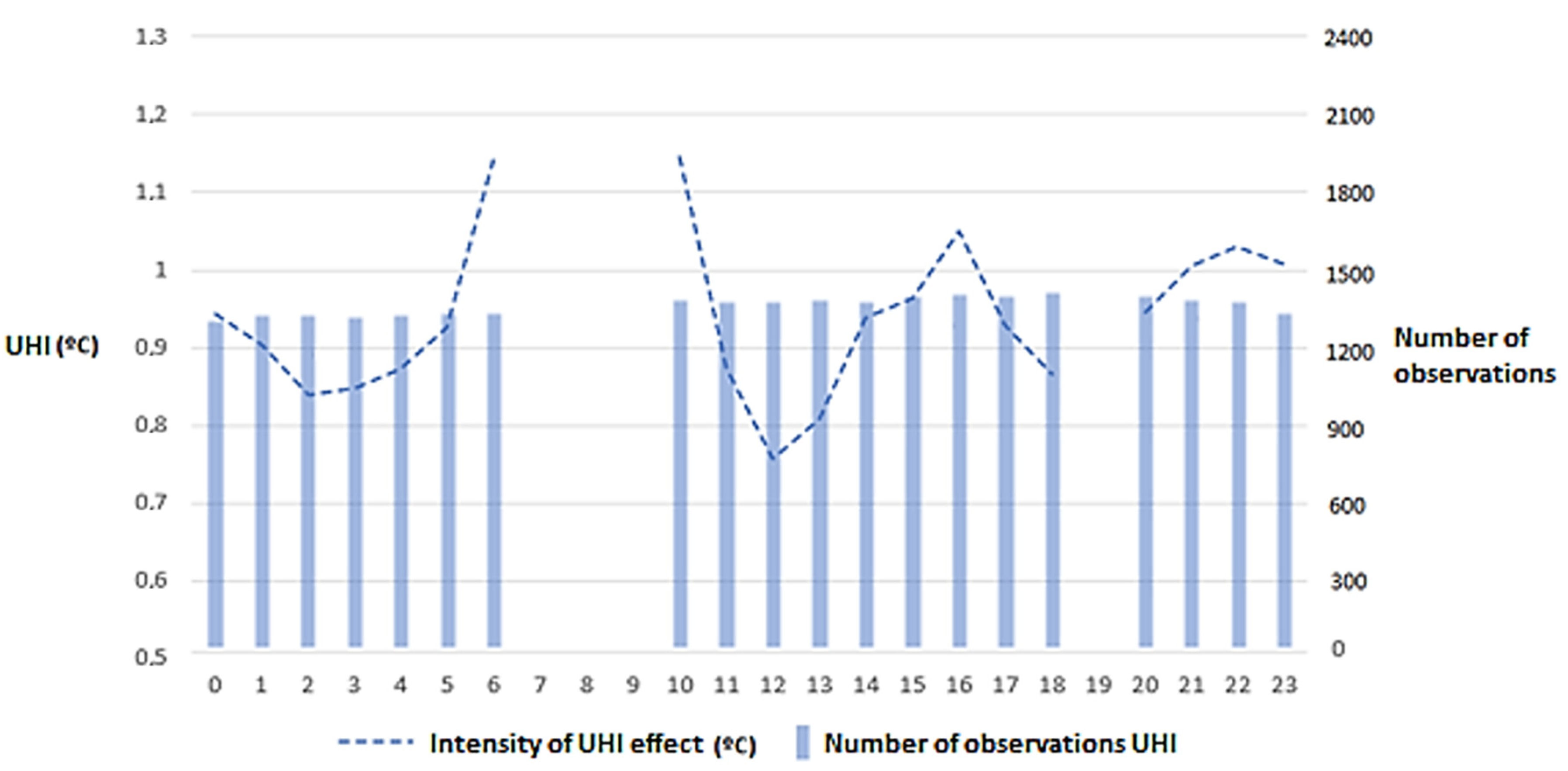
The UHI effect was more intense on average (for all the analyzed sensors) between 6:00 UTC and 10:00 UTC. There were some higher values between 20:00 and 00:00 UTC, after which there was a gradual reduction in the difference between the values and those of the meteorological station of Lisbon Airport (LPPT). In contrast, the period between 11:00 UTC and 14:00 UTC is the one in which the UHI effect is weakest, taking into account the average of all sensors (Figure 4). However, some sensors behave differently, depending on the characteristics of the places in which they are installed (see Figures S19–S29). The number of temperature observations taken into account for each hour of analysis for this dissertation was quite homogeneous, with around an average of 1400 observations (Figure 4).

Figure 4. Number of observations used for each hour throughout the observed period and corresponding average UHI effect (average value of all sensors). Produced according to official methodology [9], leaving out twilight periods between 07:00 and 09:00 UTC, inclusively, and 19:00 UTC.

Figure 4. Number of observations used for each hour throughout the observed period and corresponding average UHI effect (average value of all sensors). Produced according to official methodology [9], leaving out twilight periods between 07:00 and 09:00 UTC, inclusively, and 19:00 UTC.

On average, the frequency of the UHI effect intensities was higher at night, with the (0 °C; 2 °C] UHI effect class having about 15% more occurrences at night than during the day. On the other hand, the (−2 °C; 0 °C] and (2 °C; 4 °C] classes have on average around 5% more occurrences during the day. Additionally, in the (−4 °C; −2 °C] class, occurrences during the daytime are about three times higher than occurrences during the night period (Figure 5, Figures S3, S5, S7, S9, S11, S13, S15, S17, and S19), verifying that the urban freshness island effect (UFI), when especially intense, tends to occur during the daytime period.

Figure 5. Relative daytime and nighttime frequencies regarding the local UHI effect for all the sensors studied.

Figure 5. Relative daytime and nighttime frequencies regarding the local UHI effect for all the sensors studied.

3.1.1. Main Component Analysis

The principal component analysis determined the emergence of five final dimensions, created from the 11 initial study variables that characterized the addressed theme. It was performed according to the criteria of the Kaiser method, maintaining the maximum possible variance explained with the smallest possible number of dimensions, determining the part of the variance to be discarded by filtering eigenvalues (the variance extracted by the component) greater than one only, and considering that part of the totality of the sample information is eliminated.

3.1.2. Model Summary

This model has an R of 0.852 and an R² of 0.727, which means that 72.7% of the temperature variability (dependent variable) can be explained by the present model, which is a relatively robust number (Table 4).

Table 4. Model summary.

R	R Square	Adjusted R Square	Std. Error of the Estimate	R Square Change	F Change	Sig. F Change	Durbin–Watson
0.852	0.727	0.487	0.542259	0.727	3.036	0.071	1.895

Table 4. Model summary.

R	R Square	Adjusted R Square	Std. Error of the Estimate	R Square Change	F Change	Sig. F Change	Durbin–Watson
0.852	0.727	0.487	0.542259	0.727	3.036	0.071	1.895

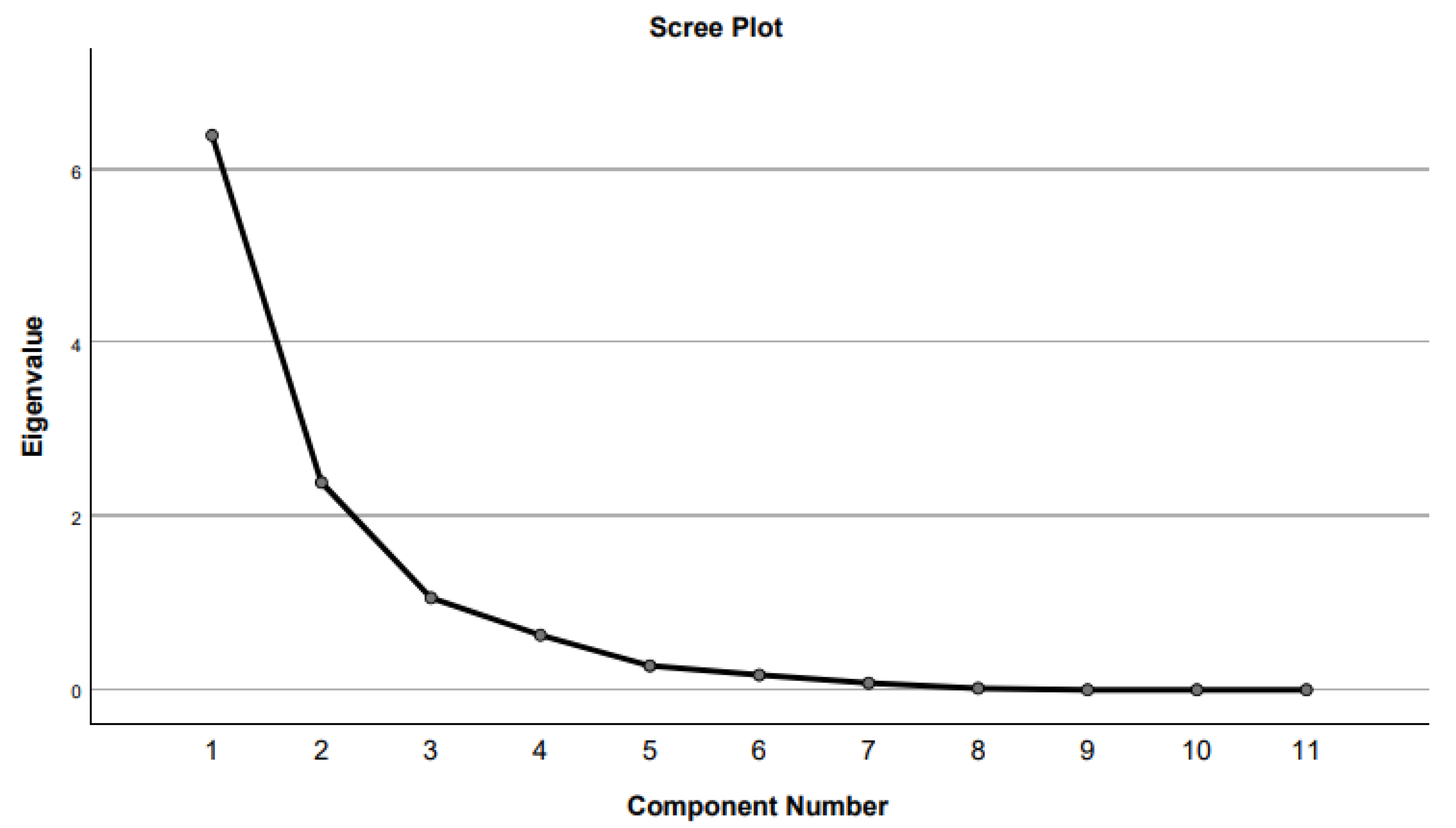
Figure 6 and Table 5 show the explanatory variance of each PCA dimension. The first dimension/component has an eigenvalue of 6.573, which corresponds to 54.77% of the total variance, which is the component that has the highest explanatory value of the total variance of the original variables. Then, the second component, with an eigenvalue of 2.415, which represents approximately 20.12% of the variance, explained the greater proportion of the variance not explained by the first component, which is independent. The third and last extracted component has an eigenvalue of 1.410, representing 11.75% of the variance. The remaining values have less weight in terms of the explanatory value of the original variables, since they have only residual values, all below 7%, and were not included as selectable main components, since they have eigenvalues below one. The three calculated dimensions represent approximately 86.65% of the original variables, and the first two components explain 74.90% of the total variance. All the analyzed variables were converted into their respective orders (by default), showing an apparently normal distribution [37].

Table 5. Variance explained by the model.

Component	Initial Eigenvalues
	Total	% of Variance	Cumulative %
1	6.573	54.774	54.774
2	2.415	20.124	74.898
3	1.410	11.747	86.645
4	0.747	6.228	92.873
5	0.422	3.513	96.386
6	0.237	1.976	98.362
7	0.171	1.423	99.785
8	0.026	0.215	100.000
9	1.681 × 10−9	1.400 × 10−8	100.000
10	7.082 × 10−16	5.902 × 10−15	100.000
11	7.810 × 10−17	6.508 × 10−16	100.000

Table 5. Variance explained by the model.

Component	Initial Eigenvalues
	Total	% of Variance	Cumulative %
1	6.573	54.774	54.774
2	2.415	20.124	74.898
3	1.410	11.747	86.645
4	0.747	6.228	92.873
5	0.422	3.513	96.386
6	0.237	1.976	98.362
7	0.171	1.423	99.785
8	0.026	0.215	100.000
9	1.681 × 10−9	1.400 × 10−8	100.000
10	7.082 × 10−16	5.902 × 10−15	100.000
11	7.810 × 10−17	6.508 × 10−16	100.000

Figure 6. Eigenvalue of each component determined in the principal component analysis.

Figure 6. Eigenvalue of each component determined in the principal component analysis.

The explained variance makes it possible to describe the “variance of each of the original variables in the new main components (dimensions) either in terms of the “centroids” (i.e., the mean scores for each individual registered in that variable) or in total terms (in terms of the coordinates eigenvectors)” [37]. This is a measure that allows one to understand which variables are decisive for each principal component.

3.1.3. Loading Component

Official literature [37] states that “formality is opposite to the intensity and frequency of interaction”, meaning that in the loading component (Table 6), those that present a loading value greater than at least 0.5 are accepted as determining absolute variables (as marked in Table 7).

Table 6. Matrix of model components.

Variable	Component
	1	2	3
Average_value_temp_dev	0.677	−0.015	0.228
Net_construction_index	0.893	0.005	−0.355
Implantation_index	0.592	−0.774	−0.211
Open_space_index	−0.592	0.774	0.211
Number_floors	0.633	0.411	0.581
Roughness index (Z0)	0.890	0.382	−0.080
Volumetry_index	0.426	−0.697	−0.509
Compactness_H/W_index	0.918	0.194	−0.271
Urban_density_classes	0.850	0.389	0.021
Maximum_biomass	−0.848	0.250	−0.305
Sky_view_factor	−0.876	−0.368	0.147

Table 6. Matrix of model components.

Variable	Component
	1	2	3
Average_value_temp_dev	0.677	−0.015	0.228
Net_construction_index	0.893	0.005	−0.355
Implantation_index	0.592	−0.774	−0.211
Open_space_index	−0.592	0.774	0.211
Number_floors	0.633	0.411	0.581
Roughness index (Z0)	0.890	0.382	−0.080
Volumetry_index	0.426	−0.697	−0.509
Compactness_H/W_index	0.918	0.194	−0.271
Urban_density_classes	0.850	0.389	0.021
Maximum_biomass	−0.848	0.250	−0.305
Sky_view_factor	−0.876	−0.368	0.147

Table 7. Model correlation matrix.

Variable	Average_Value_Temp_Dev	Net_Construction_Index	Implantation_Index	Open_Space_Index	Number_Floors	Roughness Index (Z0)	Volumetry_Index	Compactness_H/W_Index	Urban_Density_Classes	Maximum_Biomass	Sky_View_Factor
Average_value_temp_dev	1	−0.489	0.347	−0.347	0.391	0.507	0.343	0.522	0.665	−0.563	−0.490
Net_construction_index	0.489	1	0.583	−0.583	0.369	0.801	0.187	0.897	0.761	−0.698	−0.798
Implantation_index	0.347	0.583	1	−1	−0.052	0.258	0.685	0.464	0.180	−0.626	−0.274
Open_space_index	−0.347	−0.583	−1	1	0.052	−0.258	−0.685	−0.464	−0.180	0.626	0.274
Number_floors	0.391	0.369	−0.052	0.052	1	0.695	0.278	0.552	0.625	−0.645	−0.633
Roughness index (Z0)	0.507	0.801	0.258	−0.258	0.695	1	0.060	0.914	0.861	−0.674	−0.936
Volumetry_index	0.343	0.187	0.685	−0.685	0.278	0.060	1	0.110	0.148	−0.630	−0.106
Compactness_H/W_index	0.522	0.897	0.464	−0.464	0.552	0.914	0.110	1	0.798	−0.639	−0.924
Urban_density_classes	0.665	0.761	0.180	−0.180	0.625	0.861	0.148	0.798	1	−0.573	−0.900
Maximum_biomass	−0.563	−0.698	−0.626	0.626	−0.645	−0.674	−0.630	−0.639	−0.573	1	0.535
Sky_view_factor	−0.490	−0.798	−0.274	0.274	−0.633	−0.936	−0.106	−0.924	−0.900	0.535	1

Table 7. Model correlation matrix.

Variable	Average_Value_Temp_Dev	Net_Construction_Index	Implantation_Index	Open_Space_Index	Number_Floors	Roughness Index (Z0)	Volumetry_Index	Compactness_H/W_Index	Urban_Density_Classes	Maximum_Biomass	Sky_View_Factor
Average_value_temp_dev	1	−0.489	0.347	−0.347	0.391	0.507	0.343	0.522	0.665	−0.563	−0.490
Net_construction_index	0.489	1	0.583	−0.583	0.369	0.801	0.187	0.897	0.761	−0.698	−0.798
Implantation_index	0.347	0.583	1	−1	−0.052	0.258	0.685	0.464	0.180	−0.626	−0.274
Open_space_index	−0.347	−0.583	−1	1	0.052	−0.258	−0.685	−0.464	−0.180	0.626	0.274
Number_floors	0.391	0.369	−0.052	0.052	1	0.695	0.278	0.552	0.625	−0.645	−0.633
Roughness index (Z0)	0.507	0.801	0.258	−0.258	0.695	1	0.060	0.914	0.861	−0.674	−0.936
Volumetry_index	0.343	0.187	0.685	−0.685	0.278	0.060	1	0.110	0.148	−0.630	−0.106
Compactness_H/W_index	0.522	0.897	0.464	−0.464	0.552	0.914	0.110	1	0.798	−0.639	−0.924
Urban_density_classes	0.665	0.761	0.180	−0.180	0.625	0.861	0.148	0.798	1	−0.573	−0.900
Maximum_biomass	−0.563	−0.698	−0.626	0.626	−0.645	−0.674	−0.630	−0.639	−0.573	1	0.535
Sky_view_factor	−0.490	−0.798	−0.274	0.274	−0.633	−0.936	−0.106	−0.924	−0.900	0.535	1

After selecting the loadings, it is possible to understand what defines each component:

• The first component is determined by 10 variables: the average temperature deviation value, net construction index, implantation index, open space index, number of floors, roughness, compactness index (H/W), urban density classes, maximum annual biomass, and sky view factor (SVF).
• The second component is determined by three variables: the implantation index, open space index, and volumetry index.
• The third component is determined by two variables: the number of floors and volumetry index.

3.1.4. Correlation Matrix

Table 7 shows positive correlations greater than 0.5 between the variable «average value of temperature deviation» (the dependent variable) and the variables «urban density classes», «compactness index» (H/W index), and «roughness index» (Z0). The dependent variable «average value of temperature deviation» shows, in the same matrix, negative correlations with a modular value greater than −0.5 with the variable «maximum biomass».

3.1.5. Cluster Analysis

This analysis was developed using the hierarchical clustering technique, which first aggregates the variables and then groups them according to their proximity [37]. Taking into account the results obtained through the three methods, the one with the greatest distance (the most distant neighbor) was the most interesting and ended up being continued in the analysis.

Based on the formula used for this purpose, the cut in the dendogram was made in order to obtain five clusters (see Figure 9 later on).

3.2. Mapping of Outputs

3.2.1. Mapping of the UHI Effect Based on the Chosen Sensors: Deviations in Relation to the Meteorological Station of Lisbon Airport (LPPT)

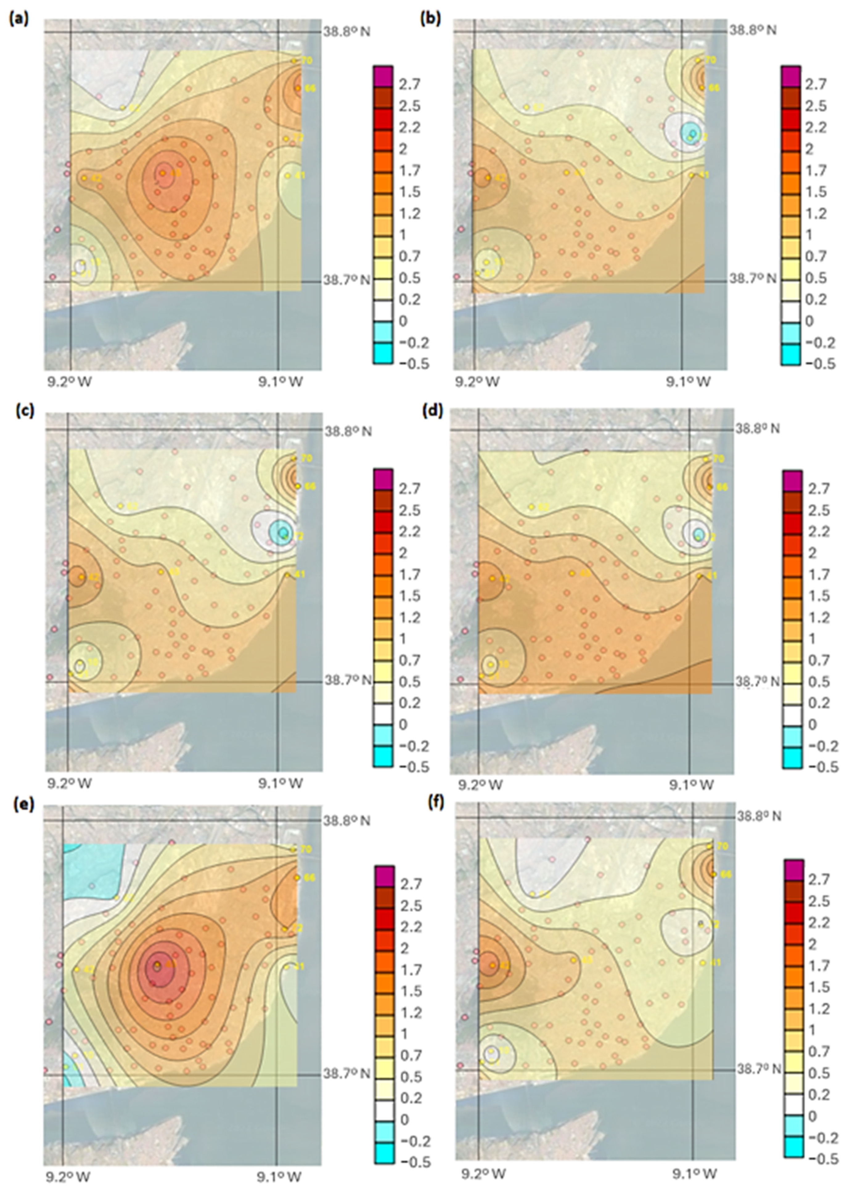
A markedly higher intensity of the UHI effect is evident in sensors positioned in areas categorized as high-density, particularly those identified as within the continuous built fabric class according to COS2018. This is especially pronounced in regions with predominantly vertical structures, which correspond to higher indexes of aerodynamic roughness, building compactness, and liquid construction. These zones tend to exhibit high H/W ratios due to their dense street networks, limited ventilation, and the reduced visible portion of the sky, resulting in a lower sky view factor. Sensor 45 (Rua Frei Carlos) exemplifies this, recording the highest daytime temperatures within the sample and the second-highest daily averages. Similarly, sensor 66 (Rua Ilha dos Amores) exhibits the highest overall average temperatures, ranking second in the roughness index, and is situated in a area predominantly of the vertical continuous built fabric class. This confirms the trend of increased aerodynamic friction and reduced ventilation at an altitude of 5 m, and it is sheltered from prevailing winds compared to the Lisbon Airport reference station (LPPT). Both sensors 45 and 66 are in areas of high urban density.

In contrast, the sensors registering the lowest UHI intensity are 10 (Rua Sá Nogueira), 41 (Jardim do Braço de Prata), 62 (Estrada do Paço do Lumiar), and 70 (Rua Chen He). These sensors are located in low-density urban areas and feature some of the lowest roughness indexes within the sample. Specifically, sensor 10 has the fourth-lowest roughness index, sensor 41 the second lowest, sensor 62 the third lowest, and sensor 70 holds the lowest roughness index among all of the sensors studied. These sensors also fall into lower compactness categories in terms of their H/W ratios.

Inversely, these sensors exhibit the highest sky view factors, with each maintaining a visible sky portion above 0.930. Additionally, sensor 41 is more exposed to wind from all directions, unobstructed by nearby buildings. This exposure allows it to be more influenced by its proximity to the Tagus River, along with its breezes and evaporative cooling effects. During the study period, the urban freshness island (UFI) effect was observed only at sensor 72 exclusively at night. This effect consistently appeared on clear or slightly cloudy nights (with up to 4/8 cloud coverage). In all instances, the UFI effect coincided with periods of light wind at the Lisbon Airport station (LPPT), located at an altitude of 104 m. During the analysis, periods of reduced wind intensity—coupled with the sensor’s lower altitude of 26 m and situation leeward of the LPPT station in a relatively sheltered area—created favorable conditions for this phenomenon. At night, with a negative energy balance due to the absence of solar radiation and infrared losses, the lack of wind and cloud cover promotes the formation of a radiative thermal inversion layer near the ground. The reduced presence of water vapor, coupled with the absence of mixing, allows for cold air to descend slopes and accumulate in valleys, as observed at sensor 72 (Rua Mário Botas).

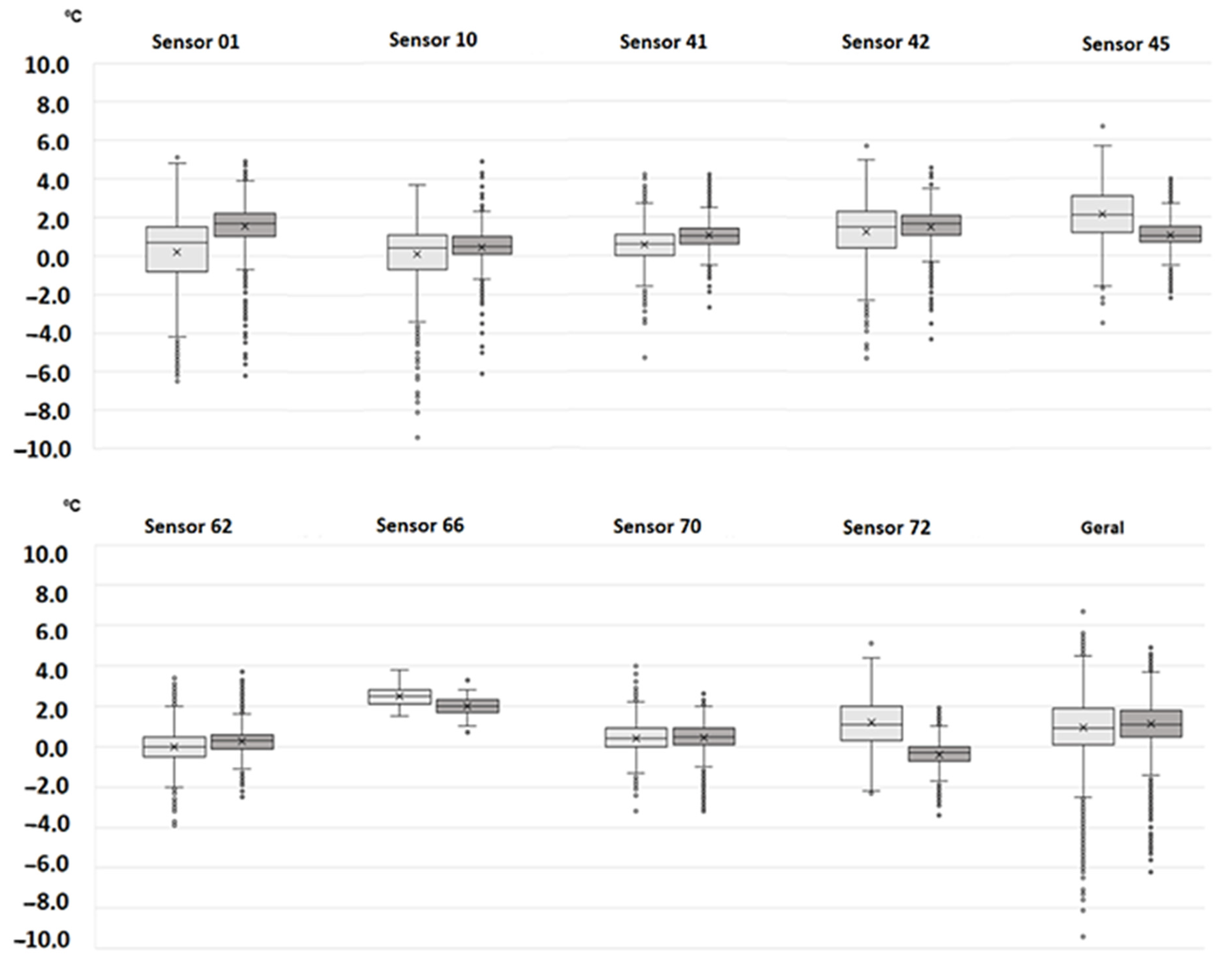
On average, the daily mean UHI effect across all sensors is approximately 0.9 °C, with an average standard deviation of 1.0 °C. Sensor 01 exhibits the highest weighted average standard deviation (1.5 °C), while sensors 70, 62, and 66 show the lowest (0.8 °C, 0.8 °C, and 0.9 °C, respectively), indicating less temperature variability compared to the Lisbon Airport reference station (LPPT). All sensors display higher standard deviations during the day, occasionally nearly double those observed at night, as seen in sensors 01 and 45 (Figure 9, Figures S30 and S31). In conclusion, Rua Frei Carlos, Entrecampos (sensor 45) experiences a pronounced daytime UHI effect, contrasting with other sensors which recorded UHI effects that were more intense at night, such as Travessa Francisco Rezende, Benfica (sensor 42). Rua Ilha dos Amores, Parque das Nações (sensor 66) consistently exhibits a strong UHI effect both in the daytime and at night, maintaining levels close to 2 °C (Figure 7).

Figure 7. UHI intensity maps (°C) at all analyzed points, for the daytime (10:00 to 18:00 UTC) (a), nighttime (20:00 to 06:00 UTC) (b), at 00:00 UTC (c), at 06:00 UTC (d), at 12:00 UTC (e), and at 18:00 UTC (f) (entire network, red dots correspond to unused sensors due to the criteria explained in Section 2.2.3, yellow dots correspond to selected sensors).

Figure 7. UHI intensity maps (°C) at all analyzed points, for the daytime (10:00 to 18:00 UTC) (a), nighttime (20:00 to 06:00 UTC) (b), at 00:00 UTC (c), at 06:00 UTC (d), at 12:00 UTC (e), and at 18:00 UTC (f) (entire network, red dots correspond to unused sensors due to the criteria explained in Section 2.2.3, yellow dots correspond to selected sensors).

3.2.2. Classification of UHI Intensities

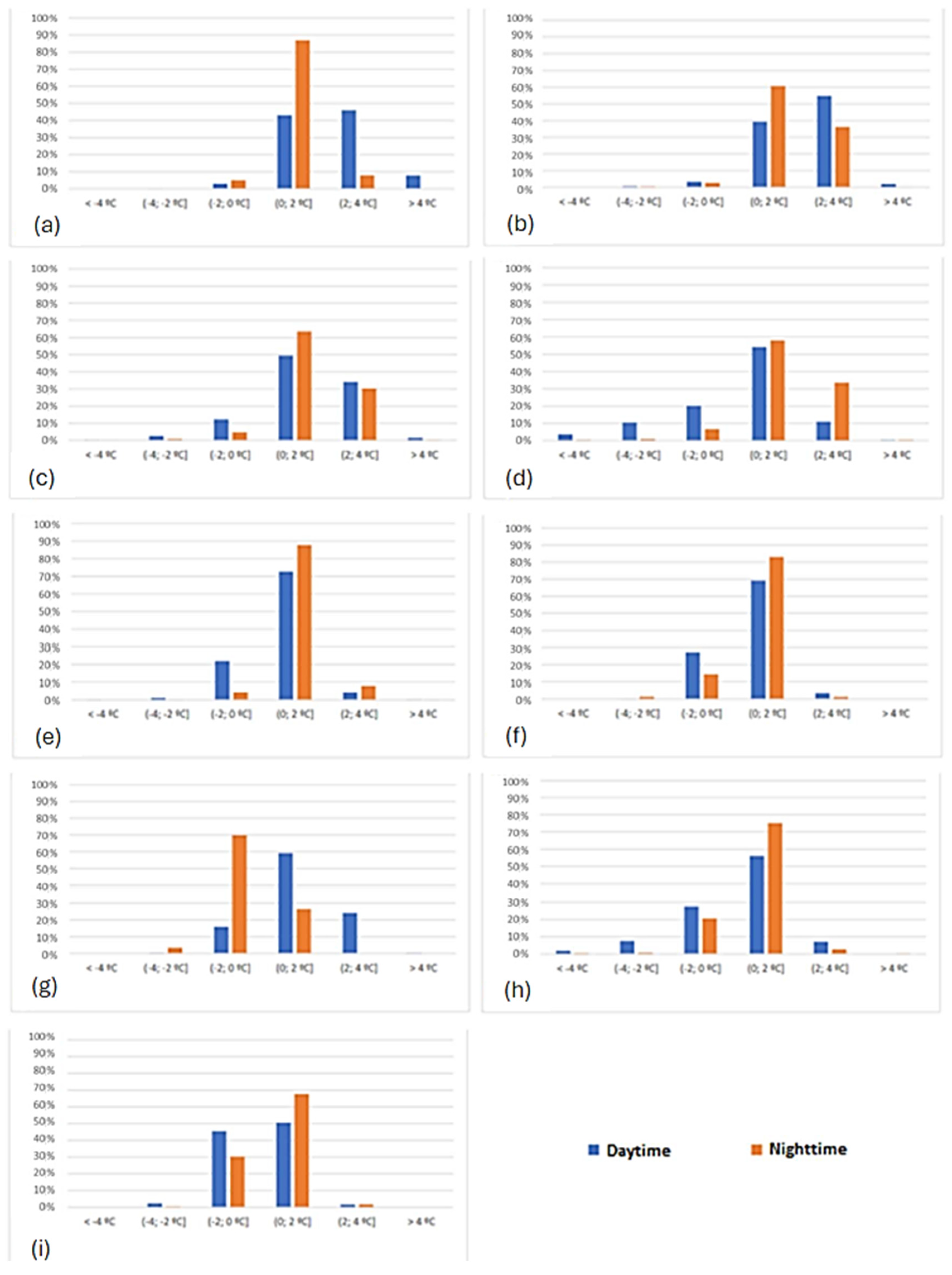
On average, the daily average value of the UHI effect in the overall calculation of the analyzed sensors is around 0.9 °C, with an average standard deviation of 1.0 °C, with sensor 01 having the highest weighted average standard deviation (1.5 °C) and sensors 70, 62, and 66 having the lowest weighted average standard deviation (daily average), with 0.8 °C, 0.8 °C, and 0.9 °C, respectively, which reveals a smaller variation in the temperature values in the latter compared to the reference meteorological station of Lisbon Airport (LPPT). In all of the sensors, there is a higher standard deviation during the day, which is sometimes about twice as high as the standard deviation values verified at night, as is the case in sensors 01 and 45, respectively (Figure 8, Figure 9, Figures S30 and S31).

Figure 8. Daytime and nighttime relative frequencies regarding the local UHI effect for each sensor: (a) sensor 45, (b) sensor 66, (c) sensor 42, (d) sensor 01, (e) sensor 41, (f) sensor 70, (g) sensor 72, (h) sensor 10, and (i) sensor 62.

Figure 8. Daytime and nighttime relative frequencies regarding the local UHI effect for each sensor: (a) sensor 45, (b) sensor 66, (c) sensor 42, (d) sensor 01, (e) sensor 41, (f) sensor 70, (g) sensor 72, (h) sensor 10, and (i) sensor 62.

Figure 9. Temperature deviations referring to the daytime and nighttime periods (light gray and dark gray, respectively), representing Q1, Q2/median, Q3, mean, minimum and maximum values, and outliers.

Figure 9. Temperature deviations referring to the daytime and nighttime periods (light gray and dark gray, respectively), representing Q1, Q2/median, Q3, mean, minimum and maximum values, and outliers.

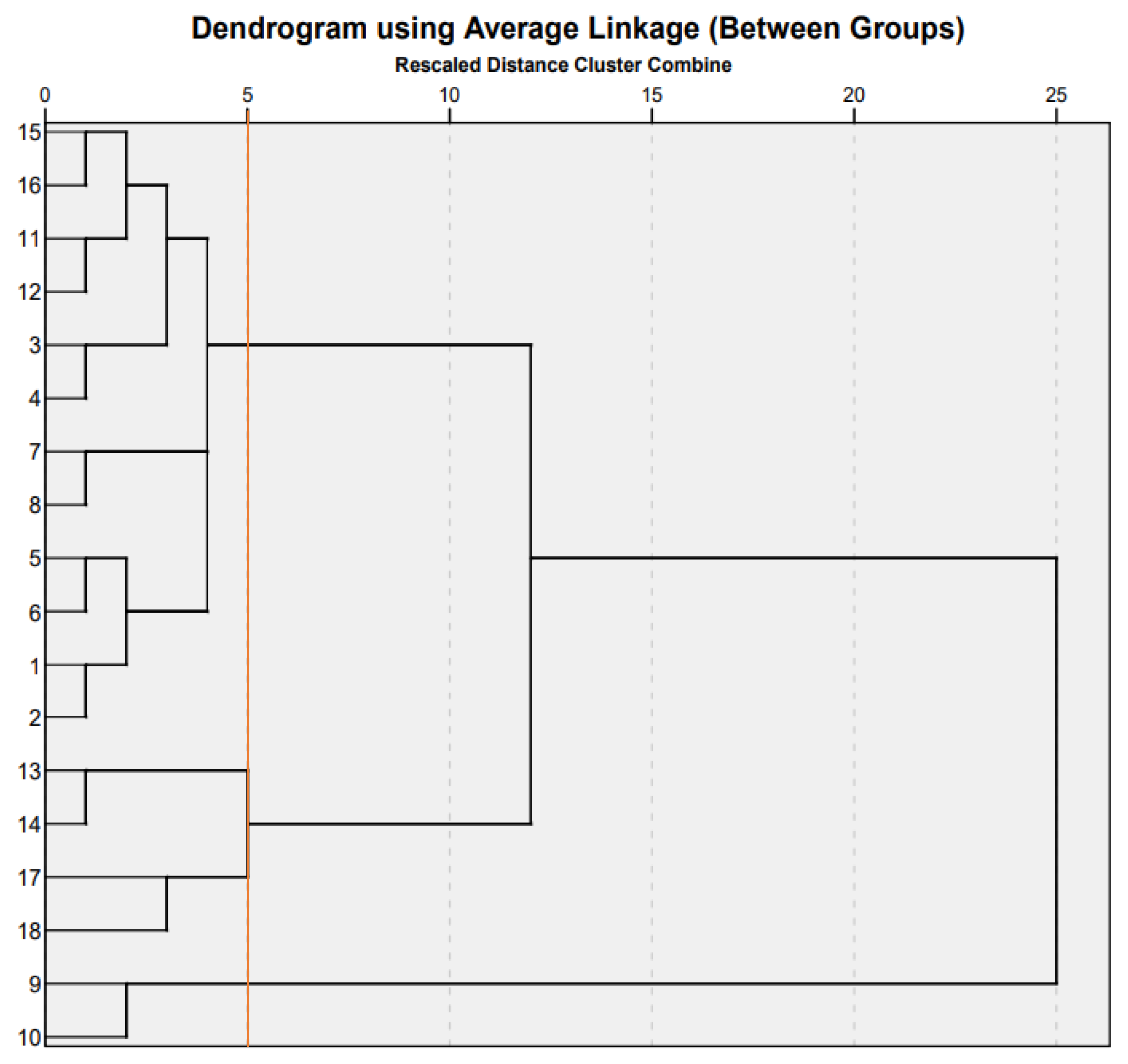
Referring to Figure 10 and

Table 8. The correspondence between sensors and elements in the dendrogram.

	Daily Period	Element in the Dendrogram
Sensor 01	diurnal	01
	nocturnal	02
Sensor 10	diurnal	03
	nocturnal	04
Sensor 41	diurnal	05
	nocturnal	06
Sensor 42	diurnal	07
	nocturnal	08
Sensor 45	diurnal	09
	nocturnal	10
Sensor 62	diurnal	11
	nocturnal	12
Sensor 66	diurnal	13
	nocturnal	14
Sensor 70	diurnal	15
	nocturnal	16
Sensor 72	diurnal	17
	nocturnal	18

, it is possible to conclude that elements 15 and 16 (corresponding to sensor 70 during the daytime and nighttime periods, respectively) are the coldest in the series. They are at the opposite end of elements 9 and 10 (corresponding to sensor 45 during the daytime and nighttime periods, respectively), which have the temperatures with the highest positive deviation in the entire sample in relation to the meteorological station of Lisbon Airport (LPPT), which can be seen in Figures S30 and S31.

Figure 10. Dendrogram of linkage distance between groups (red line corresponds to the cut in the dendrogram done in order to individualize clusters, which is the result of formula 2).

Figure 10. Dendrogram of linkage distance between groups (red line corresponds to the cut in the dendrogram done in order to individualize clusters, which is the result of formula 2).

3.2.3. Land Use and Intensity of UHI

Below, we list the areas by land occupation class (COS2018) and average daily UHI values.

The land occupation class (COS) with the highest temperature values is 1.1.1.1 «Predominantly vertical continuous building fabric (waterproofing greater than 80%)», with an average difference of 1.8 °C in relation to the Lisbon Airport meteorological station (LPPT), followed by COS 1.1.1.2 «Predominantly horizontal continuous building fabric (waterproofing greater than 80%)», with a mean deviation of 1.3 °C. In third place is class 1.7.1.1 «Parks and gardens», with 0.8 °C, and in fourth place is class 1.3.2.2 «Waste and wastewater treatment infrastructure», with 0.5 °C, followed by COS 1.6.5.1 «Other tourist equipment and installations», with 0.4 °C. The land occupancy class (COS2018) with the lowest deviation compared to the reference meteorological station of Lisbon Airport (LPPT) is 1.1.2.2 «Sparse Discontinuous Building Fabric», with only 0.2 °C (

Table 9. Mean UHI effect values in each land use class, in descending order.

Naming Class (COS2018)	Descriptive	Mean Value of the UHI Effect	Sensors That Make Up the Class
1.1.1.1	Predominantly vertical continuous built fabric (waterproofing greater than 80%)	1.8 °C	45, 66
1.1.1.2	Predominantly horizontal continuous built fabric (waterproofing greater than 80%)	1.3 °C	01, 42
1.7.1.1	Parks and gardens	0.8 °C	41
1.3.2.2	Waste and wastewater treatment infrastructure	0.5 °C	70
1.6.5.1	Other tourist equipment and facilities	0.4 °C	10, 72
1.1.2.2	Sparse discontinuous built fabric	0.2 °C	62

).

Furthermore, continuing the spatial analysis of Lisbon based on the density of its areas and following the recommendations of the 2020 report «Identification of Urban Heat Islands and Simulation for Critical Areas in the City of Lisbon», an innovative and more comprehensive analysis was conducted. This analysis incorporates climatopes (Figure S1), following scientific methodologies from reputable publications [35], which combine urban characteristics with local topography and climate.

In the analysis of climatopes (Figure S1), the «High-Density Areas» category recorded the highest temperature values, with an average difference of 1.7 °C compared to the Lisbon Airport meteorological station (LPPT). This was followed by the «Medium Density Areas South of the Aerodynamic Limit» at 1.5 °C. The «Riverfront» climatope ranked third with a difference of 0.6 °C, followed by «Low-Density Areas» at 0.5 °C. The «Shrub and Herbaceous Vegetation and Crops» climatope recorded 0.3 °C, and the «Ventilation Corridors» climatope recorded 0.2 °C, making them the coolest climatopes in the study (

Table 10. Mean UHI effect values in each climatope, in descending order.

Climatope [35]	Mean Value of the UHI Effect	Sensors That Make Up the Class
High-density areas	1.7 °C	45
Areas of medium density south of the aerodynamic limit	1.5 °C	01, 42, 66
Riverfront	0.6 °C	41, 70
Low-density areas	0.5 °C	10, 41, 72
Shrub vegetation, herbs and crops	0.3 °C	62, 70
Ventilation corridors	0.2 °C	62

).

In summary, the areas with the highest UHI effects and the greatest susceptibility to critical thermal stress events are those categorized under land cover classes typically associated with «Vertical Continuous Built Fabric», followed by «Continuous Horizontal Built Fabric», both of which are characterized by soil sealing levels exceeding 80%. It is evident that areas with a higher urban density, characterized by predominantly vertical built fabric, exhibit poorer natural ventilation, higher construction and development rates, lower open space availability, higher aerodynamic roughness, greater compactness (H/W ratio), larger volumes, lower sky view factors, and reduced biomass. These factors contribute to these areas being generally warmer and experiencing prolonged UHI effects compared to areas with opposing characteristics.

Conversely, well-planned consolidated areas that prioritize green spaces and effective ventilation, such as those around sensors 41 (Jardim do Braço de Prata) and 62 (Estrada do Paço do Lumiar), display the lowest temperature values across the network of stations used in this study. The case of sensor 70, located in a reclassified area north of Parque das Nações in Beirolas yet not fully consolidated, reflects similar planning principles, resulting in a low UHI effect in that region.

Additionally, it is evident that the area around sensor 41 (Jardim do Braço de Prata) is significantly cooler than the area around sensor 66 (Rua Ilha dos Amores), despite their proximity to the Tagus Estuary. This difference is attributed to the fact that the former is classified as a «Riparian Front» climatope, while the latter is within a «High-Density Area», according to the Lisbon Climatic Orientation Map. Similar observations apply to sensors 62 (Estrada do Paço do Lumiar) and 70 (Rua Chen He), both of which recorded significantly lower temperatures compared to the general sensor data. Sensor 62 is located in an area classified as «Sparse Discontinuous Built Fabric», north of the aerodynamic limit, making it more exposed to prevailing winds (Figures S32 and S33). Additionally, it lies within a «Ventilation Corridors» climatope. Sensor 70, also located north of the aerodynamic limit, falls within the «Shrub, Herbaceous Vegetation and Crops» classification, along with the «Riverfront» slope, which reduces heat accumulation and enhances natural ventilation. All areas south of the aerodynamic limit, as indicated by the climatope map (Figure S1), tend to record higher air temperatures due to lower exposure to prevailing winds, with urban density exacerbating this effect.

3.2.4. Temporal Variation in the UHI Effect

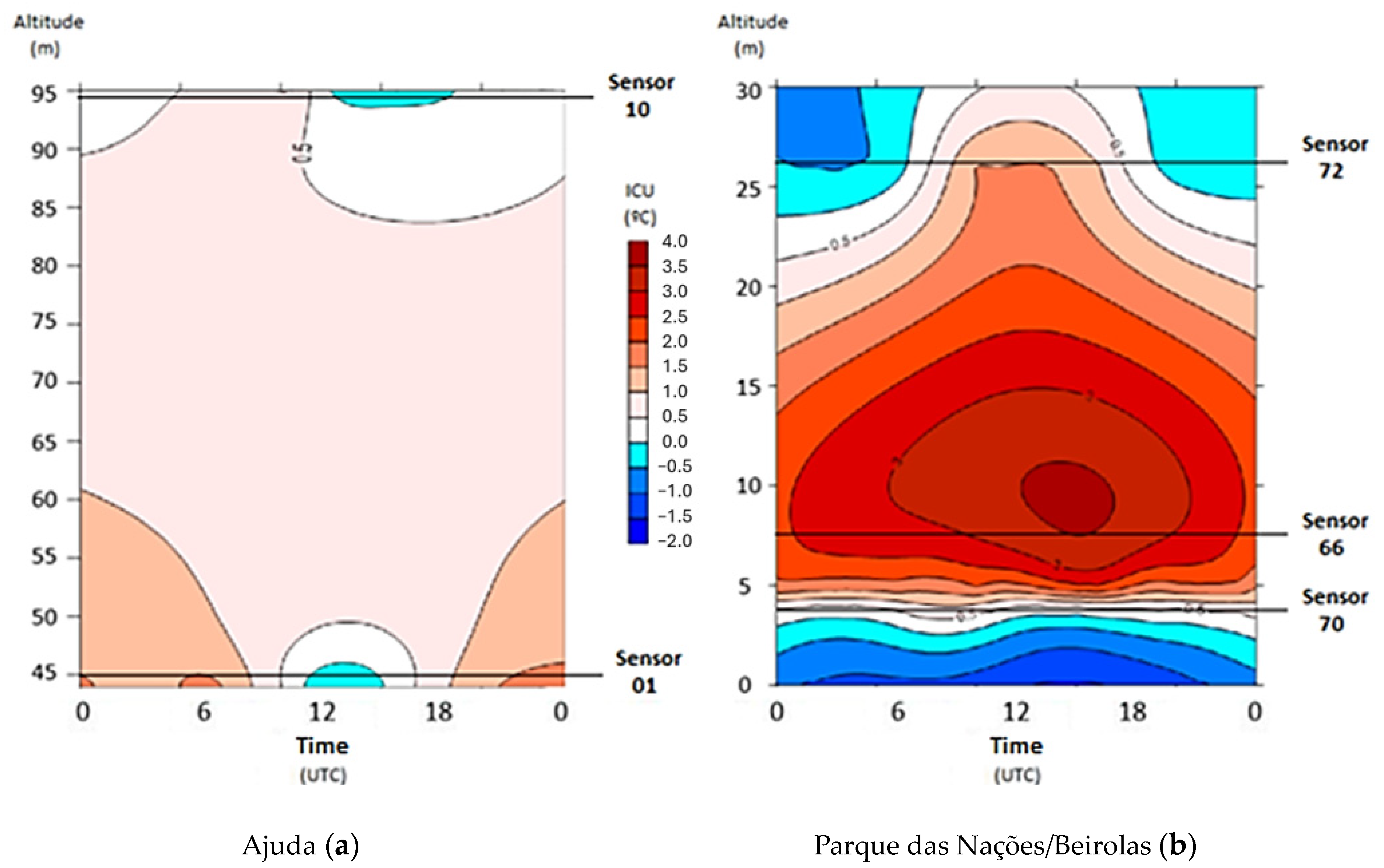
In the case of Figure 11, it is visible that the most intense UHI effect in Ajuda occurs in the sensor located at an altitude of 45 m (sensor 01), especially between 19:00 UTC and 09:00 UTC, with even a slight UFI effect between 11:00 UTC and 15:00 UTC. The same occurs in the highest area of Ajuda, at an altitude of 95 m (sensor 10), although with visibly lower daytime temperatures, as a result of its exposure and lower urban density indexes, aerodynamic roughness, compactness index, volumetry, and higher sky view factor. In the case of the Parque das Nações/Beirolas area, the hottest area is located at an altitude of 6 m, corresponding to sensor 66, which has the highest indexes of compactness, volume, urban density, and aerodynamic roughness, and the lowest sky view factor, added to the fact that it is an area classified as «Predominantly vertical built fabric (waterproofing greater than 80%)» according to COS2018. Sensor 70, located at an altitude of 4 m, is the coolest of the three in this parish, located in an area with an almost total absence of buildings and plenty of green areas. Sensor 72 is located at an altitude of 27 m, in an area with a higher urban density and roughness index compared to sensor 70, heating up visibly but only during the daytime (Figure 11). These thermoisopleth maps contribute to our understanding of the vertical distribution of air temperature patterns and are evidence of the relation between the urban indexes and the thermal patterns, in line with most of the known studies in the field.

Figure 11. Three-point thermoisopleths for visualization of spatial proximity thermal contrasts, referring to the lower urban atmosphere (3 m above ground level) in the areas of Ajuda (a) and Parque das Nações/Beirolas (b). Representation based on mean values of the entire observation period.

Figure 11. Three-point thermoisopleths for visualization of spatial proximity thermal contrasts, referring to the lower urban atmosphere (3 m above ground level) in the areas of Ajuda (a) and Parque das Nações/Beirolas (b). Representation based on mean values of the entire observation period.

Figure 12 and Figure 13 make it possible to identify the behavior of the UHI intensity throughout the day in the various sensors, highlighting the topography of the selected axes (Ajuda and Parque das Nações/Beirolas) in cross-sections, following the northeast–southwest and north–south directions, respectively, from left to right. All these sensors are located on very heterogeneous areas (Figure S1, Tables S19–S29) in terms of land use, climatopes, net construction index, implantation index, open space index, number of floors in the sensor area, aerodynamic roughness index, volumetry index, compactness index (H/W), urban density classes, biomass (maximum annual value), and sky view factor (SVF), which is the reason why some of them exhibit different temperature patterns despite being located relatively close to each other within the same parish.

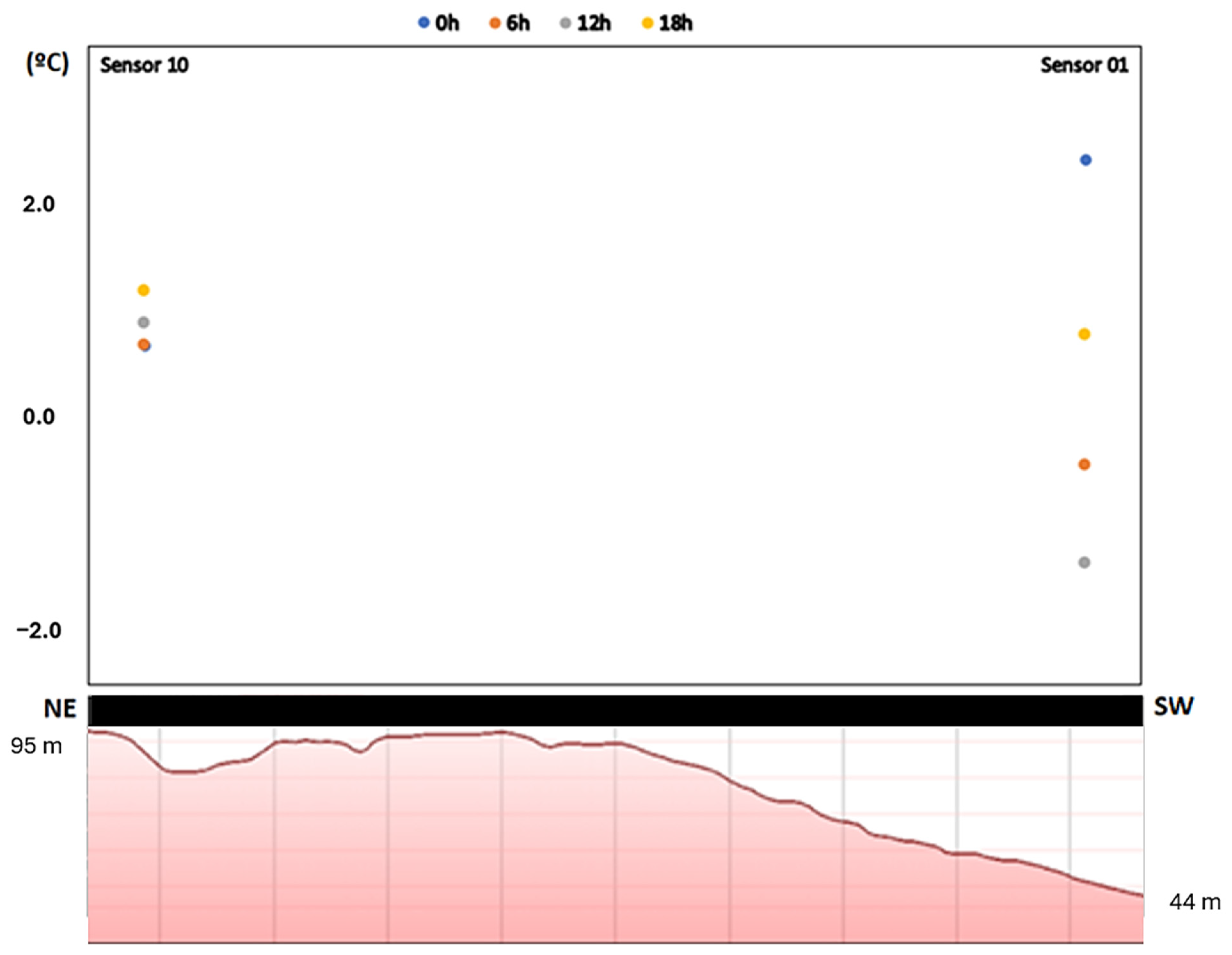
Figure 12. Northeast–southwest axis representing the location of sensors 01 and 10 and the surrounding topography (Ajuda). Representation of the UHI values in the referred locations at 00:00 UTC, 06:00 UTC, 12:00 UTC, and 18:00 UTC on 10 July 2021.

Figure 12. Northeast–southwest axis representing the location of sensors 01 and 10 and the surrounding topography (Ajuda). Representation of the UHI values in the referred locations at 00:00 UTC, 06:00 UTC, 12:00 UTC, and 18:00 UTC on 10 July 2021.

The urban climate literature has highlighted the remarkable prominence of the nighttime UHI phenomenon. At night, UHI effects become more evident due to the greater thermal inertia of the materials used in urban areas [24,25]. These results in particular validate this perspective: areas with a greater urban density, with permanently vertical built fabric, worse natural ventilation conditions, higher construction and deployment rates, lower open space rates, higher aerodynamic roughness rates, higher compactness values (H/W), and higher volumes, as well as a lower sky view factor and biomass values, are generally warmer. These areas also have a greater tendency for thermal inertia, prolonging the UHI effect until later compared to areas with the opposite characteristics. Land use has a great impact on the UHI effect, with continuous, vertical building areas showing the greatest deviations to the reference.

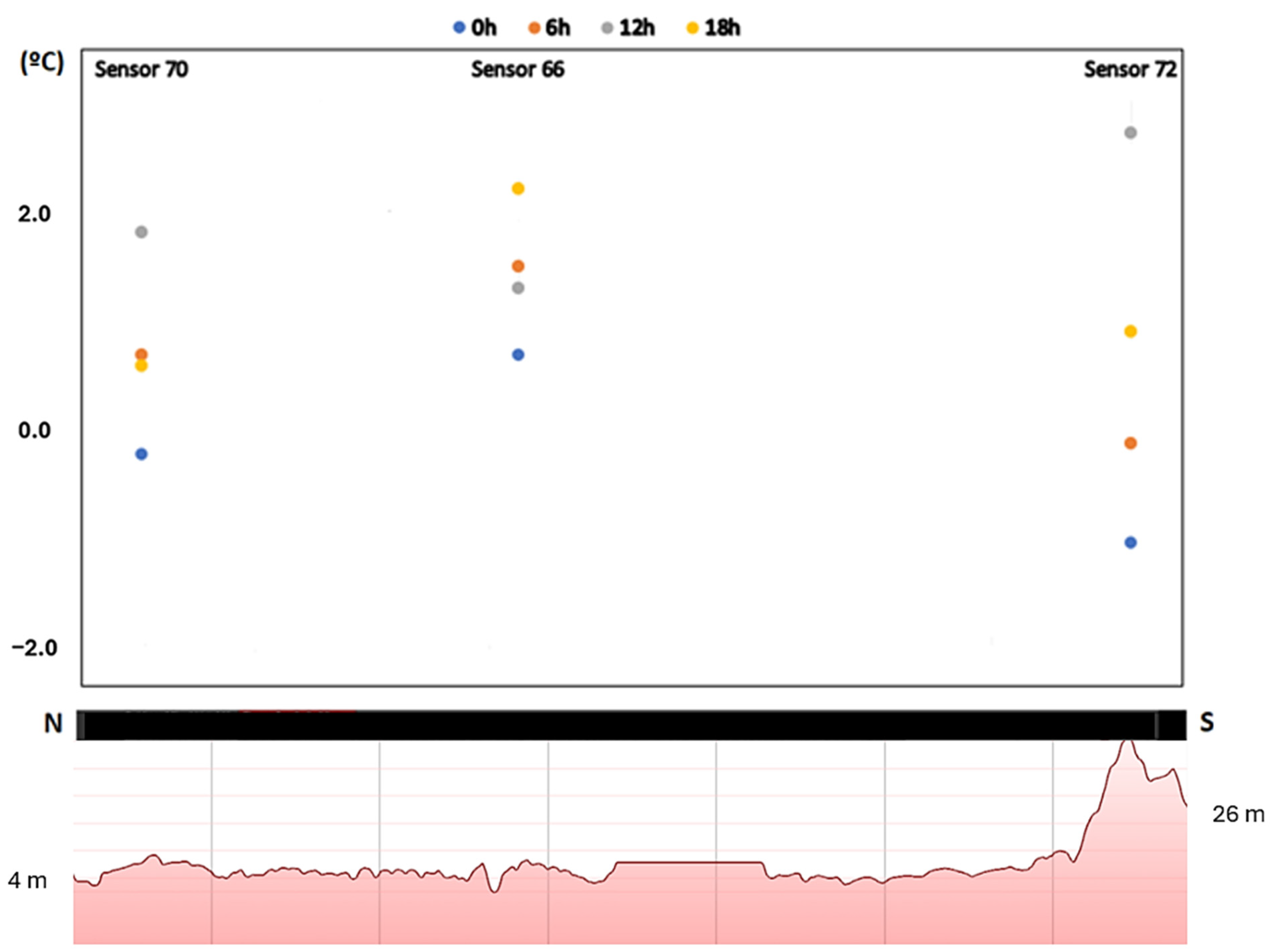
Figure 13. North–south axis representing the location of sensors 66, 70, and 72 and the surrounding topography (Parque das Nações/Beirolas). Representation of the UHI values in the referred locations at 00:00 UTC, 06:00 UTC, 12:00 UTC, and 18:00 UTC on 10 July 2021.

Figure 13. North–south axis representing the location of sensors 66, 70, and 72 and the surrounding topography (Parque das Nações/Beirolas). Representation of the UHI values in the referred locations at 00:00 UTC, 06:00 UTC, 12:00 UTC, and 18:00 UTC on 10 July 2021.

The Case of 10 July 2021: Axis Cross-Section and UHI Effect Per Synoptic Hour (Ajuda)

In the case of Ajuda, a greater range of temperature differentials (the UHI effect and/or the UFI effect) in areas with a lower urban density stands out (in the case of sensor 01 vs. sensor 10). Sensor 01, which is in a lower and denser area, recorded temperatures in the late afternoon (around 6 pm) and at night (around midnight) that were much higher than those recorded at Lisbon Airport (LPPT), surpassing the values of sensor 10, which was installed in an area with the following characteristics:

• The highest altitude;
• The lowest number of floors in the sensor area;
• A lower roughness index (Z0);
• A lower volumetry index;
• The lowest H/W index;
• A greater sky view factor;
• A lower urban density;
• The highest maximum biomass value (between winter and summer).

The Case of 10 July 2021: Axis Cross-Section and UHI Effect Per Synoptic Hour (Parque Das Nações/Beirolas)

In the case of Parque das Nações/Beirolas, the greatest amplitude in temperature differentials in relation to the regional station, Lisbon Airport (LPPT), is recorded by sensor 72, located on the southern edge of Jardim do Cabeço das Rolas, in an area exposed to the southeast that experiences a lot of daytime heating, but with colder nights than the other sensors, with incidents of the UFI effect. The second highest amplitude of the temperature differential compared to the reference station is recorded by sensor 70, one of the least hot in the series addressed, located in an area of low urban density, with a high level of ventilation and a high sky view factor.

Sensor 66, which is in a very low (5 m altitude) and denser area, recorded temperatures in the late afternoon (6 pm values) and at dawn (6 am values) that were much higher than those recorded at Lisbon Airport (LPPT), surpassing the values of sensors 70 and 72, installed in areas with the following characteristics:

• A higher altitude (only in the case of sensor 72);
• The lowest number of floors in the sensor area;
• A lower roughness index (Z0) (exclusively in the case of sensor 70);
• A lower volumetry index;
• The lowest H/W index;
• A greater sky view factor;
• A lower urban density.
  • Our aim was to study one specific day in order to show the thermal performance/patterns of each axis. So, to do that, a day in which thermal stress occurred was chosen in the hope that it would provide meaningful results in our analysis. In all the cases analyzed at this point, during the daytime, the less dense areas heat up faster, and the minimum values located in these areas generally are recorded by the sensors between 6 a.m. and 12 a.m. (Figure 12 and Figure 13). This effect is more noticeable in the early hours of the morning and may be associated with the thermal inertia of the materials that make up the city, which is higher in denser areas. This also may be due to the reduced elevation of the sun in the celestial vault during this period, which promotes the extent and duration of areas of shade in places of greater urban density due to the presence of buildings compared to less dense areas. This effect is reduced throughout the day, reaching a point at which there are no thermal differences between the areas towards the afternoon. In fact, the patterns observed on this day were not very different from those of other days, except that of thermal inertia, which was marginally greater.

4. Discussion

It was identified that Lisbon’s climate is significantly influenced by wind patterns shaped by the city’s topography and proximity to the Tagus River [39], including the effects of sea and estuary breezes. Additionally, land use plays a critical role in these dynamics. At the microscale level, vegetation, urban geometry, and albedo were highlighted as the most significant factors impacting climatic conditions. North winds are particularly important, as they help disperse accumulated heat, whether natural or anthropogenic [13], and improve air quality by promoting the dispersion of atmospheric pollutants. Preserving this effect is essential; thus, avoiding the creation of urban canyons that reduce the city’s level of natural ventilation and exposure to the north is crucial. Such developments could hinder pollutant dispersion and degrade air quality due to the increased surface friction caused by the city’s expansion to the north [40,41]. With the ongoing impacts of climate change, urban areas, which are already susceptible to extreme heat, are becoming even more critical hot spots [42,43].

During the day, less dense areas heat up more quickly, and the minimum temperatures recorded by sensors in these areas typically occur between 6 a.m. and 12 p.m. (Figure 12 and Figure 13). A similar pattern is observed in Ajuda’s highest area, at an altitude of 95 m (sensor 10), although with noticeably lower daytime temperatures. This is due to its exposure and lower urban density indices, including lower aerodynamic roughness, compactness, and volumetric indices, as well as its higher sky view factor. In contrast, in the Parque das Nações/Beirolas area, the hottest spot is at an altitude of 6 m, corresponding to sensor 66, which has the highest indices of compactness, volume, urban density, and aerodynamic roughness, and the lowest sky view factor. This effect is most pronounced in the early morning and may be associated with the thermal inertia of materials that make up the city, which is higher in denser areas [22,25,31,32,33,44]. The reduced elevation of the sun during this period promotes shade in densely built areas due to the presence of buildings, prolonging the duration of shade compared to less dense areas. As the day progresses, this effect diminishes, and the thermal differences between dense and less dense areas tend to disappear by the afternoon.

It is evident that the most consolidated and densely built areas are more prone to thermal stress events, as seen with sensors 01 (Calçada da Ajuda), 45 (Rua Frei Carlos), and 66 (Rua Ilha dos Amores). These areas also suffer from poor ventilation compared to other locations, such as those near sensors 10 (Rua Sá Nogueira), 62 (Estrada do Paço do Lumiar), and 70 (Rua Chen He). This observation is supported by the cluster analysis dendrogram (Figure 10), in which sensors 62 (elements 11 and 12 in the dendrogram) and 70 (elements 15 and 16 in the dendrogram) are associated with the lowest temperature values, while sensors 45 (elements 9 and 10 in the dendrogram), 66 (elements 13 and 14 in the dendrogram), and 72 (elements 17 and 18) show the highest values, particularly during the day.

The spatial analysis of Lisbon, based on the density of its areas, aligns with the recommendations of the 2020 report, “Identification of Urban Heat Islands and Simulation for Critical Areas in the City of Lisbon”. This report advocates for a more comprehensive analysis that includes the concept of climatopes, as defined by official methodology [35], which combines urban components with local topography and climate.

In the analysis that includes climatopes, the “High-density areas” climatope shows the highest temperature values, with an average difference of 1.7 °C compared to the Lisbon Airport meteorological station (LPPT). This is followed by “Medium-density areas south of the aerodynamic limit”, with a difference of 1.5 °C. The “Riverfront” climatope ranks third with a difference of 0.6 °C, followed by “Low-density areas” with a difference of 0.5 °C. The “Shrub and herbaceous vegetation and crops” and “Ventilation corridors” climatopes, with differences of 0.3 °C and 0.2 °C, respectively, are the coolest areas in this study, consistent with previous findings [35].

The most important and greatest positive correlations between the variable «average value of temperature deviation» (the dependent variable) and the independent ones are «urban density classes» (0.665), «compactness index» (the H/W index) (0.522), and «roughness index» (Z0) (0.507). In the same matrix, negative correlations between «average value of temperature deviation» (the dependent variable) and the independent variable «maximum biomass» (−0.563) are shown, confirming their contribution to the results of UHI intensities.

In conclusion, areas with higher UHI effect values and a greater likelihood of critical thermal stress events are those classified under land cover classes like “vertical continuous built fabric” and “continuous horizontal built fabric”, both of which have soil sealing levels above 80%. These areas, characterized by a greater urban density, permanent vertical construction, poor natural ventilation, high construction and deployment rates, low open space rates, high aerodynamic roughness values, compactness (H/W), and high volumes, as well as a low sky view factor and biomass, are generally warmer. They also tend to retain heat longer and have a greater tendency for thermal inertia, prolonging the UHI effect until later compared to areas with the opposite characteristics.

Conversely, consolidated areas with proper planning that prioritize green spaces and effective ventilation, such as those around sensors 41 (Jardim do Braço de Prata) and 62 (Estrada do Paço do Lumiar), exhibit the lowest temperature values across the network of stations used in this study. Sensor 70, located in a reclassified area north of Parque das Nações in Beirolas, though not yet fully consolidated, reflects similar planning principles and concerns, resulting in a low UHI effect. Additionally, the area around sensor 41 (Jardim do Braço de Prata) is notably cooler than that of sensor 66 (Rua Ilha dos Amores), despite their proximity to the Tagus Estuary. This difference is attributed to sensor 41 being located in a “Riparian Front” climatope, while sensor 66 is in a “High-Density Area” climatope according to Lisbon’s climatic orientation document [35].

Similarly, sensors 62 (Estrada do Paço do Lumiar) and 70 (Rua Chen He) show significantly lower temperature values compared to the general average of the analyzed sensors. Sensor 62 is in an area classified as “Sparse discontinuous built fabric” and is located north of the aerodynamic limit, making it more exposed to prevailing winds (Figures S32 and S33). This area is also classified as a “Ventilation corridor”. Sensor 70 is also located north of the aerodynamic limit within the “Shrub, herbaceous vegetation, and crops” classification and is situated on a slope classified as “Riverfront”, resulting in less heat accumulation and more effective natural ventilation. All areas south of the aerodynamic limit, regardless of density, tend to record higher air temperatures due to lower levels of exposure to prevailing winds, with urban density exacerbating this effect.

This network of weather stations operated for less than 1 year. It is not possible to make comparisons to previous analyses on the evolution of the city’s urban fabric during the existence of this network. However, we can make conjectures about the thermal performance of the various locations analyzed in the city where different urban planning measures were applied. The temperature variations found between sensors/locations were expected in a heterogeneous field like Lisbon with its contrasting urban indexes and climatopes. Urban parks, trees, and green roofs have been recognized as pivotal by researchers and policymakers, surpassing other influential factors in mitigating urban heat islands in cities with a hot summer Mediterranean climate (Csa) [45] according to the Köppen–Geiger climate classification. The reduction in green spaces is widely known to contribute to increased urban heat, particularly in cities experiencing gradual development characterized by the expansion of built-up areas and a corresponding decline in agricultural lands and green spaces. Global trends in vegetation loss, construction, and industrial activities significantly intensify the urban heat island (UHI) effect. Urban sprawl and industrial growth influence local climate conditions, primarily due to the reduction in green spaces, loss of soil moisture, increased soil erosion, land subsidence, and diminished infiltration rates [46]. Moreover, partial street coverage with trees, such as fraxinus excelsior, has been shown to be a good solution in some cases, providing optimal conditions for thermal comfort [47], although the presence of this tree species is only typical northeast of mainland Portugal, in a colder climate.

4.1. Other Topoclimatic Factors Conditioning the Thermal Patterns Dependent on Other Meteorological Variables

This section aims to list and analyze other meteorological variables that influence the thermal patterns of the analyzed sensors, addressing wind and cloudiness, culminating in the analysis of an identifiable pattern of the urban freshness island (UFI) effect in one of the areas.

4.1.1. Importance of Prevailing Winds and Ventilation

It is shown that the predominant winds during the period of analysis are from the north and northwest octants, with the predominant direction being north–northwest and with a maximum hourly intensity of 22.5 km/h during the daytime period, accompanied by greater dispersion in the direction of the wind, which is more conducive to directional rotations. At night, however, there is less tendency for wind rotation, with a maximum hourly intensity value of 27.2 km/h, also coming from the north–northwest (Figures S32 and S33). The night period sees its average values rise due to the wind speed values recorded at 18:00 UTC (corresponding to the pre-night period, according to respective publications [9]), which reach 32.5 km/h, from the northwest.

The period with the most unstable wind, variable wind rotation, and the lowest average intensity is at 12:00 UTC, with an average maximum hourly value of 19.9 km/h, coming from the north–northwest (Figures S32 and S33). The most exposed areas, especially those with streets that are aligned with the prevailing winds, benefit from having more effective natural ventilation, as is the case with sensors 10, 41, 62, and 70, which recorded temperature drops from 18:00 UTC (the period when the wind intensity increases). The opposite situation occurs for sensors 01 and 42, which recorded an increasing UHI effect throughout the late afternoon that was not affected by this increase in wind on a regional scale (Figure S31).

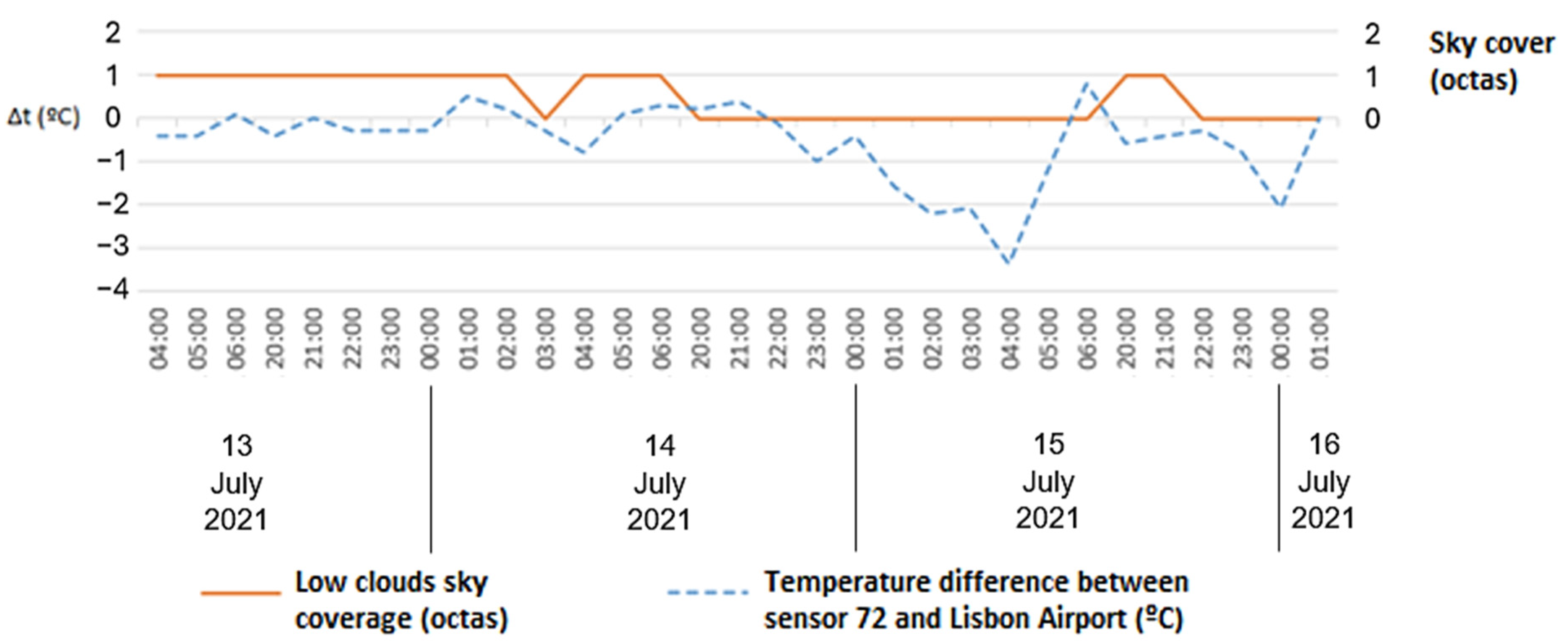
4.1.2. Cloudiness and Urban Freshness Island (UFI)

The case of sensor 72 is particularly illustrative, as it exhibits a pattern of nocturnal cooling, consistently generating an urban freshness island (UFI) effect under the conditions of clear or slightly cloudy skies and light wind. In approximately 90% of the cases, low cloudiness covered no more than 1/8 of the sky, and in 83% of the cases, the average cloudiness remained at or below this threshold. High cloudiness, though less influential in terms of retaining emitted radiation, was analyzed as well, revealing that in 98% of the hourly observations over the approximately seven-month period, cloud cover was nonexistent (Figure S31).

During the analysis period, peaks in the UFI effect at this sensor consistently occurred at night, exclusively on days with clear or slightly cloudy skies (up to 4/8 coverage, Figure S31). This effect was present in 100% of the cases when both of these conditions were met. Notably, this effect often coincided with periods of light wind at the Lisbon Airport meteorological station (LPPT), situated at an altitude of 104 m. Given that this station is quite exposed to wind, any decrease in wind intensity there likely indicates even lower wind speeds at the location of sensor 72, which is at a lower altitude of only 26 m. Furthermore, sensor 72 is positioned leeward of the LPPT station relative to prevailing winds, in a relatively sheltered area compared to the airport. This scenario supports the likelihood of a thermal inversion, a phenomenon that often occurs under these conditions.

Thermal inversions are influenced by radiative exchanges between the atmosphere and the Earth’s surface. During the day, the Earth absorbs short-wavelength radiation (0.15 to 3 μm) from the sun, causing surface warming. At night, the Earth emits longer-wavelength radiation (3 to 100 μm), also known as terrestrial radiation, which is partially absorbed by the atmosphere due to the presence of greenhouse gases like carbon dioxide and water vapor. However, an atmospheric window exists between 8 and 11 μm, allowing for some of this long-wavelength radiation to escape into space, leading to nocturnal radiative cooling, particularly in the absence of cloud cover or fog, which are rich in water vapor and can prevent cooling by enhancing the greenhouse effect. At night, this radiative cooling, combined with the absence of wind and cloud cover, leads to the formation of a near-ground layer of radiative thermal inversion, which is consistent with published literature [20]. The lack of cloud cover and wind facilitates thermal inversions due to reduced water vapor and prevents air mixing, allowing for cold air to drain into valleys, as observed with sensor 72 (Rua Mário Botas). This sensor is located near the southern entrance of Jardim do Cabeço das Rolas and is leeward of the prevailing winds. The garden’s presence may also contribute to sustaining the UFI effect at night at this location, in addition to the physical factors mentioned earlier. The temperature patterns observed at sensor 72 closely align with periods of low cloud cover, showing continuous cooling during clear sky conditions, with temperatures rising again as the cloud cover increases to 1/8 of the sky (Figure 14).

5. Conclusions

This study contributes to the validation of climatopes, aligning with one of the objectives of the Lisbon City Council (CML) and reinforcing the validity of the measures proposed in official literature [35]. The urban heat island (UHI) outputs obtained in this dissertation support the findings of these authors, demonstrating that high-density areas, such as Entrecampos, consistently exhibit higher UHI values compared to low-density areas like Alto da Ajuda, Braço de Prata, Paço do Lumiar, Beirolas, and the southern limit of Parque das Nações. Similarly, areas classified as “bush, herbaceous vegetation and crops” (Paço do Lumiar and Beirolas), “ventilation corridors” (Paço do Lumiar), and “riverside front” (Braço de Prata and Beirolas) also show lower UHI effects. Through our climatope analysis, it is determined that high-density urban areas across Lisbon contribute to an average UHI effect of +1.7 °C, while ventilation corridors have a lower effect of +0.2 °C.

Areas with higher UHI effect values and those more susceptible to critical thermal stress events generally fall into land cover classes such as “vertical continuous built fabric” and “horizontal continuous built fabric”, both of which have soil sealing levels exceeding 80%. These areas, characterized by a high urban density, the predominance of vertical built fabric, poor natural ventilation, higher construction indexes, lower open space indexes, higher aerodynamic roughness, compactness (H/W), and larger building volumetry, as well as a lower sky view factor and biomass values, tend to be warmer. Additionally, these areas exhibit greater thermal inertia, extending the duration of the UHI effect compared to areas with the opposite characteristics. In contrast, consolidated areas with effective urban planning that prioritize green spaces and natural ventilation, such as those around sensors 10 (Rua Sá Nogueira, Ajuda), 62 (Estrada do Paço do Lumiar), and 70 (Rua Chen He, Beirolas), demonstrate the lowest temperature values across the sensor network used in this study. Land use significantly impacts the UHI effect, with continuous, vertical building areas showing the highest average temperature deviations at +1.8 °C, while horizontal building areas show an average of +1.3 °C and sparse, discontinuous built areas show an average UHI effect of +0.2 °C.

We can increase thermal comfort and reduce the effects of the urban heat island through the adoption of planning methods and techniques, including nature-based solutions, as well as low construction rates, aerodynamic roughness values, compactness (H/W) values, and volumes and high levels of open space and a high sky view factor. Plus, the adoption of mitigation and adaptation measures, especially ones based on natural solutions, to climate change and extreme heat events could greatly contribute to maintaining lower levels of thermal stress in these areas. For example, water mirrors, effective shading, afforestation, the increase in green areas irrigated with used rainwater, and the promotion greater evapotranspiration and evaporative cooling are potential solutions in this regard. Examples of these include sensor areas 10 (Rua Sá Nogueira, Ajuda), 62 (Estrada do Paço do Lumiar), and 70 (Rua Chen He, Beirolas), all corresponding to low urban densities, with excellent thermal results, even without the use of all of these measures. These measures may be materialized through territorial management instruments, namely through their implementation in a future Lisbon Master Plan.

Although this study included a higher number of urban indexes than the previous ones, using a total of 11 variables, which were subjected to a principal component analysis, it is important to acknowledge its limitations, particularly the reliance on data from nine sensors and the lack of a broader temporal analysis. The aforementioned nine measurement sites were the only ones meeting installation and data availability standards. Many sites did not have relative humidity data available, and the ones that did recorded very unplausible values, which was the reason why the relative humidity is not considered in this study. Priority was given, within the existing possibilities, to stations with the best installation conditions, with the greatest possible range of data and more constant and reliable records. We also prioritized meteorological stations installed under different conditions within the same parish and used them for comparative purposes in terms of their urban indexes to determine the influence of each of these indexes on the UHI effect. Despite these limitations, the sensors were carefully selected, with a focus on data availability and quality.

Future studies should consider incorporating new sensors with robust data as they become available in order to increase the reproducibility of this study and its methodology. However, our results aligned well with what we initially expected for a great portion of the city and with the expected thermal pattern behavior of each climatope. It would be helpful to expand our understanding of UHI effects across other areas of the city that were not covered in this study and provide a validation of our results on a larger scale.

References

1. Milošević, D.D.; Savić, S.M.; Marković, V.; Arsenović, D.; Šećerov, I. Outdoor human thermal comfort in local climate zones of Novi Sad (Serbia) during heat wave period. Hung. Geogr. Bull. 2016, 65, 129–137. [Google Scholar] [CrossRef]
2. Huang, K.-T.; Yang, S.-R.; Matzarakis, A.; Lin, T.-P. Identifying outdoor thermal risk areas and evaluation of future thermal comfort concerning shading orientation in a traditional settlement. Sci. Total Environ. 2018, 626, 567–580. [Google Scholar] [CrossRef] [PubMed]
3. Huang, C.-H.; Tsai, H.-H.; Chen, H.-C. Influence of weather factors on thermal comfort in subtropical urban environments. Sustainability 2020, 12, 2001. [Google Scholar] [CrossRef]
4. Kim, Y.J.; Brown, R.D. A multilevel approach for assessing the effects of microclimatic urban design on pedestrian thermal comfort: The High Line in New York. Build. Environ. 2021, 205, 108244. [Google Scholar] [CrossRef]
5. Alcoforado, M.; Lopes, A.; Andrade, H.; Vasconcelos, J. Orientações Climáticas Para o Ordenamento em Lisboa; Universidade de Lisboa: Lisboa, Portugal, 2005; pp. 60–61. Available online: https://www.researchgate.net/publication/262567483_Orientacoes_Climaticas_para_o_Ordenamento_em_Lisboa (accessed on 15 August 2022).
6. Alcoforado, M.; Andrade, H. Clima e Saúde na cidade. Implicações para o ordenamento. In A Cidade e a Saúde; Santana, P., Ed.; Edições Almedina, SA, Lisboa: Lisboa, Portugal, 2007; pp. 99–118. [Google Scholar]
7. Andrade, H. O clima urbano-natureza, escalas de análise e aplicabilidade. Finisterra 2005, 40. [Google Scholar] [CrossRef]
8. Alcoforado, M.-J.; Andrade, H.; Lopes, A.; Vasconcelos, J. Application of climatic guidelines to urban planning. Landsc. Urban Plan. 2009, 90, 56–65. [Google Scholar] [CrossRef]
9. Lopes, A.; Alves, E.; Alcoforado, M.J.; Machete, R. Lisbon Urban Heat Island Updated: New Highlights about the Relationships between Thermal Patterns and Wind Regimes. Adv. Meteorol. 2013, 2013, 487695. [Google Scholar] [CrossRef]
10. Alcoforado, M.J.; Andrade, H.; Lopes, A. Urban Climate Maps in Lisbon, Portugal. In Urban Climatic Map—An Information Tool for Sustainable Urban Planning (Chinese Version); Chao, R., Ng, E., Eds.; The China Architecture & Building Press: Beijing, China, 2012; pp. 95–110. ISBN 9787112136377. [Google Scholar]
11. Soares, P.M.M.; Cardoso, R.M.; Semedo, Á.; Chinita, M.J.; Ranjha, R. Climatology of the Iberia coastal low-level wind jet: Weather research forecasting model high-resolution results. Tellus A Dyn. Meteorol. Oceanogr. 2014, 66, 22377. [Google Scholar] [CrossRef]
12. Lima, D.C.; Bento, V.A.; Lemos, G.; Nogueira, M.; Soares, P.M. A multi-variable constrained ensemble of regional climate projections under multi-scenarios for Portugal—Part II: Sectoral climate indices. Clim. Serv. 2023, 30, 100377. [Google Scholar] [CrossRef]
13. Lopes, A.; Saraiva, J.; Alcoforado, M. Urban boundary layer wind speed reduction in summer due to urban growth and environmental consequences in Lisbon. Environ. Model. Softw. 2011, 26, 241–243. [Google Scholar] [CrossRef]
14. Alcoforado, M.-J.; Andrade, H. Nocturnal urban heat island in Lisbon (Portugal): Main features and modelling attempts. Theor. Appl. Clim. 2006, 84, 151–159. [Google Scholar] [CrossRef]
15. Reis, C. A Eficiência Térmica no Potencial de Arrefecimento de dois Espaços Verdes em Lisboa. Master’s Thesis, IGOT, Universidade de Lisboa, Lisboa, Portugal, 2018. [Google Scholar]
16. Greater London Authority. London’s Urban Heat Island: A Summary for Decision Makers; Greater London Authority: London, UK, 2006.
17. Rutledge, K.; Ramroop, T.; Boudreau, D.; McDaniel, M.; Teng, S.; Sprout, E.; Costa, H. Urban Heat Island. 2011. Available online: https://www.nationalgeographic.org/encyclopedia/urban-heat-island/ (accessed on 25 July 2022).
18. Sabnis, G. Green Building with Concrete: Sustainable Design and Construction; CRC Press: Boca Raton, FL, USA, 2015. [Google Scholar]
19. Oke, T.R. The energetic basis of the urban heat island. Q. J. R. Meteorol. Soc. 1982, 108, 1–24. [Google Scholar] [CrossRef]
20. Roth, M.; Oke, T.R. Turbulent transfer relationships over an urban surface. I. Spectral characteristics. Q. J. R. Meteorol. Soc. 1993, 119, 1071–1104. [Google Scholar]
21. Garratt, J. Boundary layer climates. Earth-Sci. Rev. 1987, 27, 265. [Google Scholar] [CrossRef]
22. Alverson, K.; Bailey, W.G.; Oke, T.R.; Rouse, W.R. The surface climates of Canada. Arct. Alp. Res. 1997, 30, 418. [Google Scholar] [CrossRef]
23. Voogt, J.A.; Oke, T.R. Thermal remote sensing of urban climates. Remote Sens. Environ. 2003, 86, 370–384. [Google Scholar] [CrossRef]
24. Oke, T.; Mills, G.; Christen, A.; Voogt, J. Urban Climate; Cambridge University Press: Cambridge, UK, 2017; pp. 156–158. [Google Scholar]
25. Oliveira, A.; Lopes, A.; Correia, E.; Niza, S.; Soares, A. Heatwaves and Summer Urban Heat Islands: A Daily Cycle Approach to Unveil the Urban Thermal Signal Changes in Lisbon, Portugal. Atmosphere 2021, 12, 292. [Google Scholar] [CrossRef]
26. Lopes, A. O sobreaquecimento das cidades. Causas e medidas para a mitigação da ilha de calor de Lisboa. Territorium 2008, 15, 39–52. [Google Scholar] [CrossRef]
27. Andrade, H.; Alcoforado, M.-J. Microclimatic variation of thermal comfort in a district of Lisbon (Telheiras) at night. Theor. Appl. Clim. 2007, 92, 225–237. [Google Scholar] [CrossRef]
28. Arnfield, A. Two decades of urban climate research: A review of turbulence, exchanges of energy and water, and the urban heat island. Int. J. Climatol. A J. R. Meteorol. Soc. 2003, 23, 1–26. [Google Scholar] [CrossRef]
29. Oliveira, S.; Andrade, H. An initial assessment of the bioclimatic comfort in an outdoor public space in Lisbon. Int. J. Biometeorol. 2007, 52, 69–84. [Google Scholar] [CrossRef]
30. Stewart, I.D.; Oke, T.R. Local Climate Zones for Urban Temperature Studies. Bull. Am. Meteorol. Soc. 2012, 93, 1879–1900. [Google Scholar] [CrossRef]
31. Geletič, J.; Lehnert, M.; Savić, S.; Milošević, D. Modelled spatiotemporal variability of outdoor thermal comfort in local climate zones of the city of Brno, Czech Republic. Sci. Total Environ. 2018, 624, 385–395. [Google Scholar] [CrossRef] [PubMed]
32. Lau, K.K.-L.; Shi, Y.; Ng, E.Y.-Y. Dynamic response of pedestrian thermal comfort under outdoor transient conditions. Int. J. Biometeorol. 2019, 63, 979–989. [Google Scholar] [CrossRef] [PubMed]
33. Lau, K.K.-L.; Tan, Z.; Morakinyo, T.E.; Ren, C. Outdoor Thermal Comfort in Urban Environment: Assessments and Applications in Urban Planning and Design, 1st ed.; Springer: Singapore, 2022. [Google Scholar] [CrossRef]
34. Unger, J.; Skarbit, N.; Gál, T. Evaluation of outdoor human thermal sensation of local climate zones based on long-term database. Int. J. Biometeorol. 2018, 62, 183–193. [Google Scholar] [CrossRef] [PubMed]
35. Lopes, A.; Vasconcelos, J.; Correia, E. Identificação das ilhas de calor urbano e simulação para as áreas críticas da cidade de Lisboa. In Fase 3—Relatório Final de Cenarização e Mapeamento de Medidas de Mitigação das Ilhas de Calor Urbano; Câmara Municipal de Lisboa: Lisbon, Portugal, 2020. [Google Scholar]
36. Oke, T. Initial Guidance to Obtain Representative Meteorological Observations at Urban Sites; WMO/TD-No. 1250; World Meteorological Organization: Vancouver, BC, Canada, 2004; p. 51. [Google Scholar]
37. Marôco, J. Análise Estatística—Com Utilização do SPSS, 3rd ed.; Edições Sílabo: Lisboa, Portugal, 2007. [Google Scholar]
38. Chang, J.; Shoshany, M. Mediterranean shrublands biomass estimation using Sentinel-1 and Sentinel-2. In Proceedings of the 2016 IEEE International Geoscience and Remote Sensing Symposium (IGARSS), Beijing, China, 10–15 July 2016; 2016; pp. 5300–5303. [Google Scholar] [CrossRef]
39. Andrade, H. Bioclima Humano e Temperatura do ar em Lisboa; Universidade de Lisboa: Lisbon, Portugal, 2003. [Google Scholar]
40. Lopes, A. Modificações no Clima de Lisboa Como Consequência do Crescimento Urbano. Vento, ilha de calor de Superfície e Balanço Energético. In Tese de Doutoramento em Geografia Física Apresentada à Faculdade de Letras da Universidade de Lisboa; Univerisdade de Lisboa: Lisboa, Portugal, 2003; 354p. [Google Scholar]
41. Alcoforado, M.J.; Lopes, A.; Andrade, H. Urban Climatic Map Studies in Portugal: Lisbon. In The Urban Climatic Map for Sustainable Urban Living; Ng, E., Ren, C., Eds.; Routledge: London, UK, 2015; Chapter 16. [Google Scholar]
42. Foshag, K.; Aeschbach, N.; Höfle, B.; Winkler, R.; Siegmund, A.; Aeschbach, W. Viability of public spaces in cities under increasing heat: A transdisciplinary approach. Sustain. Cities Soc. 2020, 59, 102215. [Google Scholar] [CrossRef]
43. Reis, C.; Lopes, A.; Correia, E.; Fragoso, M. Local weather types by thermal periods: Deepening the knowledge about Lisbon’s urban climate. Atmosphere 2020, 11, 840. [Google Scholar] [CrossRef]
44. Oliveira, S.; Vaz, T.; Andrade, H. Perception of termal comfort by users of urban green areas in Lisbon. Finisterra—Rev. Port. De Geogr. 2014, XLIX, 113–131. [Google Scholar]
45. Karimi, A.; Mohammad, P.; García-Martínez, A.; Moreno-Rangel, D.; Gachkar, D.; Gachkar, S. New developments and future challenges in reducing and controlling heat island effect in urban areas. Environ. Dev. Sustain. 2023, 25, 10485–10531. [Google Scholar] [CrossRef]
46. Halder, B.; Karimi, A.; Mohammad, P.; Bandyopadhyay, J.; Brown, R.D.; Yaseen, Z.M. Investigating the relationship between land alteration and the urban heat island of Seville city using multi-temporal Landsat data. Theor. Appl. Clim. 2022, 150, 613–635. [Google Scholar] [CrossRef]
47. Mohammad, P.; Aghlmand, S.; Fadaei, A.; Gachkar, S.; Gachkar, D.; Karimi, A. Evaluating the role of the albedo of material and vegetation scenarios along the urban street canyon for improving pedestrian thermal comfort outdoors. Urban Clim. 2021, 40, 100993. [Google Scholar] [CrossRef]
Figure 1. Methodological scheme of data acquisition and treatment.
Atmosphere 15 01177 g001
Figure 2. Location of the temperature sensors of the Lisbon Aberta network from CML in the municipality of Lisbon (entire network, red dots correspond to unused sensors due to the criteria explained in Section 2.2.3, yellow dots correspond to selected sensors).
Atmosphere 15 01177 g002
Figure 3. Time period used for data analysis in each sensor of CML’s Lisboa Aberta network.
Atmosphere 15 01177 g003
Figure 14. Relation between the presence of low cloudiness (in octas of covered sky) and the thermal difference between sensor 72 and the Lisbon Airport meteorological station (LPPT) at night between 13 July 2021 and 16 July 2021.
Atmosphere 15 01177 g014