Article

The Spatio-Temporal Distribution Characteristics of Carbon Dioxide Derived from the Trajectory Mapping of Ground Observation Network Data in Shanxi Province, One of China’s Largest Emission Regions

1
Shanxi Institute of Meteorological Science, Taiyuan 030002, China
2
Shanxi Branch of Monitoring and Assessment Center for GHGs & Carbon Neutrality, China Meteorological Administration, Taiyuan 030002, China
3
Wutaishan Cloud Physics Field Experiment Base, China Meteorological Administration, Xinzhou 035514, China
4
Beijing Mailbox 5111, Beijing 100094, China
5
Shanxi Provincial Weather Modification Center, Taiyuan 030032, China
*
Authors to whom correspondence should be addressed.
Atmosphere 2024, 15(1), 98; https://doi.org/10.3390/atmos15010098
Submission received: 10 December 2023 / Revised: 2 January 2024 / Accepted: 5 January 2024 / Published: 12 January 2024
(This article belongs to the Section Atmospheric Techniques, Instruments, and Modeling)

Abstract

:
In this study, the trajectory mapping domain-filling technology, which can provide more reliable statistical estimates of long-lived gas concentrations in a broader geographical area based on limited station data, is used to map the CO2 concentration data of six ground observation stations to the entire Shanxi Province. The technology combines a dynamical model of the atmosphere with trace gas observations, combining forward and backward trajectories to greatly expand the information on long-lived CO2 gas concentrations over a trajectory path. The mapped results show good agreement with the observation results, which reveals the generalizability of the trajectory mapping domain-filling technology. The results show that the spatio-temporal distribution characteristics of CO2 concentration in the entire Shanxi region is significant: during the five years, the provincial average CO2 concentration exhibits an overall increasing trend. The CO2 concentration increases from the north to the south across the province. Influenced by the economic growth rate and COVID-19, there are differences in the annual variation characteristics of the CO2 concentration across the entire province, with the highest year-on-year growth in 2019 and a year-on-year decrease in 2020. The increasing rate of the CO2 concentration in the northern low-value areas is faster than that in the southern high-value areas. Overall, there is a decreasing trend in the CO2 concentration growth from the north to the south in the entire province. There are seasonal differences in the CO2 concentration distribution across the entire province. The CO2 concentration and amplitude are higher in autumn and winter than they are in spring and summer. This study can provide scientific support and methodological reference for the spatio-temporal distribution characteristics analysis of GHGs at the provincial–regional scale, as well as at the national and global scales.

1. Introduction

Carbon dioxide (CO2) is one of the most important greenhouse gases (GHGs) in the Earth’s atmosphere. Since the industrial era, anthropogenic activities have emitted excessive GHGs into the atmosphere, being a dominant cause of climate warming since the 1950s and leading to an increased frequency of extreme weather and climate events. In 2021, the global average CO2 concentration reached 415.7 ± 0.2 ppm, which is the highest in at least two million years [1]. Therefore, it is imperative to take proactive measures to address climate change. The international community has gradually reached a consensus that GHG emission reduction is the most effective way to mitigate global warming. However, the distribution of GHGs worldwide is non-homogeneous and dynamic, and the spatio-temporal variations in GHG concentrations are closely linked to regional emissions [2]. The World Meteorological Organization has organized the Global Atmosphere Watch since the end of the 1960s, comprising more than 200 background stations from over 60 countries. As the world’s leading CO2 emitter country, China completed the construction of the first national observation network by the end of 2021 after nearly 40 years of efforts. This network consists of 60 stations covering key climate regions, including 7 global and regional background stations, as well as 6 national GHG observation stations (Jincheng, Linfen, Taiyuan, Wutaishan, Shuozhou and Datong stations) in Shanxi Province. Among all the provinces in China, Shanxi is a representative province, which is a nationally integrated energy base and a major coal-producing province, and its carbon-intensive energy development model has led to a rapid growth in GHG emissions, ranking first in the country in terms of CO2 emissions for three consecutive years from 2013 to 2015, and still ranking among the top in recent years [3,4]. The study of Shanxi region is representative, which can provide scientific support and methodological reference for the spatio-temporal distribution characteristics analysis of GHGs at the provincial–regional scale, as well as at the national and global scales.
The data from existing online observation stations are sparsely distributed, with limited spatial coverage. Therefore, there are great challenges for the analysis of GHG concentration variations and source/sink characteristics at the regional scale. In the early stages, the studies on long-term CO2 observation in China mainly focused on the variation characteristics of the CO2 concentration at background stations or data filtering [5]. In recent years, scholars at home and abroad have assessed the impacts and role of human activities on the distribution of the atmospheric CO2 concentration in urban areas based on short-term CO2 observations from urban stations, such as Los Angeles [6], Munich [7], Shanghai [8]) and Suzhou [9]. However, due to the limited representativeness of the observation stations, the conclusions drawn from these studies have limited applicability in guiding the formulation of precise regional emission reduction policies.
A spatial domain-filling technique called trajectory mapping can provide more reliable statistical estimates of long-lived gas concentrations in a broader geographical area based on limited station data [10]. Liu et al. [11] have applied this technique to successfully map the distribution of the global tropospheric ozone from 1960 to 2000 and studied its climatological characteristics. Chinese scholars have employed this technique to obtain the spatial-temporal distribution characteristics of regional ozone and the corresponding influencing factors based on the data from the Waliguan global atmospheric background station [12]. Currently, the studies on the regional distribution and patterns of GHGs based on online GHG observations are still deficient. Moreover, research on limited data and information (six national GHG observation stations) being mapped onto the entire province of Shanxi has been less reported.
In this study, based on the high-accuracy online atmospheric CO2 concentration obtained from the six observation stations in Shanxi Province during 2016–2020, along with the global data assimilation system (GDAS) dataset provided by the National Centers for Environmental Prediction (NCEP), we effectively map the CO2 concentration data onto the entire province by using the trajectory-mapped spatial domain-filling technique, and then analyze the spatio-temporal distribution characteristics of CO2 throughout the province. This study aims to reveal the influencing factors of atmospheric CO2 distribution in different areas, thus providing scientific judgments to understand the current regional carbon emissions in Shanxi and formulate an action plan for carbon peaking and carbon neutrality in the region.
The remainder of this paper is organized as follows: The data and methods are provided in Section 2. Section 3 presents the optimal parameterization selection. The results are analyzed in Section 4. Finally, Section 5 gives the conclusions and discussion.

2. Data and Methods

2.1. Ground Observation Network

The six GHG observation stations in Shanxi Province of China, listed from the north to the south, are Datong station, Shuozhou station, Wutaishan station, Taiyuan station, Linfen station and Jincheng station (Figure 1). An overview of the six stations is provided in Table 1.

2.2. Measurements of Atmospheric CO2

The main host of the online observation system of atmospheric CO2 concentration adopts the high-accuracy CO2 analyzer (model: G2301) developed by Picarro Inc., USA, which is based on the wavelength-scanned cavity ring-down spectroscopy technology. The CO2 measurement accuracy is 50 ppb per 5 min, with a maximum drift of 500 ppb per month, and the measurement height is 30 m. The use of standard gases in the observation system, the setup of the 8-port valve, and the method of data quality control refer to Zhang et al. [13]. In this study, the relatively accurate 5 min averages are used as the original data. Then, we exclude the outliers based on station records, including the data obtained during system maintenance periods, such as alcohol replacement in the cold traps and instrument calibration, and the data influenced by human activities, such as a large number of people visiting or garbage burning near the sampling port. After data exclusion, approximately 82.4% of data are retained for statistical analysis.

2.3. Trajectory Calculation and Provincial-Scale CO2 Mapping

Trajectory mapping is a physical-quantity-interpolation-based spatial domain-filling technique that combines atmospheric dynamical models with trace gas observations, and it can address the issue of limited spatial data coverage [14]. This physically based method, in effect, interpolates data based on knowledge of atmospheric transport and offers obvious advantages over typical statistical interpolation methods through its far broader scope of geographic coverage. The technology can thereby provide reliable estimates of measurement accuracy and precision for entire datasets rather than relying upon the extrapolation of results that are achieved through the validation of a small subset of the data through traditional techniques. This study utilizes the hybrid single-particle Lagrangian integrated trajectory (HYSPLIT) model developed by the National Oceanic and Atmospheric Administration. The hourly forward and backward trajectory mapping calculations of online CO2 observations at each station are performed by taking the GDAS data (with a spatial resolution of 1° × 1°) provided by the NCEP (National Centers for Environmental Prediction) reanalysis dataset as input data.
This process allows one online observation to be mapped onto 48–144 new positions along the forward and backward trajectory paths over a period of 24–72 h, thereby greatly spreading out the CO2 information along the trajectory paths and enhancing the density of coverage in our trajectory maps. Then, we plot the CO2 concentration distribution maps of the entire province containing five stations, except one comparative station separately. The results are then cross-validated with the in situ CO2 information from the comparative station [15]). Furthermore, based on some statistical indicators of the two sets of data, such as root mean square error (RMSE), correlation coefficient (R) and relative bias (Bias), the optimal values for the sensitivity parameters are determined [16]). On the basis of the optimal parameter values and the in situ information from the six stations, the CO2 trajectory mapping dataset in Shanxi Province from 2016 to 2020 is obtained. Subsequently, the CO2 distribution characteristics of the entire province are analyzed, and then, the annual variations in the CO2 concentrations of the entire province and 11 cities are calculated.

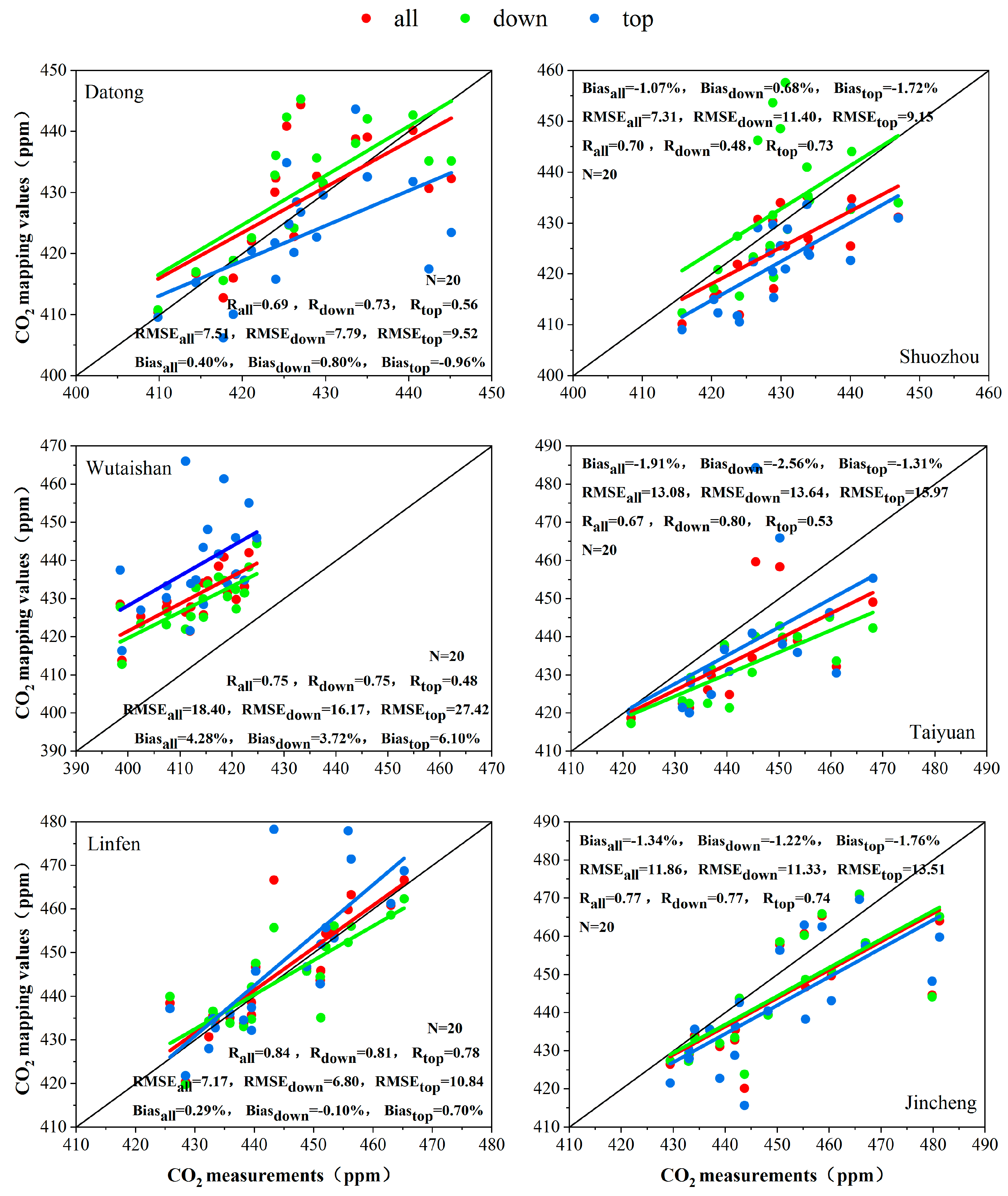
3. Sensitivity Studies

The key to the trajectory mapping technique is to conduct the sensitivity experiments on the two sensitivity parameters, namely, trajectory calculation altitude and trajectory calculation duration [12,16]. A good test of an interpolation model is to examine how it performs in areas where no data are available. In this study, the cross-validation technique is employed to achieve the optimal selection of the two parameters.

3.1. Sensitivity to the Trajectory Calculation Altitude

The trajectory that is run is the initial height set to 300 m above the elevation of each station. Referring to Yan et al. [17], all the trajectories are divided into three groups according to their running heights, namely, all altitudes that are reachable by the trajectory model (the “all” group), altitudes below 2 km that are heavily influenced by human activities (the “down” group), and altitudes above 2 km that are less affected by human activities (the “top” group). For the period of 2016–2020, the hourly online CO2 concentration observations from five stations, excluding one comparative station, are used to perform the forward 24 h and backward 72 h trajectory mapping calculations. The mapped values of the comparative station are extracted from the obtained dataset and then compared with the seasonal averages of the in situ information. The evaluation is conducted by using R, RMSE and Bias [18], as shown in Figure 2.
By comparing Rall, Rdown and Rtop among the six stations, it is evident that the Rdown is the largest at Datong, Wutaishan, Taiyuan and Jincheng stations, which are all significant at the 0.001 level. Although the Rdown of Linfen station is not the largest, it is also significant at the 0.001 level; the Rdown of Shuozhou station is significant at the 0.1 significance level. In terms of the RMSEall, RMSEdown and RMSEtop among the six stations, the minimum RMSEdown is observed at Linfen station, which is only 6.80. Through the comparison of three groups of RMSE at each station, the RMSEdown values at Linfen, Jincheng and Wutaishan stations are the closest to 0, and the RMSEdown values at Taiyuan and Datong stations are also at a low level. A comparison of Biasall, Biasdown and Biastop among the six stations shows that the Biasdown at Linfen station is the closest to 0, with a value of −0.10%. Moreover, the Biasdown values at Linfen, Jincheng, Shuozhou and Wutaishan stations are all closer to 0 than Biasall and Biastop at these four stations. Taking into account the three indicators that characterize the degree of difference between mapped values and in situ information from different perspectives, this study selects an altitude below 2 km as the optimal parameter for the trajectory calculation altitude.

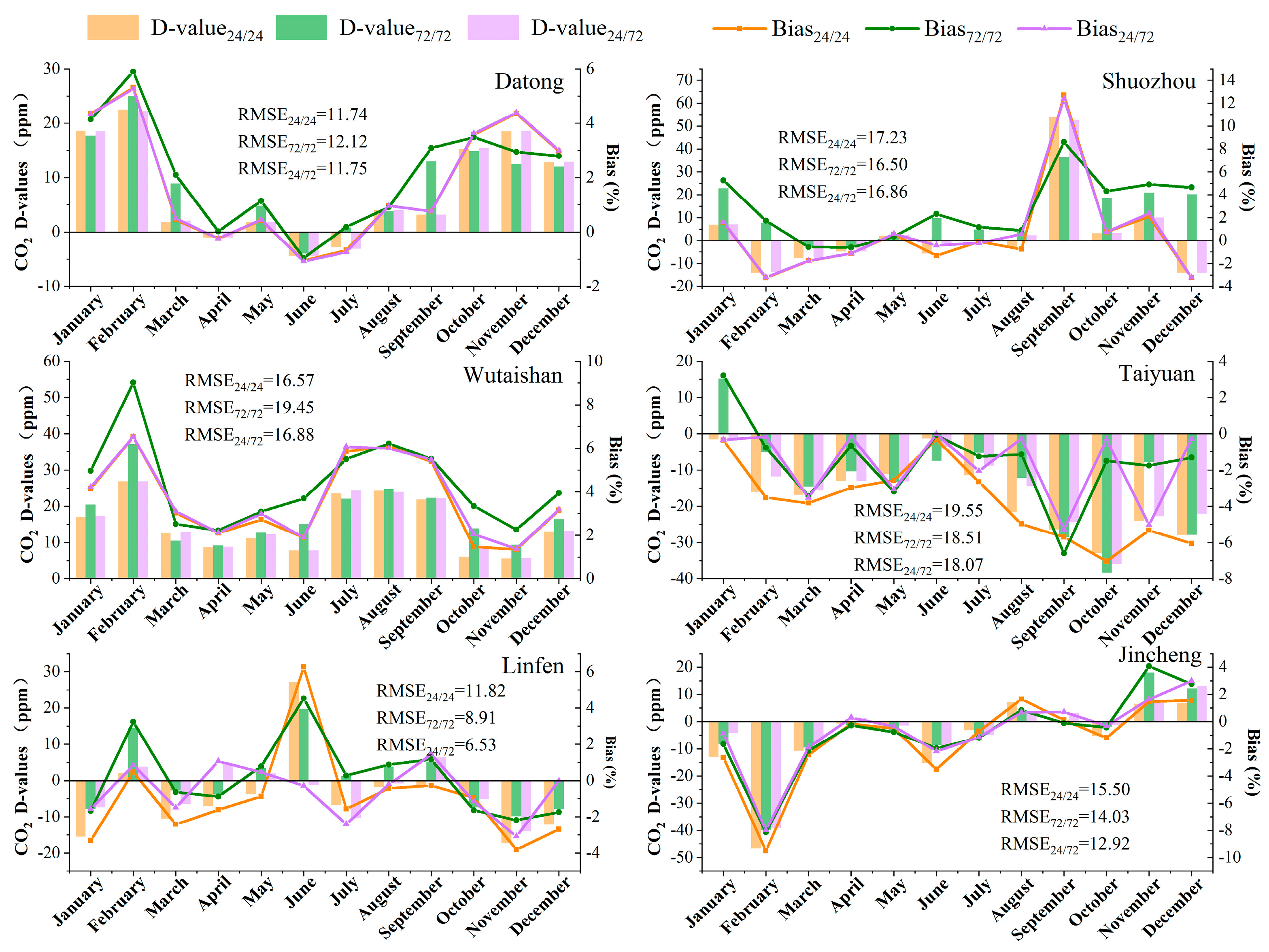
3.2. Sensitivity to the Trajectory Calculation Duration

In this section, we set the trajectory calculation altitude parameter to below 2 km. Then, we try to select the trajectory calculation duration parameter. After referring to Liu et al. [10], the trajectory calculation duration is categorized into three groups for cross-validation, namely, 24 h for both forward and backward trajectories, 72 h for both forward and backward trajectories, and 24 h for the forward trajectory and 72 h for the backward trajectory (Figure 3).
The optimal parameter experiment for the trajectory calculation duration is conducted by using the monthly averages of the observations from the six stations in 2017. By comparing the differences between the mapped values and the online observations in each month at the six stations, it is evident that although there are slight differences among the stations, the three groups of trajectory calculation durations at all six stations exhibit better-mapped results during the warm summer months (April to September) compared with the cold winter months (October to the next March). This may be related to the fact that the variations in the CO2 concentration at each station during the summer months are smaller than those during the winter months.
A comparison of the three groups’ D−value24/24, D−value72/72 and D−value24/72 shows that Linfen, Shuozhou and Jincheng stations have the largest D−value24/24, while Taiyuan, Datong and Wutaishan stations have the largest D−value72/72. Overall, the mapped values obtained by selecting a forward trajectory calculation duration of 24 h and a backward trajectory calculation duration of 72 h are closer to the in situ information. From the comparison of Bias24/24, Bias72/72 and Bias24/72 among the six stations, it is evident that the Bias24/72 values at Taiyuan, Linfen, Jincheng and Shuozhou stations are obviously better than the corresponding Bias24/24 and Bias72/72 values. However, for Datong and Wutaishan stations, the difference between Bias24/72 and Bias24/24 is not substantial, but both are noticeably better than Bias72/72. By comparing RMSE24/24, RMSE72/72 and RMSE24/72 among the six stations, it is obvious that Taiyuan, Linfen and Jincheng stations have the most optimal RMSE24/72 values. For Datong and Wutaishan stations, there is little difference between RMSE24/72 and RMSE24/24, but both are superior to RMSE72/72. For Shuozhou station, the difference between RMSE24/72 and RMSE72/72 is minor, but both outperform RMSE24/24. Comprehensively considering the three indicators that characterize the degree of difference between the mapped values and observed data from different aspects, this study selects a forward trajectory calculation duration of 24 h and a backward trajectory calculation duration of 72 h as the optimal choice for trajectory calculation duration, which minimizes the difference between the mapped results and the online observations.

4. Results and Discussion

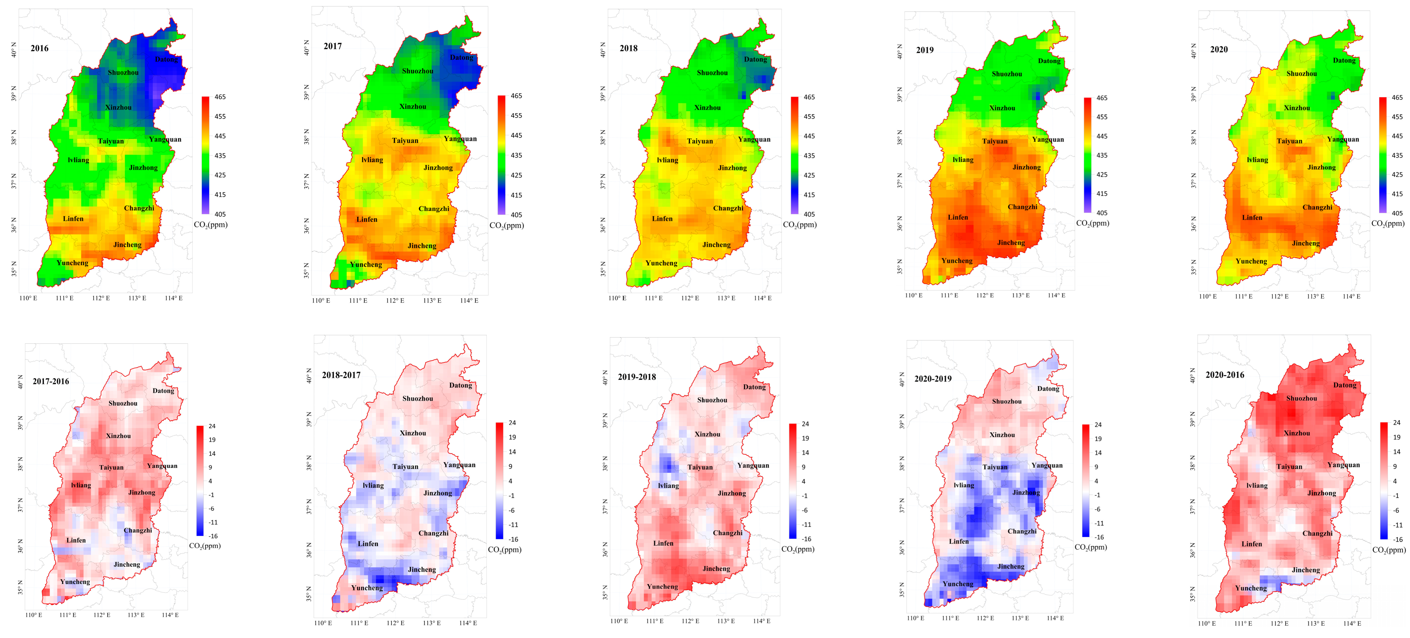
4.1. Spatio-Temporal Variation Characteristics of CO2 Concentration in Shanxi Province

Based on the 5-year online observed CO2 concentrations from the six stations, the trajectory-mapped spatial domain-filling technique is utilized to map the data from the six stations onto the entire Shanxi Province, thus deriving the distribution characteristics of the CO2 concentration across the province. The relevant parameter settings are in accordance with the results in Section 3. That is, the trajectory calculation altitude is set to less than 2 km, and the forward and backward trajectory calculation durations are set to 24 h and 72 h, respectively. Table 2 shows the average, maximum and minimum CO2 concentrations in Shanxi Province and each city from 2016 to 2020 in comparison with the global CO2 concentration and those at the background stations, and it also demonstrates the annual variation rate of CO2 concentration at each station during the 5-year period. The Waliguan global atmospheric background station serves as a representative of the background level of atmospheric CO2 in the Eurasian hinterland, while the Shangdianzi regional atmospheric background station represents the background level of CO2 concentration in North China [20]. Figure 4 illustrates the distribution of CO2 concentrations in the 11 cities across Shanxi Province from 2016 to 2020, along with the annual variations in CO2 concentrations in the entire province during the 5-year period.
As can be seen, during the five years, the provincial average CO2 concentration shows an overall upward trend, similar to the variation trends of the global CO2 concentration and those at regional background stations. Additionally, the annual average CO2 concentration in the entire province exceeds the global one and those at the two background stations. The CO2 concentration in the entire province increases from the north to the south. The low-value areas are located in Xinzhou, Datong and Shuozhou, where the CO2 concentration is comparable to or even lower than the background level in North China. The high-value areas are distributed in eastern Jincheng, northeastern Yuncheng, southeastern Changzhi, southern Linfen and southern Taiyuan, where the CO2 concentration exceeds 440.0 ppm and is substantially higher than the CO2 global concentration and at the two background stations.
Previous studies have shown that a highly developed economy, larger shares of the secondary industry and greater economic openness contribute to an elevated regional CO2 concentration [2,21]. In terms of Shanxi Province in 2020, Jincheng, Linfen, Changzhi, Taiyuan and Yuncheng, which are the areas with high CO2 concentrations, are far ahead in the gross domestic product (GDP) ranking of the entire province. The total GDP of the five cities accounts for 59% of the total GDP of the 11 cities across the province. In Jincheng, Linfen and Changzhi, where the CO2 concentration ranks in the top three, the secondary industry shares all exceed 43%. However, in Datong, Yangquan and Xinzhou, where the CO2 concentration is low, the GDPs are below the provincial average [22]. Additionally, a higher population density leads to larger infrastructure development [23], larger traffic volume and more combustion of heating fuels [24,25], thus resulting in higher CO2 emissions [26]. This is also a reason for the higher CO2 concentration in the cities with a higher population density, such as Taiyuan and Yuncheng. In contrast, Xinzhou has the lowest population density in Shanxi Province and is less influenced by human activities [22]. As a result, these cities exhibit relatively lower CO2 concentrations (the table for GDP and population density distribution in each city in Shanxi Province is omitted). In addition, the results of the Shanxi carbon emission inversion in 2020 based on China Carbon Monitoring and Verification Support (CCMVS) show that Linfen has the highest carbon emissions of 46.2 TgCy−1, accounting for 26% of the total carbon emissions in the province, which is in the second place of the high-value areas of CO2 concentration in the province; while Xinzhou has the smallest carbon emissions of 3.4 TgCy−1, accounting for 2% of the total carbon emissions in the province, which is the second lowest area in terms of CO2 concentration in the province [27].
This study also analyzes the annual variation oinCO2 concentration. From the comparison of two consecutive years, it can be found that during the years with CO2 concentration growth, the variation rate is the largest in 2019 relative to 2018, substantially exceeding the variation rate of the global CO2 concentration and those at background stations observed in the Eurasian hinterland and North China. Only central Lvliang and a very few low-value areas in Xinzhou show a declining trend of CO2 concentration, while the rest of the region exhibits an increasing trend, particularly in the conjunction area of Jinzhong, Linfen and Yuncheng, where the CO2 concentration increases significantly. The variation rate is the smallest in 2018 relative to 2017, dramatically lower than the variation rate of the global CO2 concentration and those of background stations. Taiyuan, Jinzhong, Linfen and Yuncheng, where the CO2 concentration is high, show a noticeable decreasing trend of CO2 concentration. However, the low-value areas of CO2 concentration such as Xinzhou, Datong and Shuozhou, exhibit an increasing trend. Different from the variation rate of the global CO2 concentration and those at the two background stations, the CO2 concentration in Shanxi Province experienced a negative variation rate of CO2 concentration in 2020 relative to 2019, which is the only year with a negative variation rate among several comparative years. This can be attributed to the swift and thorough preventive and control measures that were implemented by the government during the COVID-19 pandemic in 2020, and these measures led to a slowdown in economic growth and a reduction in urban CO2 emissions. According to the Shanxi Statistical Yearbook, the annual GDP growth rate in the entire province in 2020 was 3.6%, substantially lower than the average of 5.9% in the previous four years (2016–2019) [22]. Additionally, according to the Global Carbon Project, global daily CO2 emissions decreased by as much as 17% compared with those in 2019 during the most intense period of mandatory lockdowns in early 2020. It is estimated that the annual CO2 emissions in 2020 decreased by 4.2–7.5% compared with those in 2019 [28,29]. The reduction is particularly pronounced in urban areas, but it does not have an impact on the global average CO2 concentration. In 2020, the variations in the CO2 concentration in the low-value areas of Datong, Shuozhou and Xinzhou in Shanxi Province were the same as the global ones and those at the two background stations. These areas are less affected by human activities and thus show a positive variation rate, and the CO2 concentration increases year on year. In contrast, the remaining eight cities with a high CO2 concentration show a year-on-year decreasing trend of CO2 concentration. These areas are greatly influenced by economic development. Specifically, the reduction in CO2 concentration is the most prominent in Yuncheng, Jinzhong and Jincheng.
To further analyze the overall variation characteristics of the CO2 concentration in Shanxi Province during the 13th Five-Year Plan period, a comparative analysis of the CO2 concentration in the entire province and the 11 cities between 2020 and 2016 is conducted (Figure 4). The average CO2 concentration variation rate in Shanxi Province was 2.12% in 2020 relative to 2016, which is between the variation rates of the Waliguan and global CO2 concentration (2.45%) and Shangdianzi CO2 concentration (1.81%). During the 5-year period, the increment of CO2 concentration shows an overall decreasing trend from the north to the south across the province. The increments of CO2 concentration in the northern regions of Datong, Shuozhou and Xinzhou were the largest, with a variation rate exceeding 3.4%. However, the variation rates of the CO2 concentration in the southern-central regions were all below 2.3%, indicating a relatively lower growth of CO2 concentration. The gap of CO2 concentration between the high-value and low-value areas was narrower in 2020 than in 2016. During the five years, the CO2 concentration increased faster in the northern low-value areas than in the southern high-value areas, which may be related to the fact that northern ecosystems are experiencing large changes in vegetation and carbon cycle dynamics. Matthias et al. [30] analyzed the variation characteristics of atmospheric CO2 in the Northern Hemisphere in the last 40 years and also found that the increase in CO2 at high latitudes is more intensive than at low latitudes.

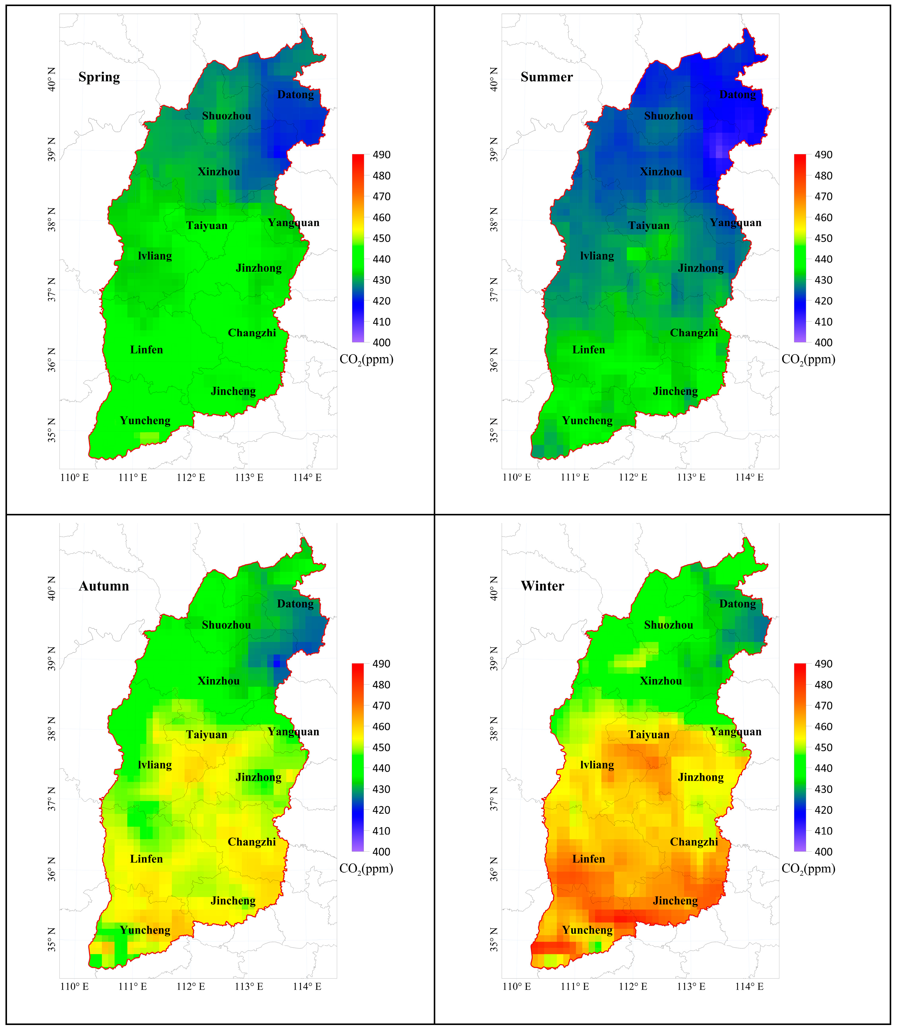
4.2. Seasonal Variation Characteristics of CO2 Concentration in Shanxi Province

The distribution of CO2 concentration in Shanxi Province exhibits seasonal variations due to the seasonal variations of atmospheric CO2 sources and sinks, including carbon uptake and emission of terrestrial ecosystems and anthropogenic carbon emission, as well as the atmospheric seasonal oscillation [31]. Figure 5 shows that the CO2 concentration in the entire province in spring and summer was lower than that in autumn and winter during 2016–2020. The mean values in spring, summer, autumn and winter are (433.6 ± 4.6) ppm, (427.7 ± 4.9) ppm, (445.8 ± 7.8) ppm and (453.3 ± 10.7) ppm, respectively. The maximum CO2 concentration appears in eastern Yuncheng in winter with the value of 485.3 ppm, and the minimum occurs in northeastern Xinzhou in summer with the value of 407.2 ppm. In autumn, the wind speed is relatively low, the atmospheric stratification is stable [32], and the atmospheric vertical motion is weak. Thus, the CO2 is difficult to disperse and accumulates near the surface. In winter, the daytime hours are shorter, plants decay, and the photosynthesis of the ecosystem weakens greatly. As a consequence, an essential CO2 sink is lost. Meanwhile, the lower temperature and lower boundary layer height increase the frequency of temperature inversions, further hindering CO2 diffusion. Moreover, the heating demand of people during winter in northern regions increases CO2 emissions [15]. The combined effects of these factors result in a higher CO2 concentration during autumn and winter. On the contrary, during spring, there is a higher wind speed and a higher boundary layer height, accompanied by enhanced vertical motion. These factors jointly facilitate CO2 diffusion. Additionally, the longer daylight hours and enhanced plant photosynthesis also contribute to CO2 uptake. In summer, because of abundant vegetation, ample sunlight and higher temperatures, plant photosynthesis is more vigorous compared with that under lower temperatures. Approximately 30% of the CO2 emitted from fossil fuel combustion can be absorbed by plants, and thus, an essential CO2 sink is generated [33,34]. The combined effects of these factors lead to a lower CO2 concentration during spring and summer. The analysis above is consistent with the seasonal variations in CO2 concentration that are observed in other regions in the Northern Hemisphere [35].
The seasonal amplitudes of the CO2 concentration in spring, summer, autumn and winter are 30.5 ppm, 33.1 ppm, 46.8 ppm and 59.4 ppm, respectively, and the amplitudes in spring and summer are smaller than those in autumn and winter. Throughout all four seasons, the CO2 concentration increases from the north to the south. In the northern regions, especially in northeastern Xinzhou, the CO2 concentration remains at a relatively low level throughout the year, with a smaller seasonal amplitude of around 20 ppm. In contrast, the southern-central regions exhibit a relatively higher CO2 concentration throughout the year, with a larger seasonal amplitude of around 30 ppm. This finding is consistent with most previous studies in mid-latitude regions [36].
The seasonal average RMSE between the mapped and observed values at the six stations is 4.72 ppm. This value is lower than the RMSE (5 ppm) between the highly consistently observed CO2 concentrations by two instruments, reported by Liu et al. [37]. This further confirms that it is feasible to derive the distribution characteristics of CO2 concentration in the entire province by employing the trajectory-mapped spatial domain-filling technique based on the existing CO2 concentration data from the six observation stations in Shanxi province.

5. Conclusions

In this study, the trajectory mapping domain-filling technology, which can provide more reliable statistical estimates of long-lived gas concentrations in a broader geographical area based on limited station data, is used innovatively for mapping the CO2 concentration data of six ground observation stations to the whole Shanxi province. It solves the problem of the limited spatial coverage of greenhouse gas observations, which limits the comprehensive understanding of the regional CO2 distribution characteristics, realizes the data from “point” to “surface”, and helps obtain the spatio-temporal distribution characteristics of CO2 in the whole Shanxi region.
The results of this study on the inter-annual variations in CO2 concentration in the entire province show that the highest year-on-year increase occurred in 2019, while the lowest year-on-year increase appeared in 2018. However, according to the Shanxi Statistical Yearbook, the GDP growth rate of the entire province was 6.1% in 2019 and 6.6% in 2018, indicating that reducing CO2 emissions does not necessarily require sacrificing economic development. In 2018, despite steady economic growth in Shanxi, there was a relatively small increase in CO2 concentration. This can be attributed to effective control measures being implemented in the areas with high CO2 concentrations. The targeted reduction in emissions from high-emission cities resulted in an overall decrease in CO2 emissions in the entire region. By comprehensively comparing the year-by-year variations, it can be seen that in the year with a low increment or even a negative increment of maximum value, the overall CO2 concentration in the entire province did not increase sharply. The key to carbon reduction lies in the control of CO2 in high-value areas. Developing targeted emission reduction policies in these high-value areas is crucial, and the control measures in the high-value areas are the core of carbon reduction.
Furthermore, this study indicates that there are distinct spatio-temporal differences in CO2 concentration in Shanxi Province, which are closely related to regional emissions. Reducing emissions is the fundamental pathway to achieving carbon neutrality, and precise control of CO2 emission sources is especially important. Based on the spatio-temporal distribution characteristics of the CO2 concentration in the 11 cities of Shanxi Province presented in this study, further information extraction of CO2 emission sources and the identification of emission source strengths will enable a better understanding of the key aspects of carbon reduction. This will provide essential data support for the formulation of more precise emission reduction policies with regional relevance in Shanxi Province.

Author Contributions

Conceptualization, S.Y. and F.Z.; methodology, S.Y. and F.Z.; software, S.Y. and F.Z.; validation, X.G., K.P. and L.S.; formal analysis, F.Z; investigation, Y.L. and Y.W.; resources, K.P. and Y.L.; data curation, F.Z. and L.S.; writing—original draft preparation, F.Z.; writing—review and editing, F.Z. and X.G.; visualization, F.Z. and X.G; supervision, S.Y. and L.Z.; project administration, A.Y. and H.S.; funding acquisition, H.S., F.Z., Y.L. and L.Z. All authors have read and agreed to the published version of the manuscript.

Funding

This study was supported by the National Key Research and Development Program (2019YFC1510304), the Basic Research Program of Shanxi (202203021212112 and 20210302124617), the Innovation Development Special project of China Meteorological Administration (CXFZ2023P022), and the Central Guide Local Science and Technology Development Funds Specia (YDZJSX2021B17).

Institutional Review Board Statement

Not applicable.

Informed Consent Statement

Not applicable.

Data Availability Statement

The data are not available due to restrictions. The participants have not consented to the data being shared.

Acknowledgments

The authors wish to acknowledge the anonymous reviewers for their detailed and helpful comments on the original manuscript. We are grateful to the staff of the greenhouse gas observation network in Shanxi Province for their daily maintenance of the online greenhouse gas observation system. We also thank Nanjing Hurricane Translation for reviewing the English language quality of this paper. The authors thank the experts for their review. We would also like to thank the NOAA Air Resources Laboratory (ARL) for providing the HYSPLIT4 model.

Conflicts of Interest

The authors declare no conflict of interest.

References

  1. IPCC. Climate Change 2021: The Physical Science Basis; The Working Group I Contribution to the Sixth Assessment Report of the Intergovernmental Panel on Climate Change; IPCC: Geneva, Switzerland, 2021. [Google Scholar]
  2. Zhang, F.; Xuan, X.; Deng, X.Z. Research progress and prospect on the non-uniform distribution of atmospheric CO2 concentration and its influence on surface warming. J. Geo-Inf. Sci. 2021, 23, 1362–1371. [Google Scholar]
  3. Shan, Y.; Guan, D.; Zheng, H.; Ou, J.; Li, Y.; Meng, J.; Mi, Z.; Liu, Z.; Zhang, Q. Data descriptor: China CO2 emission accounts 1997–2015. Sci. Data 2018, 5, 170201. [Google Scholar] [CrossRef]
  4. Shan, Y.; Huang, Q.; Guan, D.; Hubacek, K. China CO2 emission accounts 2016–2017. Sci. Data 2020, 7, 54. [Google Scholar] [CrossRef]
  5. Liu, L.; Tans, P.P.; Xia, L.; Zhou, L.; Zhang, F. Analysis of patterns in the concentrations of atmospheric greenhouse gases measured in two typical urban clusters in China. Atmos. Environ. 2018, 173, 343–354. [Google Scholar] [CrossRef]
  6. Newman, S.; Jeong, S.; Fischer, M.L.; Xu, X.; Haman, C.L.; Lefer, B.; Alvarez, S.; Rappenglueck, B.; Kort, E.A.; Andrews, A.E.; et al. Diurnal tracking of anthropogenic CO2 emissions in the Los Angeles basin megacity during spring 2010. Atmos. Chem. Phys. 2013, 13, 4359–4372. [Google Scholar] [CrossRef]
  7. Lan, L.; Ghasemifard, H.; Yuan, Y.; Hachinger, S.; Zhao, X.; Bhattacharjee, S.; Bi, X.; Bai, Y.; Menzel, A.; Chen, J. Assessment of Urban CO2 Measurement and Source Attribution in Munich Based on TDLAS-WMS and Trajectory Analysis. Atmosphere 2020, 11, 58. [Google Scholar] [CrossRef]
  8. Wei, C.; Wang, M.; Fu, Q.; Dai, C.; Huang, R.; Bao, Q. Temporal Characteristics of Greenhouse Gases (CO2 and CH4) in the megacity Shanghai, China: Association with air pollutants and meteorological conditions. Atmos. Res. 2020, 235, 104759. [Google Scholar] [CrossRef]
  9. Wei, F.; Lin, H.; Cao, S.; Shen, P.; Hui, P. A study on background concentration and source-sink characteristics of CO2 in south of Jiangsu. China Environ. Sci. 2020, 40, 975–982. [Google Scholar]
  10. Liu, J.; Tarasick, D.W.; Fioletov, V.E.; McLinden, C.; Zhao, T.; Gong, S.; Sioris, C.; Jin, J.J.; Liu, G.; Moeini, O. A global ozone climatology from ozone soundings via trajectory mapping: A stratospheric perspective. Atmos. Chem. Phys. 2013, 13, 11441–11464. [Google Scholar] [CrossRef]
  11. Liu, G.; Liu, J.; Tarasick, D.W.; Fioletov, V.E.; Jin, J.J.; Moeini, O.; Liu, X.; Sioris, C.E.; Osman, M. A global tropospheric ozone climatology from trajectory-mapped ozone soundings. Atmos. Chem. Phys. 2013, 13, 10659–10675. [Google Scholar] [CrossRef]
  12. Xu, W.; Xu, X.; Lin, M.; Lin, W.; Tarasick, D.; Tang, J.; Ma, J.; Zheng, X. Long-term trends of surface ozone and its influencing factors at the Mt Waliguan GAW station, China-Part 2: The roles of anthropogenic emissions and climate variability. Atmos. Chem. Phys. 2018, 18, 773–798. [Google Scholar] [CrossRef]
  13. Zhang, F.; Zhu, L.; Yan, S.; Gao, X.A.; Pei, K. Analysis of the CO2 Mole Fraction Variation and its Transmission Characteristics in Taiyuan. Atmos. Ocean. Sci. Lett. 2020, 13, 363–370. [Google Scholar] [CrossRef]
  14. Morris, G.A.; Gleason, J.F.; Ziemke, J.; Schoeberl, M.R. Trajectory mapping: A tool for validation of trace gas observations. J. Geophys. Res. 2000, 105, 17875–17894. [Google Scholar] [CrossRef]
  15. Bezyk, Y.; Sówka, I.; Górka, M.; Blachowski, J. GIS-Based approach to spatio-temporal interpolation of atmospheric CO2 concentrations in limited monitoring dataset. Atmosphere 2021, 12, 384. [Google Scholar] [CrossRef]
  16. Osman, M.K.; Tarasick, D.W.; Liu, J.; Moeini, O.; Thouret, V.; Fioletov, V.E.; Parrington, M.; Nédélec, P. Carbon monoxide climatology derived from the trajectory mapping of global MOZAIC-IAGOS data. Atmos. Chem. Phys. 2016, 16, 10263–10282. [Google Scholar] [CrossRef]
  17. Yan, S.; Gao, X.; Pei, K.; Sun, H.; Wang, Y.; Zhang, F.; Li, Y.; Wang, S.; Chen, L.; Dong, J.; et al. Mixing-layer depth-based backwards trajectory analysis of the sources of high O3 concentrations at the Wutaishan station, North China. Atmos. Pollut. Res. 2023, 14, 11652. [Google Scholar] [CrossRef]
  18. Al-Mamoori, S.K.; Al-Maliki, L.A.; Al-Sulttani, A.H.; El-Tawil, K.; Al-Ansari, N. Statistical analysis of the best GIS interpolation method for bearing capacity estimation in An-Najaf City, Iraq. Environ. Earth Sci. 2021, 80, 683. [Google Scholar] [CrossRef]
  19. Wei, F. Modern Climate Statistical Diagnosis and Prediction Techniques; China Meteorlogical Press: Beijing, China, 2022; pp. 18–41. [Google Scholar]
  20. Zhang, L.; Meng, J.G.; Liu, Y.F.; Liang, X.; Yang, S.Q.; Xian, Y. Concentration variation characteristics of atmospheric greenhouse gases at Waliguan and Shangdianzi in China. Earth Sci. 2021, 46, 2984–2998. [Google Scholar]
  21. Zhao, L.; Wu, D. Carbon emission accounting and spatial heterogeneity pattern of China’s energy supply side. China Popul. Resour. Environ. 2018, 28, 48–58. [Google Scholar]
  22. Shanxi Provincial Bureau of Statistics. 2017–2021. Survey Office of the National Bureau of Statistics in Shanxi; Shanxi Statistical Yearbook; China Statistics Press: Beijing, China, 2022. [Google Scholar]
  23. Bergeron, O.; Strachan, I.B. CO2 sources and sinks in urban and suburban areas of a northern mid-latitude city. Atmos. Environ. 2011, 45, 1564–1573. [Google Scholar] [CrossRef]
  24. Park, C.; Jeong, S.; Park, M.S.; Park, H.; Yun, J.; Lee, S.S.; Park, S.H. Spatiotemporal variations in urban CO2 flux with land-use types in Seoul. Carbon Balance Manag. 2022, 17, 3. [Google Scholar] [CrossRef] [PubMed]
  25. Matthews, B.; Schume, H. Tall tower eddy covariance measurements of CO2 fluxes in Vienna, Austria. Atmos. Environ. 2022, 274, 118941. [Google Scholar] [CrossRef]
  26. Górka, M.; Lewicka-Szczebak, D. One-year spatial and temporal monitoring of concentration and carbon isotopiccomposition of atmospheric CO2 in a Wrocław (SW Poland) city area. Appl. Geochem. 2013, 35, 7–13. [Google Scholar] [CrossRef]
  27. Guo, L.; Zhang, X.; Zhong, J.; Wang, D.; Miao, C.; Zhao, L.; Zhou, Z.; Liao, J.; Hu, B.; Zhu, L.; et al. Construction and application of a regional kilometer-s carbon sourceand sink assimilation inversion system (CCMVS-R). Engineering 2023, in press. [Google Scholar] [CrossRef]
  28. WMO/GAW. WMO Greenhouse Gas Bulletin: The State of Greenhouse Gases in the Atmosphere Based on Global Observations through 2019; WMO/GAW: Geneva, Switzerland, 2020. [Google Scholar]
  29. Le Quéré, C.; Jackson, R.B.; Jones, M.W.; Smith, A.J.; Abernethy, S.; Andrew, R.M.; De-Gol, A.J.; Willis, D.R.; Shan, Y.; Canadell, J.G.; et al. Temporary reduction in daily global CO2 emissions during the COVID-19 forced confinement. Nat. Clim. Chang. 2020, 10, 647–653. [Google Scholar] [CrossRef]
  30. Forkel, M.; Carvalhais, N.; Rödenbeck, C.; Keeling, R.; Heimann, M.; Thonicke, K.; Zaehle, S.; Reichstein, M. Enhanced seasonal CO2 exchange caused by amplified plant productivity in northern ecosystems. Science 2016, 351, 696–699. [Google Scholar] [CrossRef]
  31. Huang, X. Characteristics of Atmospheric Carbon Dioxide in urban Area and the Influence of the Regionally Inhomogeneously Distribution on Climate. Ph.D. Thesis, Nanjing University, Nanjing, China, 2015. [Google Scholar]
  32. Yurkov, I.A.; Dzholumbetov, S.K.; Gulyaev, E.A. Estimation of Nocturnal Greenhouse Gas Emissions in Yekaterinburg in 2018–2019. Russ. Meteorol. Hydrol. 2021, 46, 768–774. [Google Scholar] [CrossRef]
  33. Schimel, D.; Stephens, B.B.; Fisher, J.B. Effect of increasing CO2 on the terrestrial carbon cycle. Proc. Natl. Acad. Sci. USA 2015, 112, 436–441. [Google Scholar] [CrossRef]
  34. Wang, Q.; Imasu, R.; Arai, Y.; Ito, S.; Mizoguchi, Y.; Kondo, H.; Xiao, J. Sub-Daily Natural CO2 Flux Simulation Based on Satellite Data: Diurnal and Seasonal Pattern Comparisons to Anthropogenic CO2 Emissions in the Greater Tokyo Area. Remote Sens. 2021, 13, 2037. [Google Scholar] [CrossRef]
  35. Huang, X.; Wang, T.; Talbot, R.; Xie, M.; Mao, H.; Li, S.; Zhuang, B.; Yang, X.; Fu, C.; Zhu, J.; et al. Temporal characteristics of atmospheric CO2 in urban Nanjing, China. Atmos. Res. 2015, 153, 437–450. [Google Scholar] [CrossRef]
  36. Wang, P.; Zhou, W.; Niu, Z.; Xiong, X.; Wu, S.; Cheng, P.; Hou, Y.; Lu, X.; Du, H. Spatio-temporal variability of atmospheric CO2 and its main causes: A case study in Xi’an city, China. Atmos. Res. 2021, 249, 105346. [Google Scholar] [CrossRef]
  37. Liu, D.; Sun, W.; Zeng, N.; Han, P.; Yao, B.; Liu, Z.; Wang, P.; Zheng, K.; Mei, H.; Cai, Q. Observed decreases in on-road CO2 concentrations in Beijing during COVID-19 restrictions. Atmos. Chem. Phys. 2021, 21, 4599–4614. [Google Scholar] [CrossRef]
Figure 1. Schematic diagram of the GHG observation network in Shanxi Province of China.
Atmosphere 15 00098 g001
Figure 2. Comparison of CO2 mapped values at different trajectory calculation altitudes with the seasonal averages of the in situ information at the six stations in Shanxi from 2016 to 2020. (The black line represents the 1:1 line. The differently colored dots denote different trajectory altitudes, with red dots indicating all altitudes reachable by the trajectory model (the “all” group), green dots indicating altitudes below 2 km (the “down” group), and blue dots indicating altitudes above 2 km (the “top” group). The variable N represents the total number of data, with 20 data points in total over five years. Rall, Rdown and Rtop denote the correlation coefficients of the mapped values’ trajectory calculation altitude to the in situ information at corresponding trajectory calculation altitudes. When N = 20, α = 0.001, Rxt = 0.652; α = 0.01, Rxt = 0.537; α = 0.1, Rxt = 0.360 [19]. RMSEall, RMSEdown and RMSEtop represent the root mean square errors (RMSEs) of the mapped values at corresponding trajectory calculation altitudes with the online observations. The values range from 0 to +∞, and the values closer to 0, indicate a more perfect fit. Biasall, Biasdown and Biastop are the relative biases of the mapped values at corresponding trajectory calculation altitudes with the online observations, and the values closer to 0 indicate a more perfect fit).
Atmosphere 15 00098 g002
Figure 3. Comparison of CO2 mapped values under different trajectory calculation durations with the monthly averages of the in situ information at the six stations in Shanxi in 2017. The orange, green and purple bar charts correspond to D−value24/24, D−value72/72 and D−value24/72, respectively, which indicate the differences between the CO2 mapped values at corresponding trajectory calculation duration and the in situ information. The orange, green and purple line charts correspond to Bias24/24, Bias72/72 and Bias24/72, respectively, representing the relative biases of the mapped values at corresponding trajectory calculation duration with the in situ information. Similarly, RMSE24/24, RMSE72/72, and RMSE24/72 represent the root mean square errors of the mapped values at corresponding trajectory calculation duration with the in situ information.
Atmosphere 15 00098 g003
Figure 4. Spatio−temporal distribution characteristics of CO2 concentration in Shanxi from 2016 to 2020.
Atmosphere 15 00098 g004
Figure 5. Seasonal variation characteristics of CO2 concentration in Shanxi.
Atmosphere 15 00098 g005
Table 1. Overview of the six stations in the GHG observation network in Shanxi.
StationAltitude (m)Surrounding Environment
Datong1052.6The station is located within the Datong national basic meteorological station, with the surrounding area primarily composed of farmland. To the west, there are expressways, while to the east, there are railways and the G109 national road.
Shuozhou1114.8The station is within the Shuozhou national basic meteorological station, situated in the north of the downtown. The surrounding area mainly consists of enterprises, institutions, residential areas and urban transportation routes, with relatively sparse vegetation.
Wutaishan2208.3The station is within the Wutaishan national basic meteorological station and is located at the top of Wutaishan Mountain. Within a radius of 30 km, there are no large cities or industrial areas. The surrounding area is mainly covered by forests and grasslands.
Taiyuan776.2The station is within the Xiaodian national ordinary meteorological station, situated to the south of the downtown. It is adjacent to the urban expressway and the Beijing–Kunming Expressway. The surrounding area has a high population density and relatively sparse vegetation.
Linfen449.5The station is within the Linfen national basic meteorological station, located in the southwestern part of the downtown. The surrounding area has complex road networks, a high population density and relatively sparse vegetation.
Jincheng752.6The station is situated in the northern part of the downtown, to the south of the Baimasi Botanical Garden, and is adjacent to a middle school and a provincial road.
Table 2. Comparison of average CO2 concentrations in Shanxi Province and the 11 cities during 2016–2020 with global and two background stations.
YearAnnual Concentrations (ppm)Variation Rate (%)
Area 201620172018201920202017–20162018–20172019–20182020–20192020–2016
Global403.3 ± 0.1405.5 ± 0.1407.8 ± 0.1410.5 ± 0.2413.2 ± 0.20.550.570.660.662.45
WLG404.4 ± 0.9407.0 ± 0.2409.4 ± 0.3411.4 ± 0.3414.3 ± 0.20.640.590.490.702.45
SDZ413.7 ± 1.0416.0 ± 1.8421.6 ± 1.5420.4 ± 1.9421.2 ± 0.20.561.35−0.280.191.81
Shanxi433.3 ± 8.5438.2 ± 7.9438.6 ± 6.2443.7 ± 8.1442.5 ± 5.41.130.091.16−0.272.12
Datong419.0 ± 3.5422.2 ± 3.0425.5 ± 2.9432.6 ± 3.0433.3 ± 3.10.760.781.670.163.41
Shuozhou423.2 ± 2.2426.5 ± 2.2429.7 ± 1.9432.4 ± 1.9438.1 ± 2.40.780.750.631.323.52
Xinzhou422.4 ± 4.6428.4 ± 4.7431 ± 3.1432.6 ± 3.1437.3 ± 3.71.420.610.371.093.53
Taiyuan435.2 ± 3.9443.8 ± 3.9442.9 ± 2.9448.2 ± 5.0444.9 ± 4.01.98−0.201.20−0.742.23
Yangquan428.5 ± 4.5436.6 ± 2.6437.4 ± 2.1438.3 ± 2.2436.9 ± 1.51.890.180.21−0.321.96
Lvliang434.8 ± 2.6442.7 ± 3.1442.2 ± 3.1443.8 ± 3.7442.1 ± 2.81.82−0.110.36−0.381.68
Jinzhong435.3 ± 2.7443.7 ± 1.9442.6 ± 2.1448.5 ± 2.8443.3 ± 3.41.93−0.251.33−1.161.84
Changzhi441.3 ± 3.9443.8 ± 2.4445 ± 2.3449.8 ± 2.6447.7 ± 4.10.570.271.08−0.471.45
Linfen443.2 ± 2.6445.7 ± 2.9444.8 ± 2.2452.8 ± 3.0450.2 ± 3.50.56−0.201.80−0.571.58
Jincheng448.5 ± 2.9448.6 ± 2.6445.9 ± 2.1455.4 ± 2.2450.7 ± 3.20.02−0.602.13−1.030.49
Yuncheng439.6 ± 6.9442.9 ± 6.7441.3 ± 2.4451.8 ± 4.4444.2 ± 2.50.75−0.362.38−1.681.05
Disclaimer/Publisher’s Note: The statements, opinions and data contained in all publications are solely those of the individual author(s) and contributor(s) and not of MDPI and/or the editor(s). MDPI and/or the editor(s) disclaim responsibility for any injury to people or property resulting from any ideas, methods, instructions or products referred to in the content.

