Spatial–Temporal Temperature Forecasting Using Deep-Neural-Network-Based Domain Adaptation

Abstract

Accurate temperature forecasting is critical for various sectors, yet traditional methods struggle with complex atmospheric dynamics. Deep neural networks (DNNs), especially transformer-based DNNs, offer potential advantages, but face challenges with domain adaptation across different geographical regions. We evaluated the effectiveness of DNN-based domain adaptation for daily maximum temperature forecasting in experimental low-resource settings. We used an attention-based transformer deep learning architecture as the core forecasting framework and used kernel mean matching (KMM) for domain adaptation. Domain adaptation significantly improved forecasting accuracy in most experimental settings, thereby mitigating domain differences between source and target regions. Specifically, we observed that domain adaptation is more effective than exclusively training on a small amount of target-domain training data. This study reinforces the potential of using DNNs for temperature forecasting and underscores the benefits of domain adaptation using KMM. It also highlights the need for caution when using small amounts of target-domain data to avoid overfitting. Future research includes investigating strategies to minimize overfitting and to further probe the effect of various factors on model performance.

1. Introduction

Temperature forecasting has seen significant advancements driven by the necessity to accurately predict weather patterns for various sectors, including agriculture, energy, and disaster management. Traditional methods have relied heavily on statistical models and physical principles, which, while effective, are often unable to capture the complex non-linear relationships inherent in atmospheric dynamics [1]. Recent advances in machine learning, especially the development of deep neural networks (DNNs), have opened up new possibilities for improving the accuracy of temperature forecasting [2].

DNNs have demonstrated remarkable success in various domains, including natural language processing, computer vision, speech processing, and even weather forecasting [2,3]. This success is attributed to their ability to learn complex patterns from large datasets. The transformer deep learning architecture [4] is now the state-of-the-art architecture and core of the most advanced large language models, including those based on bidirectional encoder representations from transformers (BERTs) and generative pre-trained transformers (GPTs) [5]. A transformer-based model’s ability to handle sequential data, its attention mechanism for effectively learning various internal structures, and its potential for domain adaptation make such models promising for temperature forecasting, especially in low-resource settings where domain adaptation is needed [6,7].

However, the application of DNNs, including transformer DNNs, to temperature forecasting is not without challenges. One significant hurdle is domain adaptation, given that weather patterns and their underlying dynamics can vary significantly across different geographical regions. A model trained on data from one region may therefore not perform optimally when applied to another region. Thus, domain adaptation aims to bridge this gap by resolving the domain differences between the source and target domains in terms of data and models [8,9]. This enables bringing more data and better-trained models from the source domain, especially when the target-domain data are too scarce or unavailable for training an effective model.

The scarcity of high-quality data for use in machine learning tasks such as temperature forecasting is a major concern due to several factors. Limited data availability and quality can hinder model performance and generalization, potentially leading to inaccurate predictions [9,10]. This is particularly critical in temperature forecasting, where accurate forecasts are vital for solutions related to agriculture, energy, climate change, etc. [10]. The challenge of limited data has stimulated innovation in machine learning techniques, especially domain adaptation [9,11]. Thus, the problem of data scarcity is a key area of interest in the field [9,10,11].

In one of the most recent studies on domain adaptation for time-series forecasting [11], the framework used was shown to be effective even when transferring data from a source domain to a target domain with a different signal frequency, where, in most cases, it was able to approximately capture the sinusoidal signals even when the input was contaminated by white noise. Experiments were performed on four datasets: household electricity consumption, highway traffic, daily sales of grocery stores, and daily Wikipedia visit counts. The main technique that they used, namely attention sharing via adversarial training, was inspired by the success of transformer-based DNNs and adversarial training in domain adaptation.

We have developed a DNN-based domain adaptation method designed to forecast time series. Our numerical experiments focused on the use of this method to forecast the daily maximum temperature at a finite number of locations. We are motivated to tackle the problem of forecasting the daily maximum temperature since it is strongly related to heatstroke damage mitigation, especially amid the current global climate change issue, where this heatstroke problem is becoming more severe [12,13]. The idea is to use domain adaptation to increase the forecasting power of the model in a region for which only a small amount of data is available. The model is a DNN-based model instead of a complex physical model such as those generally used by Japan meteorologists (https://www.jma.go.jp/jma/en/Activities/nwp.html, accessed on 7 March 2023). We used a different approach that utilizes DNNs and KMM, presented in the following section. Experiments were set up with scenarios of limited data for target regions in order to test our method. We compare our method with a recent advanced domain adaptation method proposed by Jin et al. (2022) [11] that was not applied to temperature forecasting. Despite the importance, domain adaptation for temperature forecasting is, unexpectedly, not yet well explored compared to other research disciplines [9].

This paper is composed of four key sections following this introductory section. Section 2 provides an in-depth presentation of our method, the data gathered, and the model used. It details the research procedures, specifies the sources and nature of the data collected, and describes the model’s formulation. Section 3 focuses on the experiments conducted, the results obtained, and the conclusions drawn from the results. It outlines the experimental design, the process undertaken, and the findings. Finally, Section 4 recapitulates the research and its key findings, restates the implications of the results, and proposes areas for future research.

2. Proposed Method

2.1. Time-Series Forecasting Problem

Suppose a set of N time series, each consisting of observations $z_{i,t}\in \mathbb{R}$ associated with optional input covariates ${\xi }_{i,t}\in {\mathbb{R}}^d$ at time t. In time-series forecasting, given T past observations, the aim for the i-th time series ${\left\{x_{i,t}\right\}}_{t=1,\dots ,T}$ and all the input covariates is to make multi-horizon future predictions at time $t\in \{T+1,\dots ,T+\tau \}$ using model H:

$$z_{i,T+1},\dots ,z_{i,T+\tau }=H(z_{i,1},\dots ,z_{i,T};{\xi }_{i,1},\dots ,{\xi }_{i,T+\tau }).$$

(1)

In our numerical experiments, we considered the daily maximum temperature of the i-th location at time t as response variable $z_{i,t}$. However, the proposed method could be easily applied to other time-series forecasting problems. The chosen covariates will be described in Section 3.1.

Here, we are particularly interested in scenarios in which only a small amount of data are available for the problem of interest while a sufficiently large amount of data is available for other related sources. Our framework for evaluating the effectiveness of our approach is illustrated in Figure 1. We denote dataset $\mathcal{D}={\left\{X_i,Y_i\right\}}_{i=1}^N$, with $X_i=\left({\left\{z_{i,t}\right\}}_{t=1}^T,{\left\{{\xi }_{i,t}\right\}}_{t=1}^{T+\tau }\right)$ and $Y_i=\left({\left\{z_{i,t}\right\}}_{t=T+1}^{T+\tau }\right)$.

2.2. Proposed Deep Neural Network

We implemented our transformer-based encoder–decoder architecture [4] in a system with five main components:

• Primary variable projection: projects low-dimensional inputs into a high-dimensional representation; it is used for projecting maximum temperature into a high-dimensional space.
• Secondary variable projection: projects low-dimensional inputs into a high-dimensional representation with the same projection dimension as the primary variable projection; it is used for projecting covariates into a high-dimensional space.
• Transformer encoder: learns dependency across time and feature spaces of the primary and secondary variables and encodes it as a memory state.
• Transformer decoder: produces a high-dimensional representation of the unobserved maximum temperature from the memory state with given covariates.
• Output layer: maps the high-dimension representation of the unobserved maximum temperature into single values.

Before describing each of these components of the proposed architecture, we introduce the principle of variable projection. To use a transformer-based architecture, we map the inputs into a high-dimensional space with compatible dimensions. For that, we define a “variable projection” operation to map a low $n_x$-dimensional representation to a high $n_h$-dimensional representation of a time series of length l, i.e., projection ${\mathbb{R}}^{n_x\times l}\stackrel{}{\to }{\mathbb{R}}^{n_h\times l}$:

$$\begin{array}{cc}\hfill \mathrm{Projection}(x;{\theta }_p& =\{W,b,\gamma ,\beta \})=\mathrm{GELU}(\mathrm{LayerNorm}\left(\mathrm{Linear}\right(x;W,b);\gamma ,\beta )).\hfill \end{array}$$

(2)

The projection operation uses layer normalization [14] to stabilize the hidden state dynamics, and the Gaussian error linear unit (GELU) [15] has been shown to be an effective activation function in a wide range of tasks. These operators are defined as

$$\begin{array}{cc}\hfill \mathrm{Linear}(x;W,b)& =Wx+b\hfill \end{array}$$

(3)

$$\begin{array}{cc}\hfill \mathrm{LayerNorm}(x;\gamma ,\beta )& =\frac{x-\mathrm{E}\left[x\right]}{\sqrt{\mathrm{Var}\left[x\right]+\epsilon }}\gamma +\beta \hfill \end{array}$$

(4)

$$\begin{array}{cc}\hfill \mathrm{GELU}\left(x\right)& =xP(\mathcal{X}\le x),\mathcal{X}\sim \mathcal{N}(0,1),\hfill \end{array}$$

(5)

where $\epsilon$ is a small positive number for computational stability, W and b are the weight and bias parameters of the linear layer, respectively, and $(\gamma ,\beta )$ are the parameters of layer normalization (“LayerNorm”).

Next, we describe in detail each component of the proposed architecture, which obtains an instance i of a given dataset $\mathcal{D}={\left\{X_i,Y_i\right\}}_{i=1}^N$, with the inputs $X_i=\left({\left\{z_{i,t}\right\}}_{t=1}^T,{\left\{{\xi }_{i,t}\right\}}_{t=1}^{T+\tau }\right)$, and predicts the daily maximum temperatures ${\widehat{Y}}_i=\left({\left\{{\widehat{z}}_{i,t}\right\}}_{t=T+1}^{T+\tau }\right)$.

Primary variable projection: The variable projection operation is used to map the maximum temperature variable from a one-dimensional time series to an $n_h$-dimensional time series, i.e., ${\mathbb{R}}^{1\times T}\stackrel{}{\to }{\mathbb{R}}^{n_h\times T}$:

$$p_{1:T}=\mathrm{Projection}({\left\{z_{i,t}\right\}}_{t=1}^T;{\theta }_p),$$

(6)

where ${\theta }_p$ is the set of parameters of the projection operation on the temperature inputs. We denote $p_{1:T}$ as a series of column vectors $p_t^{\top }\in {\mathbb{R}}^{n_h}$ with $t\in \{1,\dots ,T\}$, i.e., $p_{1:T}=[p_1^{\top }{p}_2^{\top }\dots p_T^{\top }]$. Later in this section, we also use notations for a series of vectors similar to $p_{1:T}$.

Secondary variable projection: Similarly, a projection operation is used to map the other known d covariates from the d-dimensional representation to a similar $n_h$-dimensional representation, i.e., ${\mathbb{R}}^{d\times (T+\tau )}\stackrel{}{\to }{\mathbb{R}}^{n_h\times (T+\tau )}$, by using

$$q_{1:T+\tau }=\mathrm{Projection}({\left\{{\xi }_{i,t}\right\}}_{t=1}^{T+\tau };{\theta }_q),$$

(7)

where ${\theta }_q$ is the set of parameters of the projection operation on the covariates inputs.

Transformer encoder: After performing the mapping to a high-dimensional space, the features representing the maximum temperatures and the known covariates are aggregated by using concatenation and projection:

$$h_{1:T}=\mathrm{Projection}\left(\left[\begin{array}{c}{p}_{1:T}\\ q_{1:T}\end{array}\right];{\theta }_a\right),$$

(8)

where ${\theta }_a$ is the set of projection operation parameters used for aggregating the projected temperature and covariate features obtained from Equations (6) and (7). The combined representation is then fed into the transformer encoder (${\mathbb{R}}^{n_h\times T}\stackrel{}{\to }{\mathbb{R}}^{n_h\times T}$):

$$h_{1:T}^{enc}=\mathrm{Transformer}-\mathrm{Encoder}(h_{1:T};{\theta }_e),$$

(9)

where ${\theta }_e$ is the set of parameters of the transformer encoder module. The outputs represent the memory of the inputs. The temporal relationship in both directions in the time series, past to present (T) and present to past, is captured using the transformer attention mechanism, resulting in contextualized temporal representation $h_{1:T}^{enc}$.

Transformer decoder: This module receives the outputs of the transformer encoder together with the high-dimensional representation of the covariates. The predicted state of the maximum temperature is obtained by mapping ${\mathbb{R}}^{n_h\times \tau +n_h\times T}\stackrel{}{\to }{\mathbb{R}}^{n_h\times \tau }$:

$$h_{T+1:T+\tau }^{dec}=\mathrm{Transformer}-\mathrm{Decoder}(q_{T+1:T+\tau },h_{1:T}^{enc};{\theta }_d),$$

(10)

where ${\theta }_d$ is the set of parameters of the transformer decoder module. The uni-directional past-to-present ($T+1$ to $T+\tau$) temporal relationship is captured using the attention mechanism and contextualized with the bi-directional relationship captured in the encoding step.

Output layer: After the state of the maximum temperature in a high-dimensional space is obtained, it is mapped back to the actual values representing temperature. This is performed by mapping ${\mathbb{R}}^{n_h\times \tau }\stackrel{}{\to }{\mathbb{R}}^{1\times \tau }$:

$${\left\{{\widehat{z}}_{i,t}\right\}}_{t=T+1}^{T+\tau }=\mathrm{Linear}(h_{T+1:T+\tau }^{dec};{\theta }_o=\{W_o,b_o\}),$$

(11)

where ${\theta }_o=\{W_o,b_o\}$ is the set of parameters of the linear layer as formulated in Equation (3), which is used for outputting the final maximum temperature values. In addition to predicting the future maximum temperatures at time $t=T+1,\dots ,T+\tau$, the model also learns about the past maximum temperatures by reconstruction, i.e., by predicting the input maximum temperatures at time $t=1,\dots ,T$. For this reconstruction purpose, it uses the transformer decoder and output layer described below.

Transformer decoder used for reconstruction: ${\mathbb{R}}^{n_h\times T+n_h\times T}\stackrel{}{\to }{\mathbb{R}}^{n_h\times T}$,

$$h_{1:T}^{dec}=\mathrm{Transformer}-\mathrm{Decoder}(q_{1:T},h_{1:T}^{enc};{\theta }_d),$$

(12)

where ${\theta }_d$ is the same set of parameters as for Equation (10).

Output layer used for reconstruction: ${\mathbb{R}}^{n_h\times \tau }\stackrel{}{\to }{\mathbb{R}}^{1\times \tau }$,

$${\left\{{\widehat{z}}_{i,t}\right\}}_{t=1}^T=\mathrm{Linear}(h_{1:T}^{dec};{\theta }_o)$$

(13)

where ${\theta }_o$ is the same set of parameters as for Equation (11).

Training: The optimal values for the joint set of defined parameters $\theta =\{{\theta }_p,{\theta }_q,{\theta }_a,{\theta }_e,$${\theta }_d,{\theta }_o\}$ are obtained by minimizing

$$Loss\left(\theta \right|{\mathcal{D}}_{\mathrm{train}})=\frac{1}{2N}\sum _{i=1}^N\left(\frac{1}{T}\sum _{j=1}^T\left|\right|z_{i,j}-{\widehat{z}}_{i,j}{\left|\right|}^2+\frac{1}{\tau }\sum _{k=T+1}^{T+\tau }\left|\right|z_{i,k}-{\widehat{z}}_{i,k}{\left|\right|}^2\right),$$

(14)

in which the mean squared error values of both the reconstructed and forecasted time series related to the N samples of training data ${\mathcal{D}}_{\mathrm{train}}$ are considered.

2.3. Domain Adaptation

In our proposed method for adapting the temperature forecasting for one region to another region, data from one region are used for the source domain, and data from the other region are used for the target domain.

Domain Adaptation Strategies

We start by defining a general loss function for integrating the source domain $\mathcal{S}$ and target domain $\mathcal{T}$:

$$Loss=(1-\alpha )\times Los{s}^{\mathcal{S}}+\alpha \times Los{s}^{\mathcal{T}}.$$

(15)

Different values of $\alpha$ are used for learning parameters $\theta$ of the model in numerical analysis, i.e., $\alpha \in \{0,0.5,1\}$, which correspond to source-domain data only, domain data mixed with equal weighting, and target-domain data only (no domain adaptation).

Additionally, we modify $Los{s}^{\mathcal{S}}$ by applying sample selection using kernel mean matching (KMM) [16], which corrects sample selection bias due to the distribution difference between the source and target domains; thus, the risk of learning from instances of data that differ greatly from the target-domain distribution is reduced by placing lower weights on these instances. Instance weights $\widehat{\beta }$ are obtained using optimization:

$$\begin{array}{cc}\widehat{\beta }=\hfill & {\mathrm{argmin}}_{{\beta }_i\in [0,B]}{∥\frac{1}{N^{\mathcal{S}}}{\displaystyle \sum _{i=1}^{N^{\mathcal{S}}}}{\beta }_i\varphi \left(z_i^{\mathcal{S}}\right)-\frac{1}{N^{\mathcal{T}}}{\displaystyle \sum _{j=1}^{N^{\mathcal{T}}}}\varphi \left(z_j^{\mathcal{T}}\right)∥}_{\mathcal{H}}^2\hfill \\ \hfill & s.t.\left|\frac{1}{N^{\mathcal{S}}}{\displaystyle \sum _i^{N^{\mathcal{S}}}}{\beta }_i-1\right|\le ϵ\hfill \end{array}$$

(16)

where $z_i^{\mathcal{S}}={[z_{i,1}^{\mathcal{S}},\dots ,z_{i,T}^{\mathcal{S}}]}^T$ corresponds to the vector of observations (daily maximum temperature) for the i-th instance of the dataset obtained from the source domain, $B=1$, $ϵ=1-1/\sqrt{N^{\mathcal{S}}}$, $\varphi (.)$ is the canonical feature map under the reproducing kernel Hilbert space, $N^{\mathcal{S}}$ is the number of source-domain data instances, and $N^{\mathcal{T}}$ is the number of target-domain data instances. Optimization is carried out to minimize the kernel mean discrepancy of the two domains under the reproducing kernel Hilbert $\mathcal{H}$.

We use the Gaussian radial basis function (RBF) kernel for the kernel trick:

$$\langle \varphi \left(x\right),\varphi \left(x^{\prime }\right)\rangle =K(x,x^{\prime })=\exp \left(-\gamma {\parallel x-x^{\prime }\parallel }^2\right).$$

(17)

The source-domain loss $Los{s}^S$ is consequently

$$Los{s}^{\mathcal{S}}\left(\theta \right|{\mathcal{D}}_{\mathrm{train}}^{\mathcal{S}})=\frac{1}{2N^{\mathcal{S}}}\sum _{z_{i,·}\in {\mathcal{D}}_{\mathrm{train}}^{\mathcal{S}}}\left(\frac{1}{T}\sum _{j=1}^T{\widehat{\beta }}_{z_{i,j}}\left|\right|z_{i,j}-{\widehat{z}}_{i,j}{\left|\right|}^2+\frac{1}{\tau }\sum _{k=T+1}^{T+\tau }{\widehat{\beta }}_{z_{i,k}}\left|\right|z_{i,k}-{\widehat{z}}_{i,k}{\left|\right|}^2\right).$$

(18)

3. Numerical Experiments

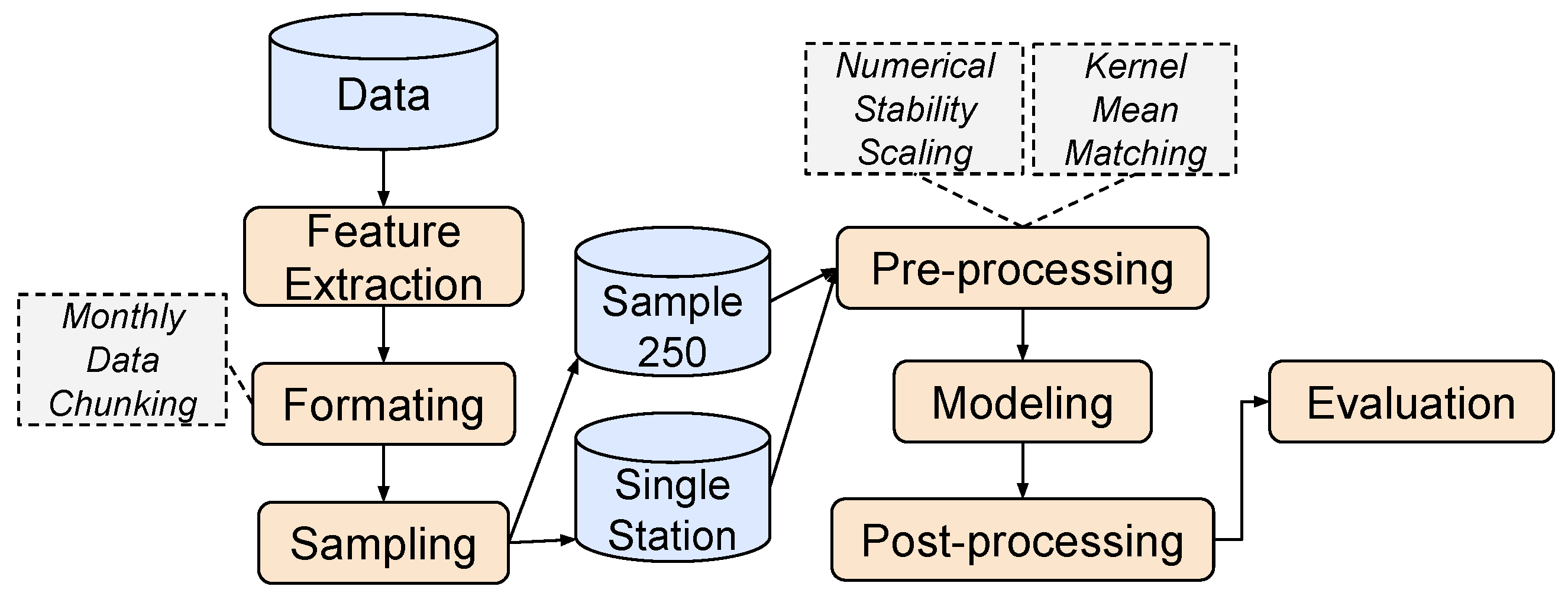
3.1. Choice of Covariates and Data Pre-Processing

We used the maximum daily temperatures recorded by stations in three regions in Japan (Tokyo, Osaka, and Kyushu) between 2003 and 2022 (see Figure 2). Tokyo and Osaka are major metropolitan areas whereas Kyushu is a southern island that is less developed and mountainous at the center. The 2003-2020 data were used as training dataset ${\mathcal{D}}_{\mathrm{train}}$, the 2021 data were used as validation dataset ${\mathcal{D}}_{\mathrm{valid}}$, and the 2022 data were used as test dataset ${\mathcal{D}}_{\mathrm{test}}$.

We set observation period $T\in \{1,2,\dots ,21\}$ differently in each experiment and set the non-observation period to $\tau =7$. Therefore, each data instance contained data for up to 28 days, including the observation period for inputs and the non-observation period for prediction, which depends on T. We only used the data on the first 28 days of each month and discarded the rest. The non-observation period was always from the 22nd to the 28th to ensure the same test data in all comparable scenarios. The observation period corresponded to the T days preceding the non-observation period. Data instances with missing values were excluded. Thus, the number of instances N in $\mathcal{D}$ was the number of years times 12 (months) times the number of stations minus the number of data instances with missing values. Our data preparation method ensures that no overlapping occurs among data instances, so our experimental DNN-based models cannot remember future data leaking through the inputs of other data instances. The data are summarized in

Table 1. Data statistics.

	Tokyo	Osaka	Kyushu
No. of data instances	14,869	11,678	20,095
No. of stations	75	59	102
Longitude	138.4–140.9	134.3–136.4	128.7–132.0
Latitude	34.9–37.2	33.4–35.8	27.4–34.7
Elevation (m)	2–1292	2–795	2–678
Average maximum temperature (°C)	19.2	19.9	21.5
Median maximum temperature (°C)	19.5	20.5	22.2

, and their mapping is shown in Figure 2.

The dataset contains the response variable of interest (maximum daily temperature) and several known covariates. More precisely, we used spatial information (longitude, latitude, and elevation of stations) and temporal information (recording dates) as predictors (Some predictors had large values, so we performed “numerical stability scaling” to avoid numerical overflow). The i-th sample for the t-th day was therefore composed of

• $z_{i,t}$: Maximum daily temperature;
• ${\xi }_{i,t}\left(1\right)$: Longitude;
• ${\xi }_{i,t}\left(2\right)$: Latitude;
• ${\xi }_{i,t}\left(3\right)$: Station elevation;
• ${\xi }_{i,t}\left(4\right)$: Record year;
• ${\xi }_{i,t}\left(5\right)$: Solar declination angle [17] estimated from recording date using

  $$\delta =23.{45}^{\circ }\times \sin ({360}^{\circ }\times \frac{\mathrm{nth}-\mathrm{day}-\mathrm{of}-\mathrm{the}-\mathrm{year}+284}{365});$$

  (19)
• ${\xi }_{i,t}\left(6\right)$: Solar noon angle = latitude − solar declination angle.

From Figure 3, we can see that, over the long term (Figure 3a), the patterns of the daily maximum temperatures among the three regions are similar (a pairwise correlation greater than 0.9), but when considering short periods, differences among regions emerge as shown in the monthly correlation analysis (Figure 3d). For example, in January 2022 (Figure 3b), the temperature range of Kyushu appears to differ greatly to Tokyo and Osaka: the Tokyo–Kyushu correlation is approximately 0.4 and the Tokyo–Osaka correlation is approximately 0.75. In July 2022 (Figure 3c), even though the temperature range appears to differ less between the Tokyo and Kyushu regions, the correlation analysis still shows that Tokyo and Kyushu differ even more, with their correlation being less than 0.4. Similar differences are also evident in several other months (Figure 3d). This is where we expect our system utilizing KMM to reduce the effect of the difference due to model training.

3.2. Model Settings

We created two low-resource data settings by sampling a small portion of the data in the target domain.

• Sample 250 data setting: We randomly sampled 250 instances from the full set of training data along with 50% (e.g., approximately 300 instances for Tokyo–Osaka) of the full set of validation data for the target domain. Thirty such samples were prepared.
• Single Station data setting: We separately evaluated each station in the target domain. In each single-station experiment, the target-domain train/validation/test datasets were for that station alone while the source-domain data were for all stations in the source-domain region.

The parameter settings for the proposed DNN-based domain adaptation model are as follows:

• High-dimensional representation size $n_h$: 32, 64, or 128.
• Number of layers in transformer encoder and transformer decoder modules: 2.
• Optimization algorithm: Adam [18] with a learning rate of 0.001, training with a batch size of 50, and a maximum of 1000 iterations.
• The best set of model parameters was selected using validation dataset ${\mathcal{D}}_{\mathrm{valid}}$.
• The RBF kernel coefficient in Equation (17) was $\gamma =0.1$.

Restriction on access to target-domain’s test data: While it appears productive to use the test inputs to estimate $\widehat{\beta }$ since the test inputs provide the most recent and potentially highest-quality information about the test data, it is impractical in our experimental settings. Therefore, we do not use any information from the test data to estimate $\widehat{\beta }$. Even if the inputs to the model are known for the test set, it is impractical to use all test instances in the application of KMM due to the temporal order; that is, we cannot use future data to estimate $\widehat{\beta }$ for past data instances. Moreover, in the single-station scenario, we can only access one test data instance at a time, which makes it impractical to apply KMM. In order to use the same KMM setting across all experiments, instead of the target-domain test data instances, we used the training and validation data, for which a more reasonable number of data instances is generally available.

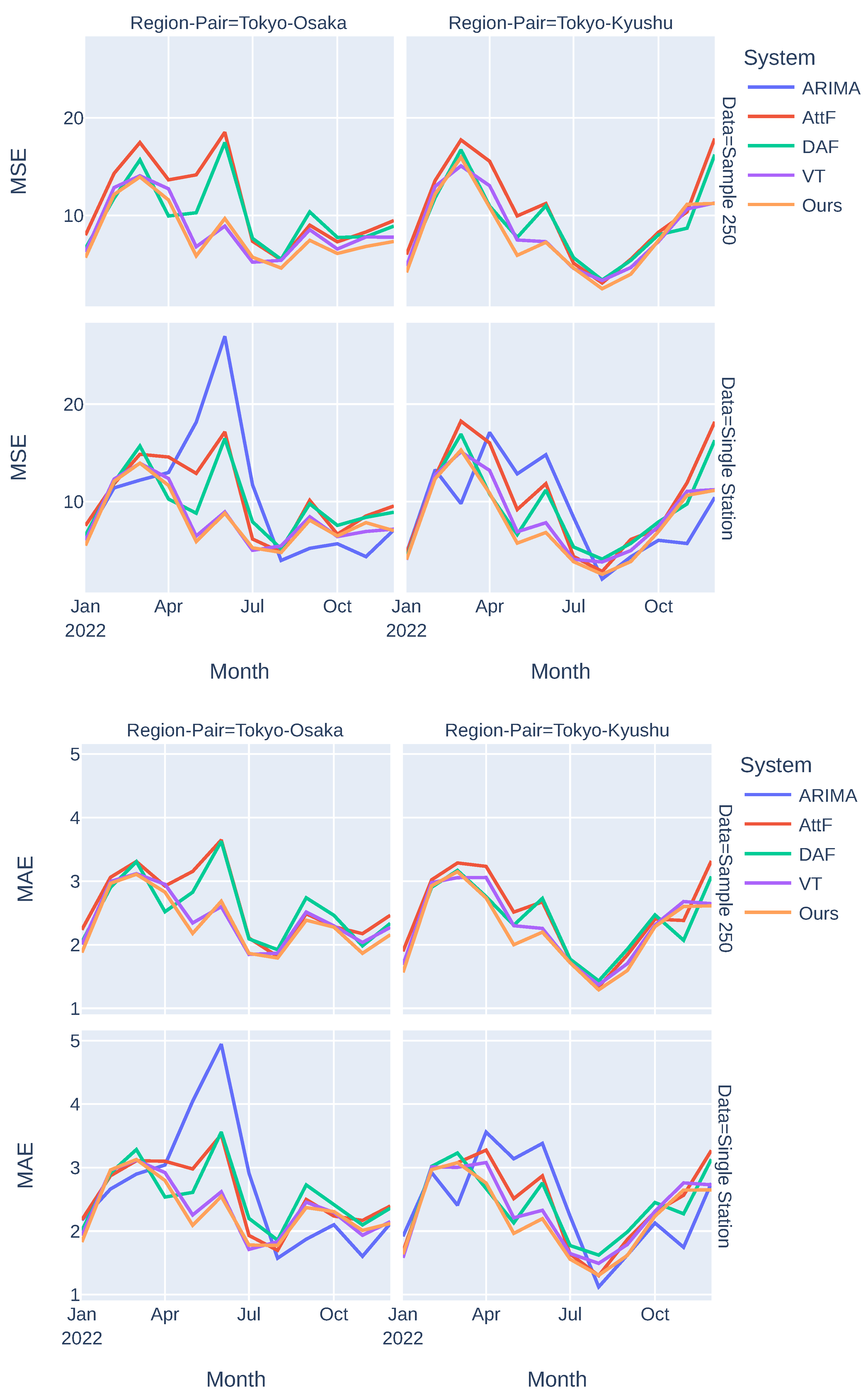
3.3. Evaluation

To assess the robustness of our DNN-based domain adaptation model, we compared and aggregated results for various sets of data settings, model hyper-parameters, parameter settings, and loss-function composition as follows:

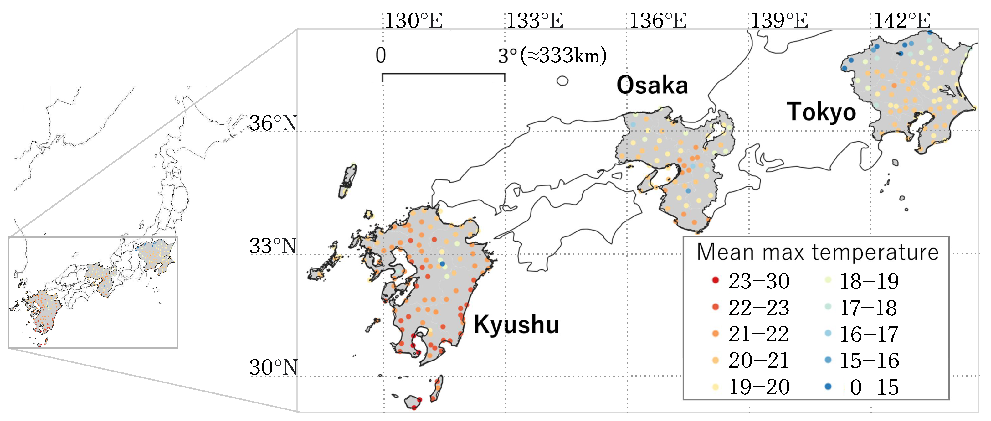
• Domain: Two source–target-domain pairs were considered: Tokyo–Osaka and Tokyo–Kyushu.
• Data: Two low-resource data settings (Sample 250 and Single Station) were used.
• Model: Three values of a high-dimensional representation size ($n_h\in \{32,64,128\}$) were used. The evaluation results reported later are the averaged evaluation metric values of all models with all three different representation sizes.
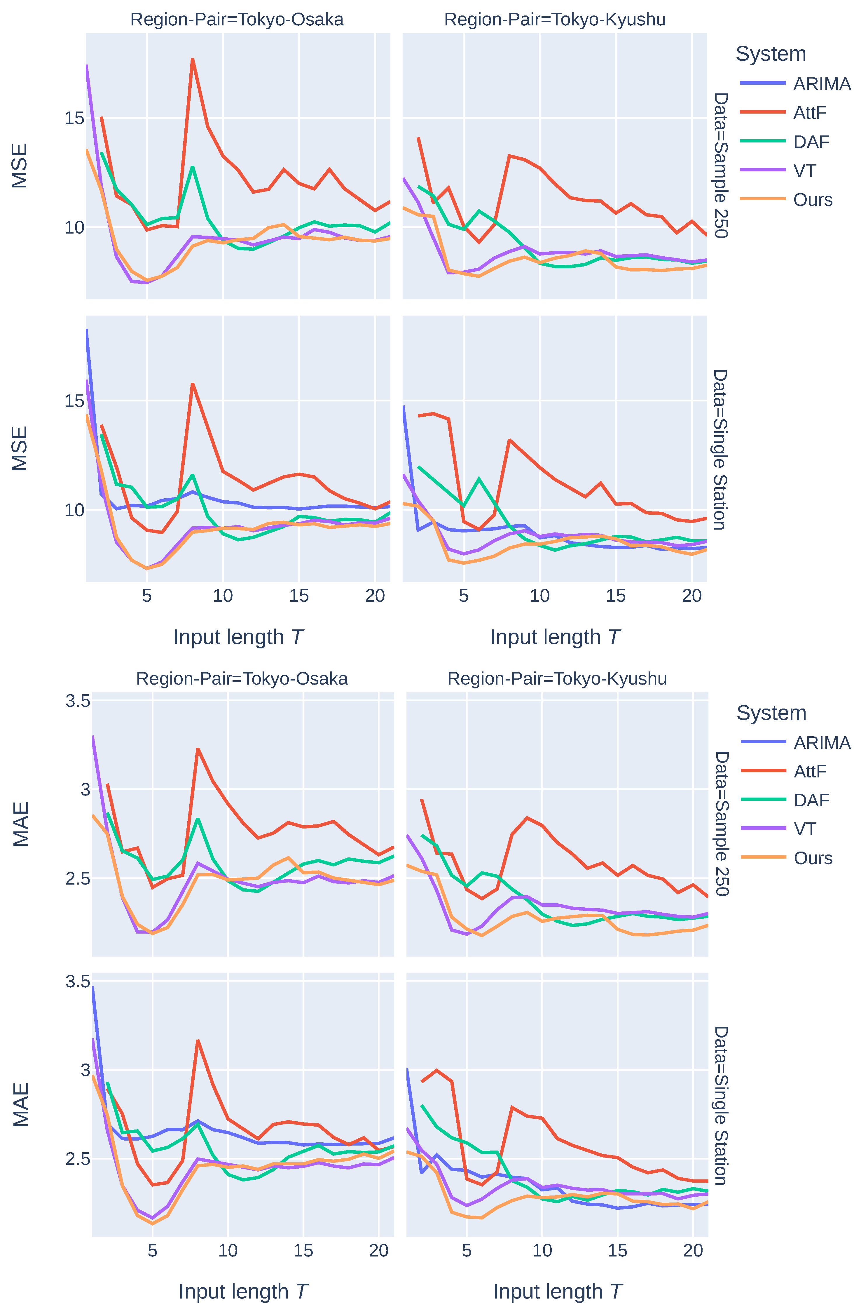
• Input Length $T\in \{1,2,\dots ,21\}$: $T=7$ was used as the representative input length for comparing our system with three baseline systems; the version of our system with the best performance was analyzed for different input lengths.
• Loss:

  –

  Domain weighting: Three values of $\alpha \in \{0,0.5,1\}$ were used for Equation (15).

  –

  KMM: KMM was both used and not used. $\widehat{\beta }$ in Equation (18) was set, respectively, by solving Equation (16) when using KMM or manually setting $\widehat{\beta }=1$ when not using KMM.

• Baseline systems:

  –

  VT: Our (vanilla) transformer-based architecture in a non-domain adaptation setting, which is equivalent to setting $\alpha =1$.

  –

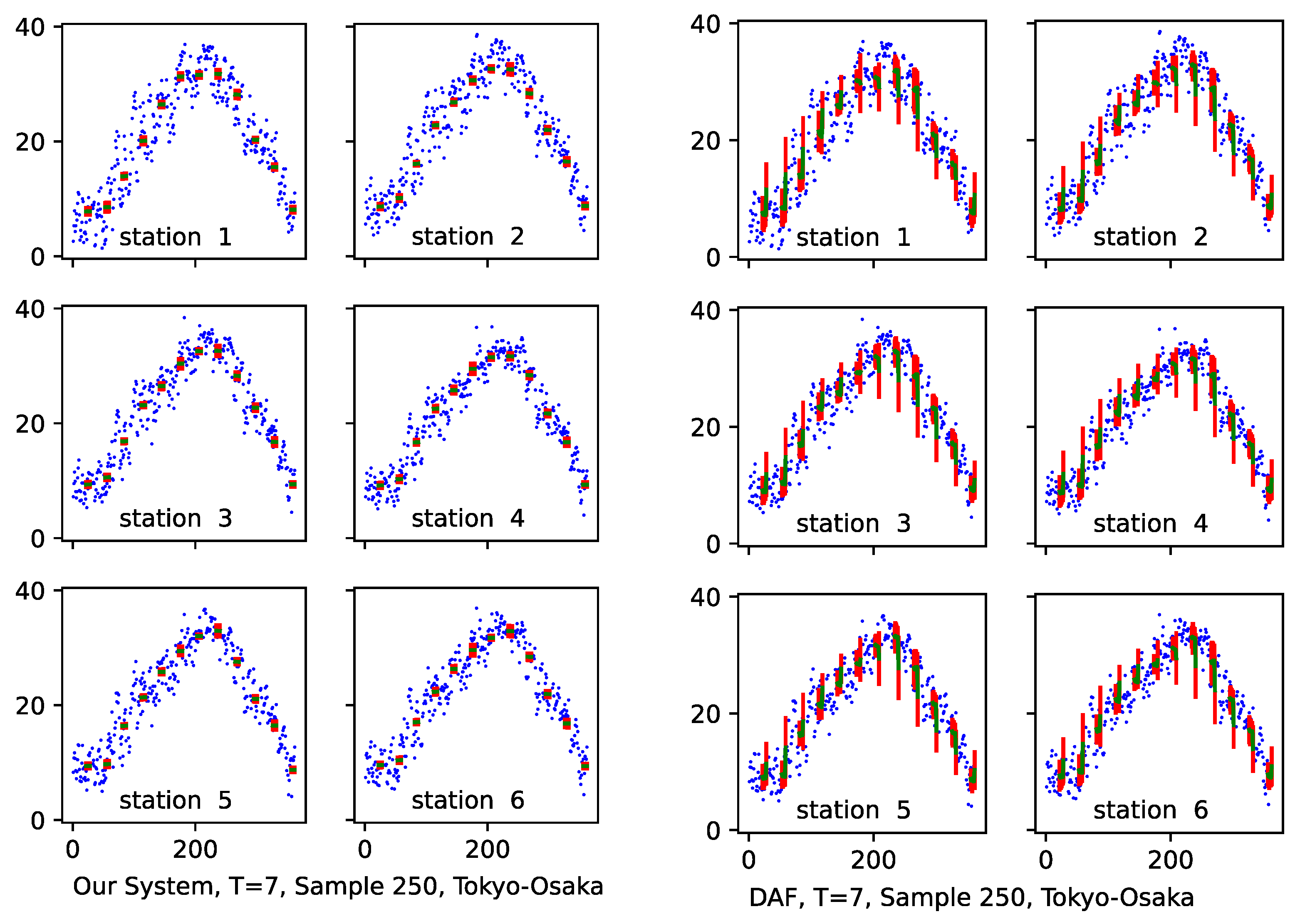
  DAF [11]: An advanced domain adaptation method for time-series forecasting that uses attention sharing in combination with domain discrimination. It was not evaluated for this particular temperature forecasting problem.

  –

  AttF [11]: The non-domain adaptation part of DAF (i.e., without shared attention and domain discrimination) and trained on only the target-domain data.

  –

  ARIMA [19]: A commonly used baseline for time-series forecasting in non-domain adaptation settings. The parameters were obtained using the same training data as those for the other evaluated systems.

Evaluation metrics: We used two evaluation metrics: the mean squared error (MSE) and mean absolute error (MAE). The Wilcoxon signed-rank test [20] was used to assess the significance of the results.

3.4. Results and Discussion

Effectiveness of domain adaptation: As shown in

Table 2. Evaluation results for the baseline systems and our original proposed system with $T=7$ (‘-’ means ‘not applicable’ and ‘bold’ means best value).

Evaluation Metric: MSE
	Sample 250	Sample 250	Single Station	Single Station
System	Tokyo–Osaka	Tokyo–Kyushu	Tokyo–Osaka	Tokyo–Kyushu
ARIMA	-	-	10.51	9.13
AttF	10.02	10.10	9.92	9.75
DAF	10.43	10.28	10.49	10.32
Ours, $\alpha$ = 1 (VT)	8.66	8.58	8.40	8.58
Ours, $\alpha$ = 0.5	8.46	8.28	8.16	8.16
Ours, $\alpha$ = 0	8.22	8.36	8.22	8.15
Ours, $\alpha$ = 0.5 & KMM	8.38	8.37	8.14	8.16
Ours, $\alpha$ = 0 & KMM	8.15	8.11	8.19	7.87
Evaluation Metric: MAE
	Sample 250	Sample 250	Single Station	Single Station
System	Tokyo–Osaka	Tokyo–Kyushu	Tokyo–Osaka	Tokyo–Kyushu
ARIMA	-	-	2.66	2.41
AttF	2.52	2.44	2.49	2.42
DAF	2.60	2.51	2.61	2.54
Ours, $\alpha$ = 1 (VT)	2.42	2.32	2.37	2.33
Ours, $\alpha$ = 0.5	2.34	2.29	2.33	2.26
Ours, $\alpha$ = 0	2.33	2.30	2.34	2.25
Ours, $\alpha$ = 0.5 & KMM	2.35	2.29	2.31	2.28
Ours, $\alpha$ = 0 & KMM	2.35	2.23	2.33	2.22

, domain adaptation yielded significantly better performance (p-value < 0.001) in terms of both MSE and MAE for all four sets of experiments {Sample 250, Single Station} × {Tokyo–Osaka, Tokyo–Kyushu}. This indicates that domain adaptation is feasible and promising for daily maximum temperature forecasting for regions for which there are small amounts of data and that have characteristics different from those of regions for which there are abundant data. In addition, our proposed architecture yields a better performance than the baseline systems even in the most basic setting of exclusively using the small target-domain data for training. Furthermore, with domain adaptation, we can further boost our prediction performance.

Effect of applying KMM: As shown in Table 2, the application of KMM yielded the best performance for three out of four sets of experiments {Sample 250, Single Station} × {Tokyo–Osaka, Tokyo–Kyushu}. The observed results are significant. For Tokyo–Kyushu, the p-values are <0.001 for both MSE and MAE. For Tokyo–Osaka, in terms of MSE, the p-values are <0.001 and 0.022, respectively, for the Sample 250 and Single Station data settings. For Tokyo–Osaka, in terms of MAE, the performance of applying KMM is better for the Single Station data setting but worse for the Sample 250 data setting, both with p-values of <0.001. Recalling that KMM is aimed at mitigating the domain difference between the source and target domains, the significance test shows that KMM is effective in improving temperature forecasting performance. This suggests that KMM should be effective in mitigating the difference between the source and target domains.

As shown in Figure 4, in an analysis of monthly prediction performance for all four sets of experiments, our domain adaptation approach ($\alpha$ = 0 & KMM ) consistently performs the best or competitively in the majority of situations in different seasons. In particular, our approach performs relatively more effectively than other approaches, e.g., ARIMA, AttF, and DAF, from May to July in the seasonal transition from cold to hot.

As shown in Figure 5, given different sets of training data over the 30 random samples in the Sample 250 data settings, our approach ($\alpha$ = 0 & KMM) to mitigating the domain difference by using KMM yields more stable predictions than DAF, which resolves domain difference by using domain discrimination. This is because our system with “$\alpha$ = 0 & KMM” adjusts the source-domain sample weights gradually and is not directly or greatly affected by the randomly sampled target-domain data, which direct affect DAF’s training mechanism.

Performance with different high-dimensional representation sizes: As shown in

Table 3. Evaluation results of our original proposed system with “$\alpha$ = 0 & KMM”, $T=7$, and different values of our high-dimensional model representation sizes (‘bold’ means best value). The models with representation sizes of 32 and 64 perform better than those with a representation size of 128.

Evaluation Metric: MSE
	Sample 250	Sample 250	Single Station	Single Station
System	Tokyo–Osaka	Tokyo–Kyushu	Tokyo–Osaka	Tokyo–Kyushu
32	8.25	7.85	8.18	7.67
64	7.79	8.00	8.09	7.82
128	8.40	8.49	8.29	8.12
Evaluation Metric: MAE
	Sample 250	Sample 250	Single Station	Single Station
System	Tokyo–Osaka	Tokyo–Kyushu	Tokyo–Osaka	Tokyo–Kyushu
32	2.36	2.20	2.31	2.21
64	2.34	2.20	2.31	2.23
128	2.36	2.28	2.35	2.24

, for our approach ($\alpha$ = 0 & KMM), the models with representation sizes of 32 and 64 perform better than those with a representation size of 128, though the differences are minimal in many cases. In addition, the models with a representation size of 128 still perform better than the non-adaptation models, whose results (shown in Table 2) are averaged over three representation sizes.

Bias in small target-domain training data: The additional use of source-domain data is more effective than the exclusive use of a small amount of target-domain training data. As shown in Table 2, exclusive training with small target-domain data without source-domain training data did not yield good performance. One reason for this is that the model is overfitted with bias patterns when only a small amount of target-domain data are exclusively used for training. When presenting with additional data from the source-domain, we start to observe an improvement in the prediction performance. Even with an $\alpha$ value of 0.5 equalizing the contribution of the small amount of target-domain training data and the larger amount of source-domain training data, we can still observe improvement. For $\alpha =0$ and KMM, even though a small amount of target-domain training data were used by KMM to estimate source-domain data weights $\widehat{\beta }$, the loss was optimized in accordance with the patterns in the source-domain data and not with those in the target-domain training data, which prevented direct learning of the bias patterns.

Effect of input length: As shown in Figure 6, our system achieved the best performance with input length $T\in \{5,6\}$. The performance worsened as the input length increased. This could be due to the increasing input length also increasing the complexity of inputs when the number of data samples is limited by the increasing number of model weights needed to learn more input data. Additionally, this could be because our system is based on the transformer DNN, which is a more complex neural network architecture, making it more susceptible to overfitting than, for instance, ARIMA or DAF, which use a convolutional neural network [21]. Compared with ARIMA and DAF, our system achieved a considerably better performance when the input length was small ($T<10$) and a similar performance when it was larger ($T\ge 10$). In other words, our system is also advantageous when there is a limited amount of input data. Notably, our system when using small values of $T\in \{5,6\}$ performed better than DAF at its best with $T=12$.

In cases where there is access to more historical data or a longer input length, it is possible to consider long-term analysis techniques, including (auto-)correlation and seasonal trend analyses, which are incorporated into Autoformer [22], a transformer-based architecture that replaces attention with auto-correlation for long-term time-series forecasting. We conducted a preliminary experiment of our domain adaptation approach by replacing our simpler transformer model with Autoformer. The preliminary experiment showed that its performance increases with the input length. However, with short input lengths as in our experiments, it did not achieve a better performance than simply using the transformer model with its original attention mechanism. For example, the MSE with Autoformer for Tokyo–Osaka × Sample 250 was 9.4 (vs. 8.15 with our system) and, for Tokyo–Kyushu × Sample 250, it was 8.8 (vs. 8.11 with our system).

Small prediction variances: We observed that our system’s predictions had small variances for each 7-day period. As shown in Figure 5, the daily maximum temperature frequently fluctuated with a high variance. We suspect that, given the lack of information due to the limitations in our settings, our system attempted to avoid overfitting to the high-frequency fluctuation during training by learning to predict the average values. One method for preventing this is to separate the predictions for each day in a seven-day period by modifying the transformer inputs:

$$h_{1:T}^{en{c}^{\prime }}=\mathrm{Transformer}-\mathrm{Encoder}\left(\mathrm{Projection}\left({\left\{z_{i,t}\right\}}_{t=1}^T,{\left\{{\xi }_{i,t}\right\}}_{t=1}^T;{\theta }_{a^{\prime }}\right);{\theta }_{e^{\prime }}\right)$$

(20)

$$h_{T+j}^{de{c}^{\prime }}=\mathrm{Transformer}-\mathrm{Decoder}(h_{T+1:T+j}^{\prime },h_{1:T}^{en{c}^{\prime }};{\theta }_{d^{\prime }}):j\in \{1,\dots ,\tau \},$$

(21)

where

$$h_{T+1:T+j}^{\prime }=\mathrm{Projection}\left(z_{i,T},{\left\{{\widehat{z}}_{i,t}\right\}}_{t=T+1}^{T+j-1},{\left\{{\xi }_{i,t}\right\}}_{t=T+1}^{T+j};{\theta }_{a^{\prime }}\right)$$

(22)

and by enforcing the prediction of the trend by substituting the predicted values ${\left\{{\widehat{z}}_t\right\}}_{t=T+1}^{T+j-1}$ with ${\left\{z_t\right\}}_{t=T+1}^{T+j-1}$ for Equation (22) during training. During prediction, previously predicted values ${\left\{{\widehat{z}}_t\right\}}_{t=T+1}^{T+t}$ are used for recursively predicting the next time step value ${\widehat{z}}_{T+t+1}$. In a preliminary experiment (

Table 4. Evaluation results for our original proposed system and its modified system when predictions for each day in a seven-day period were separated with $T=7$. The evaluation metric is MSE. ‘Bold’ means best value.

	Sample 250	Sample 250	Single Station	Single Station
System	Tokyo–Osaka	Tokyo–Kyushu	Tokyo–Osaka	Tokyo–Kyushu
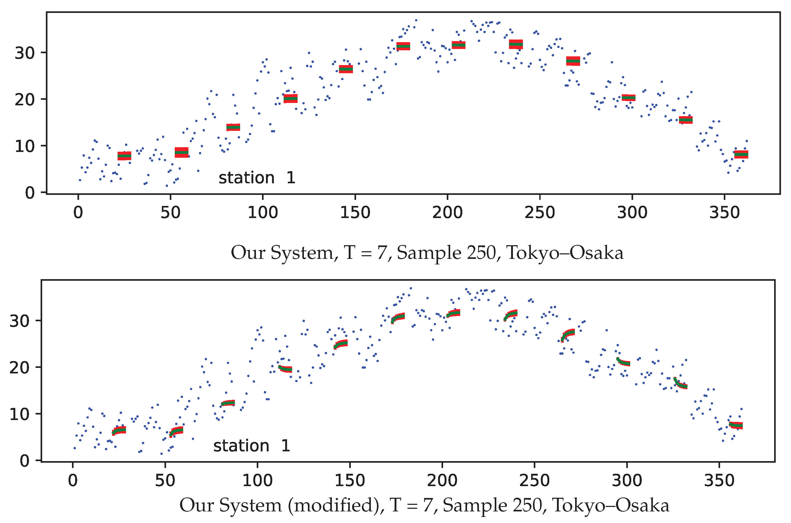
Ours, $\alpha$ = 0 & KMM	8.15	8.11	8.19	7.87
Ours, $\alpha$ = 0 & KMM, modified	9.66	7.94	9.75	8.42

), we analyzed such a system and observed that it tried to make fluctuating predictions (as shown in Figure 7) but yielded a worse performance than the system predicting average values.

Need for additional parameters: In this study, we only considered a scenario in which we have access to a very limited amount of data (recorded temperatures) and already known spatial–temporal information along with the derivable sun-declination angle. There are, however, several other parameters that greatly affect temperature. As shown above, given a limited input for a limited time span, attempting to predict short-term trends results in poor performance, i.e., it is challenging to capture and predict short-term trends. Future studies thus include expanding the number of parameters; including other types of weather data, e.g., rainfall, wind speed, and sunlight hours, as well as satellite data; and using a sophisticated framework that can perform domain adaptation across multiple covariates. However, the complexity of such a framework is drastically increased since it is much more difficult to assess the domain differences when there is more than one parameter. Such a framework with a complicated system of dependency differs from our approach in this study, which is to assess domain differences straightforwardly with a single parameter of interest, i.e., the daily maximum temperature. A further limitation of our current study is the use of only one year of data for validation (2021) and testing (2022). Unique weather patterns in these years (e.g., an unusual heatwave or cold spell) could have impacted the model tuning, or might have resulted in a higher test error than could be expected in a more typical year. Future studies, therefore, need to address the risk of unique weather patterns caused by such unusual weather-related events by, for example, including these events as potential parameters.

4. Conclusions

The research undertaken in this study illuminates the potential and challenges of using deep neural networks (DNNs), specifically transformer DNNs, for domain adaptation in daily maximum temperature forecasting, particularly in regions lacking sufficient data and supporting covariates.

The experimental results affirm the effectiveness of domain adaptation techniques, especially when applied to geographical areas for which there are small amounts of data and that exhibit characteristics dissimilar from regions for which there are abundant data. Application of our domain adaptation strategy resulted in significant performance improvements as demonstrated by two metrics: the mean squared error and mean absolute error. Furthermore, kernel mean matching (KMM) was shown to be a potent tool, facilitating performance enhancement for a majority of the experimental settings. KMM effectively helped in bridging the domain differences between the source and target regions, thus underscoring its potential utility in forecasting tasks across different geographical regions.

As we observed that domain adaptation is more effective than training exclusively on a small amount of target-domain training data, we can mitigate model overfitting to bias patterns inherent in the small amount of training data by leveraging additional data from a different source domain. We also observed that the effect of input length varies for each source–target pair, possibly due to the differences among regions. This suggests the need for future studies to expand domain adaptation to take this into account. Furthermore, we observed that a short-term trend is difficult to capture with short-term inputs, so it is necessary to investigate domain adaptation with additional parameters that affect temperature; for instance, wind speed and rainfall. However, it should be noted that the complexity of a system with more parameters could make utilizing domain adaptation much more challenging than what was approached in this study.

In summary, this study advances our understanding of the practical application of DNNs in temperature forecasting, particularly for regions that lack ample data. While the results reinforce the benefits of domain adaptation with the utility of KMM, they also point to the need for careful consideration when using target-domain data to avoid model overfitting. The results also underscore the importance of tailoring the input length to specific source–target pairs for optimal forecasting performance. Future research should delve deeper into methods for avoiding overfitting while harnessing target-domain data and should further investigate how different factors, such as input length, affect model performance across various geographical regions.

References

- Lee, S.; Lee, Y.S.; Son, Y. Forecasting daily temperatures with different time interval data using deep neural networks. Appl. Sci. 2020, 10, 1609. [Google Scholar] [CrossRef]
- Jasiński, T. Use of new variables based on air temperature for forecasting day-ahead spot electricity prices using deep neural networks: A new approach. Energy 2020, 213, 118784. [Google Scholar] [CrossRef]
- Rasp, S.; Lerch, S. Neural networks for postprocessing ensemble weather forecasts. Mon. Weather. Rev. 2018, 146, 3885–3900. [Google Scholar] [CrossRef]
- Vaswani, A.; Shazeer, N.; Parmar, N.; Uszkoreit, J.; Jones, L.; Gomez, A.N.; Kaiser, Ł.; Polosukhin, I. Attention is all you need. In Proceedings of the Advances in Neural Information Processing Systems, Long Beach, CA, USA, 4–9 December 2017; Volume 30.
- Zhao, W.X.; Zhou, K.; Li, J.; Tang, T.; Wang, X.; Hou, Y.; Min, Y.; Zhang, B.; Zhang, J.; Dong, Z.; et al. A survey of large language models. arXiv 2023, arXiv:2303.18223. [Google Scholar]
- Crabtree, C.J.; Zappalá, D.; Hogg, S.I. Wind energy: UK experiences and offshore operational challenges. Proc. Inst. Mech. Eng. Part A J. Power Energy 2015, 229, 727–746. [Google Scholar] [CrossRef]
- Sun, Q.; Yang, L. From independence to interconnection—A review of AI technology applied in energy systems. CSEE J. Power Energy Syst. 2019, 5, 21–34. [Google Scholar]
- Zhou, G.; Xie, Z.; Huang, X.; He, T. Bi-transferring deep neural networks for domain adaptation. In Proceedings of the 54th Annual Meeting of the Association for Computational Linguistics (Volume 1: Long Papers), Berlin, Germany, 7–12 August 2016; pp. 322–332. [Google Scholar]
- Singhal, P.; Walambe, R.; Ramanna, S.; Kotecha, K. Domain Adaptation: Challenges, Methods, Datasets, and Applications. IEEE Access 2023, 11, 6973–7020. [Google Scholar] [CrossRef]
- Cifuentes, J.; Marulanda, G.; Bello, A.; Reneses, J. Air temperature forecasting using machine learning techniques: A review. Energies 2020, 13, 4215. [Google Scholar] [CrossRef]
- Jin, X.; Park, Y.; Maddix, D.; Wang, H.; Wang, Y. Domain adaptation for time series forecasting via attention sharing. In Proceedings of the International Conference on Machine Learning, PMLR, Baltimore, MD, USA, 17–23 July 2022; pp. 10280–10297. [Google Scholar]
- Bernstein, A.S.; Sun, S.; Weinberger, K.R.; Spangler, K.R.; Sheffield, P.E.; Wellenius, G.A. Warm season and emergency department visits to US Children’s Hospitals. Environ. Health Perspect. 2022, 130, 017001. [Google Scholar] [CrossRef] [PubMed]
- Nakamura, S.; Kusaka, H.; Sato, R.; Sato, T. Heatstroke risk projection in Japan under current and near future climates. J. Meteorol. Soc. Japan Ser. II 2022, 100, 597–615. [Google Scholar] [CrossRef]
- Ba, J.L.; Kiros, J.R.; Hinton, G.E. Layer normalization. arXiv 2016, arXiv:1607.06450. [Google Scholar]
- Hendrycks, D.; Gimpel, K. Gaussian error linear units (gelus). arXiv 2016, arXiv:1606.08415. [Google Scholar]
- Huang, J.; Gretton, A.; Borgwardt, K.; Schölkopf, B.; Smola, A. Correcting sample selection bias by unlabeled data. In Proceedings of the Advances in Neural Information Processing Systems, Vancouver, BC, Canada, 4–9 December 2006; Volume 19. [Google Scholar]
- Iqbal, M. An Introduction to Solar Radiation; Elsevier: Amsterdam, The Netherlands, 2012. [Google Scholar]
- Kingma, D.P.; Ba, J. Adam: A method for stochastic optimization. arXiv 2014, arXiv:1412.6980. [Google Scholar]
- Shumway, R.H.; Stoffer, D.S.; Shumway, R.H.; Stoffer, D.S. ARIMA models. In Time Series Analysis and Its Applications: With R Examples; Springer: Berlin/Heidelberg, Germany, 2017; pp. 75–163. [Google Scholar]
- Conover, W.J. Practical Nonparametric Statistics; John Wiley & Sons: Hoboken, NJ, USA, 1999; Volume 350. [Google Scholar]
- Albawi, S.; Mohammed, T.A.; Al-Zawi, S. Understanding of a convolutional neural network. In Proceedings of the 2017 international conference on engineering and technology (ICET), Antalya, Turkey, 21–23 August 2017; IEEE: Piscataway, NJ, USA, 2017; pp. 1–6. [Google Scholar]
- Wu, H.; Xu, J.; Wang, J.; Long, M. Autoformer: Decomposition transformers with auto-correlation for long-term series forecasting. In Proceedings of the Advances in Neural Information Processing Systems, Virtual, 6–14 December 2021; Volume 34, pp. 22419–22430. [Google Scholar]