Abstract
Noctilucent clouds (NLC) are sensitive indicators in the upper mesosphere, reflecting changes in the background atmosphere. Studying NLC responses to the solar cycle is important for understanding solar-induced changes and assessing long-term climate trends in the upper mesosphere. Additionally, it enhances our understanding of how increases in greenhouse gas concentration in the atmosphere impact the Earth’s upper mesosphere and climate. This study presents long-term trends in the response of NLC and the background atmosphere to the 11-year solar cycle variations. We utilised model simulations from the Leibniz Institute Middle Atmosphere (LIMA) and the Mesospheric Ice Microphysics and Transport (MIMAS) over 170 years (1849 to 2019), covering 15 solar cycles. Background temperature and water vapour (H2O) exhibit an apparent response to the solar cycle, with an enhancement post-1960, followed by an acceleration of greenhouse gas concentrations. NLC properties, such as maximum brightness (βmax), calculated as the maximum backscatter coefficient, altitude of βmax (referred to as NLC altitude) and ice water content (IWC), show responses to solar cycle variations that increase over time. This increase is primarily due to an increase in background water vapour concentration caused by an increase in methane (CH4). The NLC altitude positively responds to the solar cycle mainly due to solar cycle-induced temperature changes. The response of NLC properties to the solar cycle varies with latitude, with most NLC properties showing larger and similar responses at higher latitudes (69° N and 78° N) than mid-latitudes (58° N).
1. Introduction
Noctilucent clouds (NLC), consisting of tiny ice particles, form about 80–85 km above the Earth’s surface and are the highest atmospheric clouds. These clouds typically form in the summer when temperatures in the mesopause region are very low, especially at middle and polar latitudes [1,2]. NLC are rare, having only been observed in modern times since the end of the 19th century [3]. By studying NLC, we can gain insight into changes in the upper mesosphere and their potential implications for climate research [4,5,6,7,8,9]. The formation of NLC is a complex process that depends on several factors, including background temperature and water vapour [6,10]. When the temperature in the mesosphere falls below the freezing point of water (~150 K), water vapour can condense and form ice particles, which are the building blocks of NLC. In general, the combination of low background temperatures and sufficient water vapour concentrations creates favourable conditions for forming NLC [1,3,4].
The 11-year solar cycle is one of the factors that can influence mesospheric temperature and water vapour and thereby affect the formation and properties of NLC [11,12]. It is important to understand how the solar cycle relates to the characteristics of NLC to study how they behave and affect the upper atmosphere. Numerous studies have been conducted on the relationship between the 11-year solar cycle and the properties of NLC (e.g., [8,13,14,15,16]). Satellite observations and model simulations are used to investigate the effects of the solar cycle on the background atmosphere and their impacts on NLC properties. A positive correlation exists between the solar Lyman-alpha (Lyα) flux and the background temperature at NLC altitudes. Depending on the altitude, the correlation can be positive or negative for water vapour [17]. Studies have shown a clear anti-correlation between the solar cycle Lyα and ice water content (IWC) during solar cycles 22 and 23, but it decreases during the recent solar cycle 24 [13,17]. Our previous study [17] found a clear anti-correlation between Lyα flux and IWC in the model and satellite observations for solar cycles 22 and 23, which becomes weaker in solar cycle 24. Moreover, the magnitude of the solar cycle-induced IWC variations in Solar Backscatter Ultraviolet (SBUV) and Halogen Occultation Experiment (HALOE) satellite observations is the same as the IWC variations in the MIMAS model. The study showed that the reduced IWC response during solar cycle 24 is due to the reduced variation of Lyα during this particular solar cycle.
The observational data available for NLC trends are still quite limited, and little is known about long-term trends and episodic changes in the background atmosphere at NLC altitudes [7,9,11,18]. Therefore, there needs to be detailed studies or sufficient information on the long-term evolution of the solar cycle response of NLC. Model simulations are valuable tools to help us learn more about the changes in the NLC and the surrounding atmosphere [19]. Long-term simulations of NLC by the MIMAS model from 1849 to 2019 are promising for studying solar cycle trends (covering 15 complete solar cycles) in the NLC, as the model uses the solar Lyα flux as a proxy for solar irradiance [9,20]. Therefore, by using the MIMAS model, the response of NLC properties to the solar cycle, such as ice particle radius, IWC, the backscatter coefficient at a wavelength of 532 nm (β, from now on referred to NLC brightness) and NLC altitude, can be studied over a longer period, which is not possible with satellite observations due to measurement limitations. There are studies [9,20] using the MIMAS model regarding the long-term trends in NLC and the effects of increasing greenhouse gases (CO2 and CH4) from 1871 to 2008. The results show that some ice parameters’ time series significantly modulate with the solar cycle (see Figure 3 in [9]). Since those studies aimed to investigate long-term trends in NLC, the effects of solar cycle variation on NLC were excluded by averaging over half a solar cycle [20].
In this study, we mainly focus on the impact of the 11-year solar cycle variation on the properties of NLC during the period 1855–2019, relying on the model simulations used in previous studies [9,20]. Compared to previous studies, this study includes an analysis of long-term trends in the vertical distribution profiles of the background atmosphere, including temperature and water vapour with and without NLC. In addition, we examine trends in the vertical distributions of NLC properties that have not been explored before, such as the number and radius of ice particles and NLC brightness. This paper aims to address the following questions: (1) How do background temperature and water vapour respond to the solar cycle, and what are the trends in their solar cycle response? (2) What are the long-term trends in the vertical distribution of NLC properties? How do solar cycle modulations influence them? (3) Which NLC properties are influenced by the 11-year solar cycle, and how strongly are they influenced? (4) What influence does the long-term increase in greenhouse gases have on the response of NLC properties to the solar cycle? (5) Is the response of NLC properties to the solar cycle dependent on latitude, and how strong? The following section briefly discusses the models used in this study. Section 3 presents the results and discussion on the trends in the response of the background atmosphere and NLC properties to the solar cycle, as well as the trends in their response to the solar cycle under the influence of increasing greenhouse gases and for different latitudes. The summary of our findings is provided in Section 4.
2. Model Description
Here, we only provide a brief description of the model setup, as a comprehensive explanation of our modelling framework has already been discussed in detail in various publications [9,20,21,22,23]. The overall model framework combines two models, namely the Leibniz Institute Middle Atmosphere (LIMA) model and the Mesospheric Ice Microphysics and Transport (MIMAS) model. The basic idea of this modelling framework is to use LIMA to model the background atmosphere under Northern Hemisphere conditions and then use this background information in the MIMAS model to calculate the properties of NLC (see Figure 1 in [20]). LIMA and MIMAS use daily Lyα data from the LASP Interactive Solar Irradiance Data Center (LISIRD) as a representative measure of solar activity from 1961 to 2019 [24]. Before 1961, monthly sunspot numbers approximated Lyα values. In LIMA, variations in Lyα flux account for atmospheric temperature variations, while in MIMAS, changes in Lyα flux cause photolysis of H2O.
LIMA is a global model that covers the altitude range from 0 to 150 km and includes key processes such as radiation, chemistry and transport [12,22]. At lower altitudes (0–28 km), LIMA is nudged to the twentieth-century reanalysis data from NOAA-CIRES (National Oceanic and Atmospheric Administration–Cooperative Institute for Research in Environmental Sciences 20CR; [25]). In LIMA, the mixing ratios of ozone (28–65 km) and carbon dioxide (28–150 km) change, whereas all other trace gases are constant. We consider temporal and latitudinal fluctuations in the stratosphere and lower mesosphere for ozone from 1961 to 2008 [12,26]. Before 1961, stratospheric ozone was kept constant (according to 1961). The model’s carbon dioxide (CO2) concentration is based on a monthly average time series from 1961 to 2019 measured at Mauna Loa (19° N, 155° W). Before 1961, historical CO2 data from Antarctic ice cores were used [27]. In LIMA, the influence of small-scale internal gravity waves is accounted for by a non-linear spectral gravity wave parameterisation [28].
Climate change and the solar cycle most likely affect the atmospheric circulation pattern in the mesosphere, which might affect the background conditions and gravity waves (for example, [29]). Unfortunately, very little is known about the long-term effects of these changes on the dynamic, thermal and compositional characteristics of the summer mesopause region. Since considering these potential long-term impacts is highly speculative, we decided to use a specific dynamic scenario from the representative year 1976 for the entire period from 1849 to 2019. It is important to note that the conclusions from our study are not influenced by the choice of this specific year. Consequently, this study does not consider any potential influence of mean background winds and wave activity trends on NLC [9,17,20].
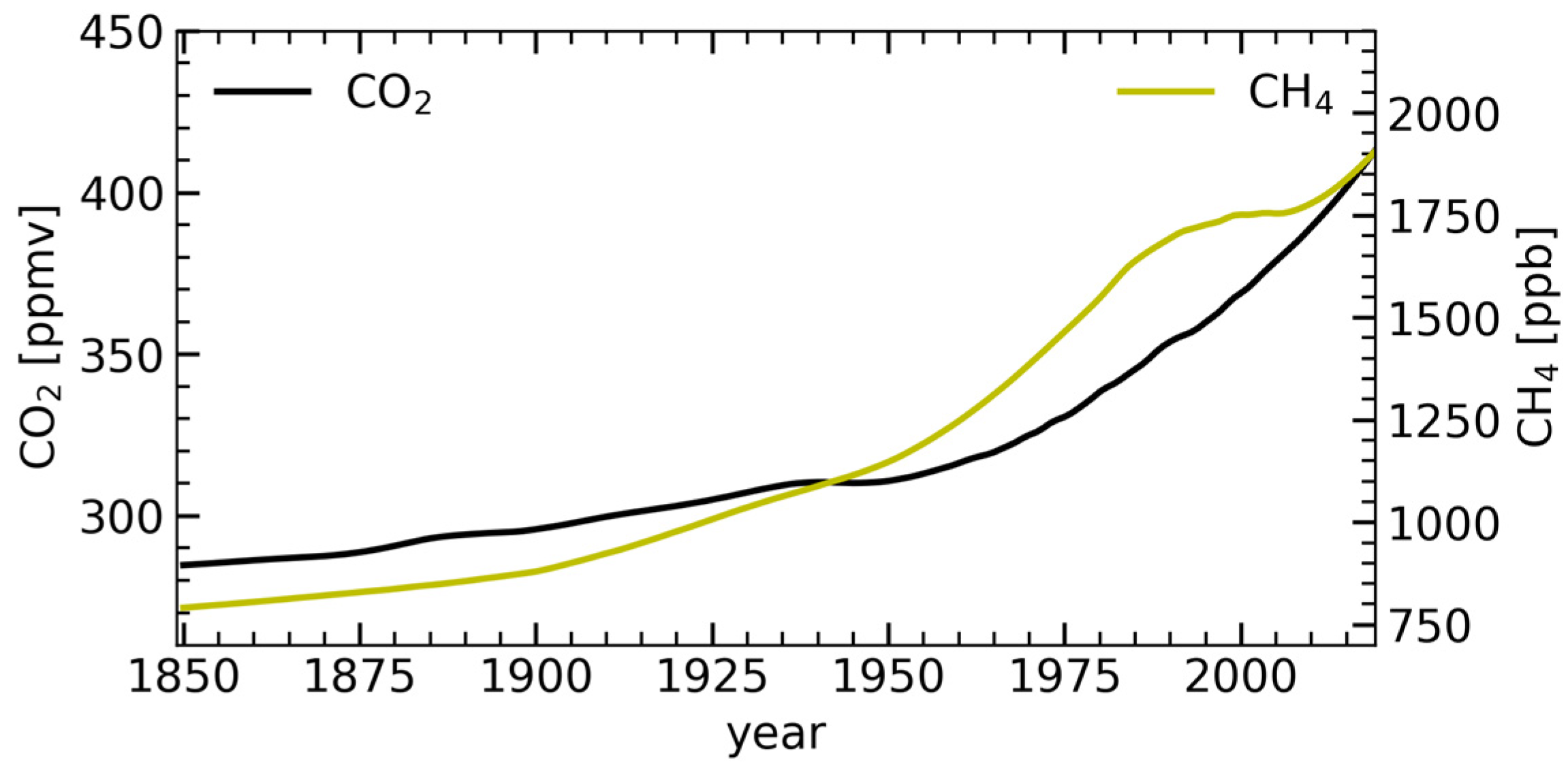
MIMAS is a specialised 3D Lagrangian transport model that simulates ice particles in the mesosphere and lower thermosphere (MLT) [9,17,20]. It calculates various NLC parameters from 10 May to 31 August and is restricted to mid and high latitudes (37°–90° N). The model uses a horizontal grid resolution of 1° in latitude and 3° in longitude, with a vertical resolution of 100 m, ranging from 77.8 to 94.1 km (163 levels). Below the lower boundary of MIMAS, two factors determine the mixing ratio of H2O in the stratosphere: first, the transport of H2O from the troposphere and second, the oxidation of methane (CH4), where each CH4 molecule produces two H2O molecules. Through photochemical processes, methane almost entirely converts into H2O in the mesosphere [9]. MIMAS assumes a constant transport rate from the troposphere. Therefore, the increase in H2O occurs mainly through methane oxidation. Therefore, we parameterise H2O as a function of CH4, following the approach proposed by [9]. Please note that H2O sources and sinks due to chemical reactions are not accounted for in MIMAS, which may lead to uncertainties in the model-calculated H2O concentrations. The time series of CH4 and CO2 used in the model simulations are shown in Figure 1. MIMAS contains about 40 million dust particles that can serve as condensation nuclei. These dust particles originate from meteors evaporating in the atmosphere (for more information, see [21,30]). Subsequently, these particles are coated with ice in regions where H2O is supersaturated and transported by three-dimensional and time-dependent background winds, eddy diffusion and sedimentation. Standard microphysical processes, including the Kelvin effect, determine the nucleation and growth of ice particles in MIMAS [4]. Please keep in mind that there are possible uncertainties regarding the number of dust particles available for condensation, as the accurate count of dust particles generated from evaporating meteorites is not available.

Figure 1.
Time series of CO2 and CH4 concentrations (1849–2019) used in model runs.
This study uses three model runs: A, B and C. In run A, we increase both CO2 and CH4 (H2O). In run B, only the CO2 concentration increases, while the CH4 concentration remains constant. In run C, the CH4 concentration increases while the CO2 concentration is constant. In this paper, the following symbols refer to these scenarios: CO2↑, CH4↑ for run A; CO2↑, CH4↔ for run B; and CO2↔, CH4↑ for run C. MIMAS output has a horizontal resolution of 120 longitude bands (0°–360°) and 53 latitude bands (each 1° from 38° N to 90° N). This study focuses on three latitudes in July: 58 ± 3° N (referred to as “mid”), 69 ± 3° N (referred to as “high”) and 78 ± 3° N (referred to as “arctic”).
3. Results and Discussion
3.1. Solar Cycle Effects on Background Temperature
We studied the impact of CO2 increases and solar cycle variations on the vertical distribution of temperatures for 1849–2019. The time series of the temperature profiles (Figure 2) shows that the profiles shift downwards over time.
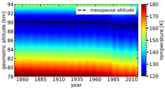
Figure 2.
Time series of temperature profiles zonally averaged at 69° N latitude for July as a function of geometric altitude.
This shift in profiles is due to atmospheric shrinking resulting from the cooling of the middle atmosphere by increasing CO2 [9,20]. Reference [9] examined the temperature trends for a fixed geometric altitude and a fixed pressure level (see Figure 1b in [9]). The temperature has decreased by 7 K since 1871 for a fixed altitude of 83 km but not significantly for a fixed pressure level. An increase in CO2 leads to a decrease in temperature in the stratosphere and lower mesosphere, mainly due to enhanced cooling by CO2 [12,23,31,32,33]. At NLC altitudes, this cooling leads to an altitude decrease in pressure levels because the atmosphere in the lower and middle mesosphere shrinks due to CO2 cooling, referred to as the “shrinking effect”. The negative temperature lapse rate at NLC altitudes causes the apparent cooling at geometric altitudes. The temperature decline at 83 km altitude accelerated after 1960, with the slope of the temperature trend line for the period 1960–2008 (m1) being ~6 times larger than the slope of the temperature trend line for the period 1871–1960 (m2), due to an accelerated CO2 increase. Temperature trends calculated by LIMA are consistent with observations near 45° N latitude in summer, with a cooling trend of 3 K/decade from 1979–1997 (see Figure 10 in [34] vs. Figure 1b in [23]).
The time series of the vertical temperature profiles clearly show the influence of the solar cycle on the background temperature at all altitudes and reveal distinct 11-year patterns in the profiles (Figure 2). During solar maximum, the increase in solar irradiance leads to greater absorption of solar radiation in the MLT region by molecular oxygen and water vapour, heating the background atmosphere. The temperature differences of 0.5 K–2 K observed between solar maximum and minimum at NLC altitudes depend on solar cycle intensity and altitude [17]. The temperature difference decreases at lower altitudes as the intensity of solar radiation decreases due to atmospheric absorption [17]. In summary, the results suggest that increasing CO2 and solar cycle variations significantly impact temperature profiles in the mesosphere and lower thermosphere.
3.2. Solar Cycle Effects on Background Water Vapour
The presence of water vapour in the upper atmosphere is mainly responsible for forming NLC. NLC are created when microscopic particles in the atmosphere, such as dust or debris, function as a surface for condensing water vapour. The saturation ratio of air with water vapour is defined as S = PH2O/Pice, where PH2O is the H2O partial pressure (CH2O* P), and Pice is the saturation vapour pressure over a plane ice surface (CH2O is the water vapour mixing ratio). An environment with value S > 1 is supersaturated, meaning ice particles can grow under these conditions, while S < 1 is subsaturated and leads to ice particle sublimation. The formation of NLC involves the removal of water vapour from the background atmosphere, known as the “freeze-drying effect”, and the release of H2O at altitudes where NLC sublimates. Regarding trends of water vapour in the middle atmosphere, there is no clear picture, even on decadal time scales [9,18]. There are few studies of water vapour trends in the mid-latitude summer mesopause region. Observations from the Solar Occultation For Ice Experiment (SOFIE) onboard NASA’s Aeronomy of Ice in the Mesosphere (AIM) satellite (Figure 6d in [35]) show that the H2O mixing ratio has been around four parts per million volume (ppmv) in recent years, which is in agreement with MIMAS as shown in Figure 1c (run A) in [9]. The recent study by [36] suggests a water vapour trend of about 5% per decade at 52.5° N and 80 km, corresponding to 0.175 ppmv per decade. This trend is consistent with trends calculated in MIMAS, which show a rate of 0.15 ppmv per decade (see Figure 1c in [9]). However, it is unfortunate that no information is available on the centennial evolution of temperatures or water vapour in the upper mesosphere [9].
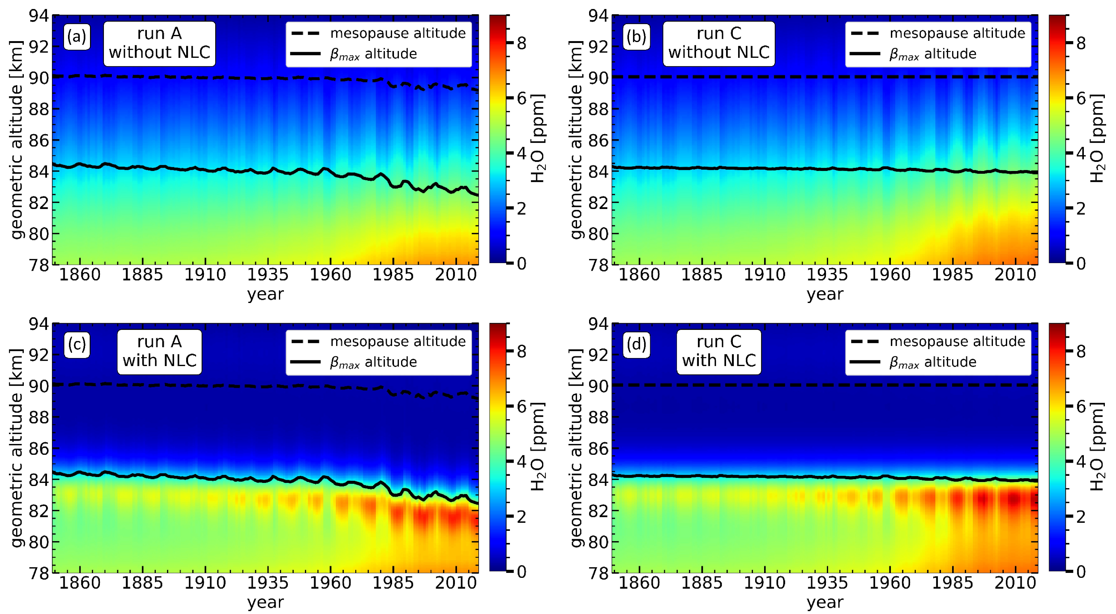
To investigate the effects of NLC formation on long-term water vapour trends, we conducted model simulations with and without NLC formation while keeping the same background conditions. The time series of the vertical water vapour distribution for MIMAS runs A and C (with and without NLC) are shown in Figure 3. Without NLC, the background H2O concentration increases with time at all altitudes in both run A and run C. At higher altitudes, more water vapour became available than at the beginning of the study period. This is due to increasing CH4, which leads to more H2O molecules forming during the oxidation of CH4. The H2O enhancement in run A is slightly lower than in run C for a given geometric altitude. This is due to the increasing CO2 concentration in run A, which causes atmospheric shrinking. Due to the negative H2O gradient with altitude, the downward shift in profile leads to a decrease in H2O concentration for a given geometric altitude. Consequently, for a fixed geometric altitude, the increase in H2O background due to CH4 oxidation is somewhat less pronounced in run A than in run C.
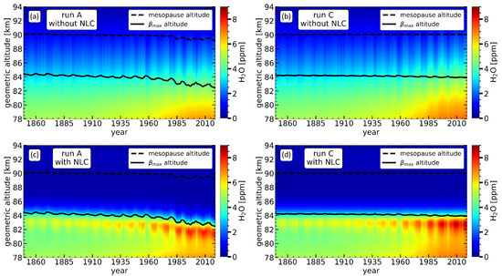
Figure 3.
Time series of water vapour concentration as a function of geometric altitude zonally (69° N) and monthly (July) averaged for (a) Run A without NLC, (b) Run C without NLC, (c) Run A with NLC and (d) Run C with NLC.
For H2O trends without NLC (Figure 3a,b), apparent effects of the solar cycle are observed in the form of maximum and minimum at 11-year intervals. During solar maximum, the water vapour concentration decreases at all altitudes due to an enhancement in photolysis caused by an increase in Lyα flux. For example, during solar cycle 23, the negative response reaches its maximum at approximately 87.5 km altitude [17]. Above this altitude, the impact of photolysis diminishes due to the decreasing mixing ratio of H2O, while below this altitude, the decrease is attributed to the decreasing intensity of solar Lyα radiation [17]. Comparing the figures with and without NLC (Figure 3, upper vs. lower plots), the H2O profile with NLC differs from that without NLC. At NLC formation altitudes (>~83–85 km), the H2O concentration decreases due to the removal of H2O during the formation of ice particles, a phenomenon known as the “freeze-drying effect”. As a result, the highest concentrations of H2O are found at the altitudes where NLC sublimation occurs, which is approximately 1 km below the βmax altitude (indicated by the solid black line). The enhancement in H2O concentration at the sublimation altitudes amplifies the response of H2O to the 11-year solar cycle at those altitudes. Moreover, in run A, the background H2O profiles exhibit a downward shift over time, attributed to the atmospheric shrinking caused by increasing concentration of CO2.
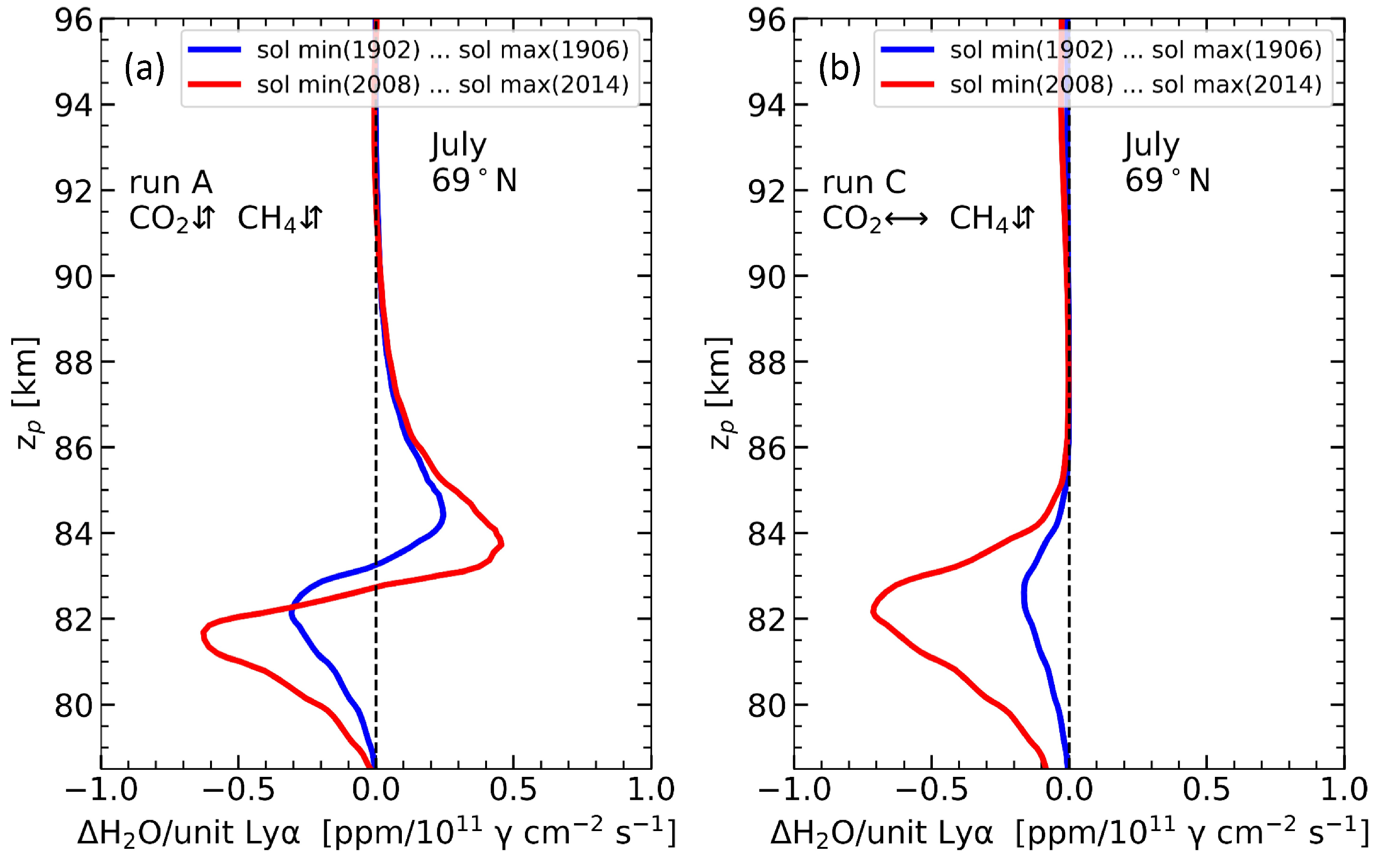
To investigate the long-term effects of increasing greenhouse gases on the solar cycle response of H2O, we calculated the H2O response profile with NLC for runs A and C. For this, first, we calculated the difference of H2O vertical profiles between solar maximum and minimum for two solar cycles, one at the beginning (1902–1906) and one at the end (2008–2014), which was then divided by the actual Lyα change between the solar maximum and minimum of the corresponding solar cycle. It provides us with the vertical profiles of water vapour response to a unit change in Lyα (i.e., absolute change in H2O for a unit Lyα change, hereafter called the H2O response profile). Figure 4 shows the H2O response profiles for runs A and C. In Figure 4a (run A), the H2O response profile shows positive and negative values depending on altitude. According to [17], the solar cycle affects the H2O concentration in the upper mesosphere mainly in two ways: directly through the photolysis and, at the time and place of NLC formation, indirectly through temperature changes. The photolysis effect leads to an anti-correlation between the H2O concentration and the solar Lyα, even more pronounced at altitudes below ~83 km where NLC ice particles sublimate. Above ~83 km, where NLC form, the H2O concentration correlates positively with solar cycle Lyα variations. The reason for this positive response is that during solar maximum, the background atmosphere becomes warmer due to higher solar activity, causing relatively less ice formation compared to solar minimum. The lower ice formation rate leads to less water vapour consumption from the background atmosphere, resulting in a relatively higher H2O concentration left in the background during solar maximum compared to solar minimum. For run C, there is no positive response of H2O due to the constant background temperature used for all years. Comparing early and late solar cycles in runs A and C shows that the magnitude of the H2O response profile has increased significantly in the later solar cycle. This increased response in run A is due to an increase of CO2 and CH4, i.e., an increase in CO2 leads to cooling of the background atmosphere, which leads to an intensification of the microphysical processes at ice formation altitudes and thus more effect on the magnitude of positive response. In addition, the increase in CH4 leads to more water vapour in the upper mesosphere, resulting in a higher background H2O concentration, which, in turn, leads to a larger effect of photolysis on H2O at NLC sublimation altitudes. In run C (Figure 4b), the magnitude of the negative response significantly increased during the late solar cycle, mainly due to H2O enhancement by CH4. Further details on the mechanism of the water vapour response to the solar cycle and the effects of increasing greenhouse gases are better described in [17].
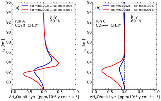
Figure 4.
H2O response per unit Lyα variations as a function of pressure altitude. (a) MIMAS run A with increasing CO2 and CH4; (b) MIMAS run C with increasing CH4 and constant CO2.
3.3. Trends in Vertical Profiles of NLC Properties
In this section, we investigate the long-term trends in NLC properties as a function of geometric altitude under different atmospheric greenhouse gas conditions (runs A, B and C). Figure 5 shows the time series of vertical profiles for the number, radius and brightness of ice particles. All these profiles are zonally and monthly averaged at latitudes 69 ± 3° N.
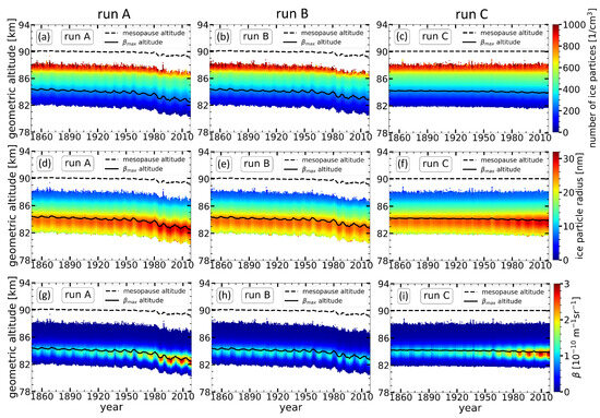
Figure 5.
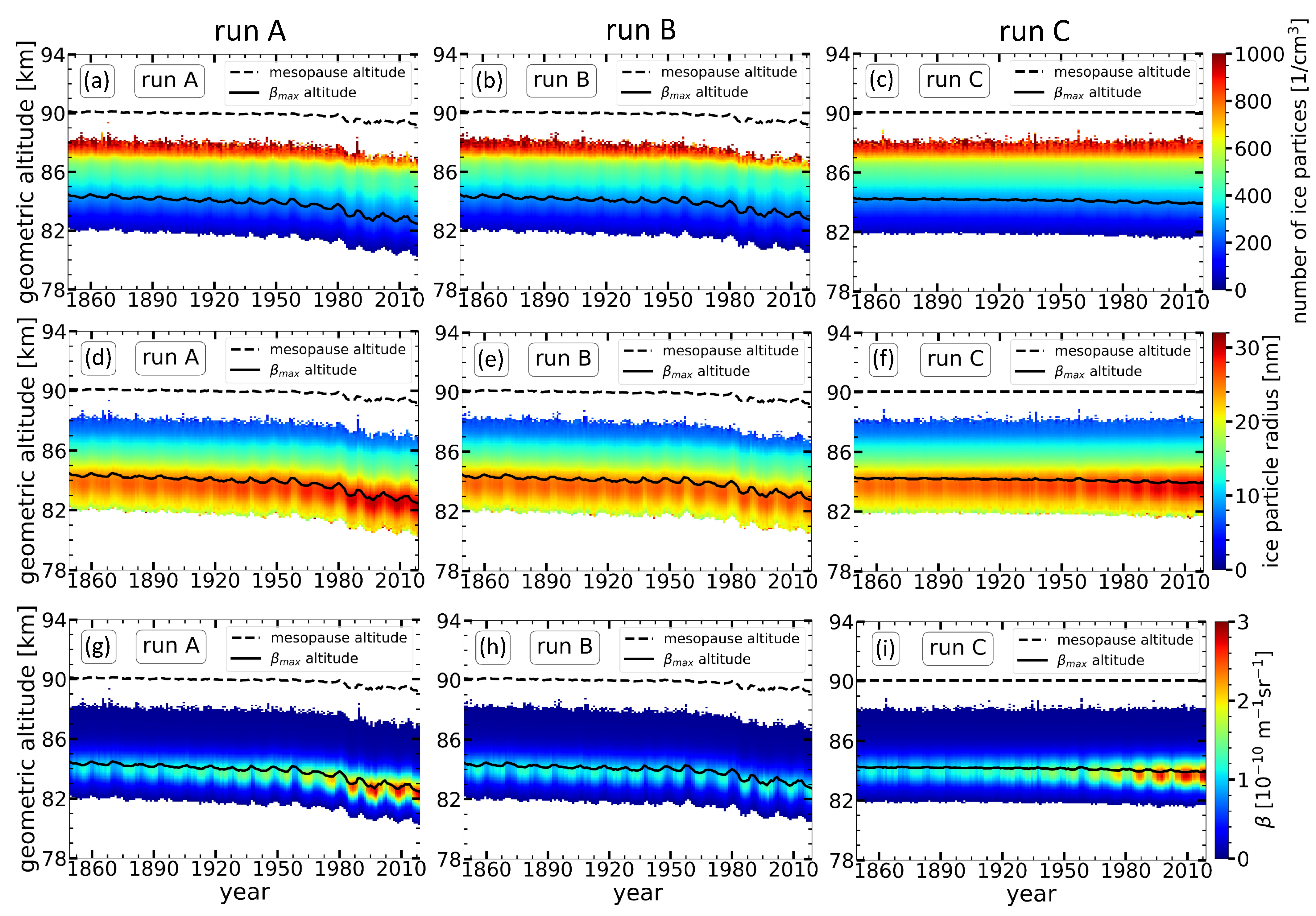
Time series of NLC properties (number of ice particles, ice particle radius and brightness) as a function of geometric altitude, averaged monthly (July) and zonally at 69° N. The results are shown for three runs (see insert). (a–c) Number of ice particles, (d–f) ice particle radius and (g–i) NLC brightness. Only NLC above a brightness threshold (βlim = 0.05) is considered while averaging.
The number of ice particles or the density of ice particles represents the total number of ice particles in a cubic centimetre (cm−3). The trends in the vertical profiles of the number of ice particles show that a significant proportion of the ice particles is located approximately from ~86 km to ~89 km, and this number density decreases with decreasing altitude. The temperature is lowest at higher altitudes around the mesopause height. Regarding water vapour, its concentration decreases with height and is notably low around mesopause altitudes (see Figure 4). The extremely cold temperature at these altitudes causes these regions to become supersaturated, even though the water vapour concentration is very low. Consequently, the ice particles formed at higher altitudes are smaller in size. These ice particles grow by absorbing more H2O from the background during sedimentation and reach their maximum size before their sublimation, which occurs between 82 and 85 km altitude. Regardless of the altitude where the maximum number of ice particles is found, the maximum NLC brightness (βmax) (Figure 5d–f) occurs at the altitude corresponding to the maximum particle radius (Figure 5g–i). This is because the increase in the backscatter cross-section is roughly proportional to the radius raised to the power of six (r6). As a result, higher brightness is linked to larger particle radii, resulting in enhanced light scattering at the altitude where the ice particles reach their maximum radius.
The radius of the NLC ice particles shows an increasing trend in runs A (Figure 5d) and C (Figure 5f), while it does not increase significantly in run B (Figure 5e). This is attributed to the increase in H2O concentration in runs A and C due to the increase in CH4. The increasing availability of water vapour in the background promotes the growth of ice particles and leads to larger ice particle sizes. The ice particle size in run B does not increase significantly because the H2O concentration does not increase due to the constant CH4 concentration. The temporal evolution of the NLC brightness also shows an apparent increase with time for runs A (Figure 5g) and C (Figure 5i). In contrast, it does not increase in run B (Figure 5h). This indicates that the brightness of NLC also increases due to an increase in H2O concentration. It is also noted that the long-term changes in NLC properties are more pronounced at the altitude of the maximum particle radius, especially around the maximum brightness altitude (βmax altitude) indicated by the solid black line.
In Figure 5, we can see the impact of the 11-year solar cycle on the vertical distribution of the NLC properties. During solar minimum, the NLC radius and brightness are larger, while during solar maximum, they are smaller. Less water vapour is available during solar maximum due to increased photolysis and less ice formation growth due to higher temperatures. As a result, smaller ice particles are formed, resulting in less brightness during solar maximum compared to solar minimum years. This effect is visible at all altitudes, with the most significant impact being at the maximum βmax altitude. In runs A and B, the solar cycle influences the lower and upper altitude limits of the NLC layers and the βmax altitude. These parameters respond to the solar cycle by shifting up during the maximum and down during the minimum. In run C, conversely, where there is no temperature change and constant CO2, the lower and upper altitude limits of the NLC layers and the βmax altitude show no significant response to the solar cycle. The mechanism behind this is discussed in more detail in the next section.
3.4. Greenhouse Gas Effects on NLC Solar Cycle Response
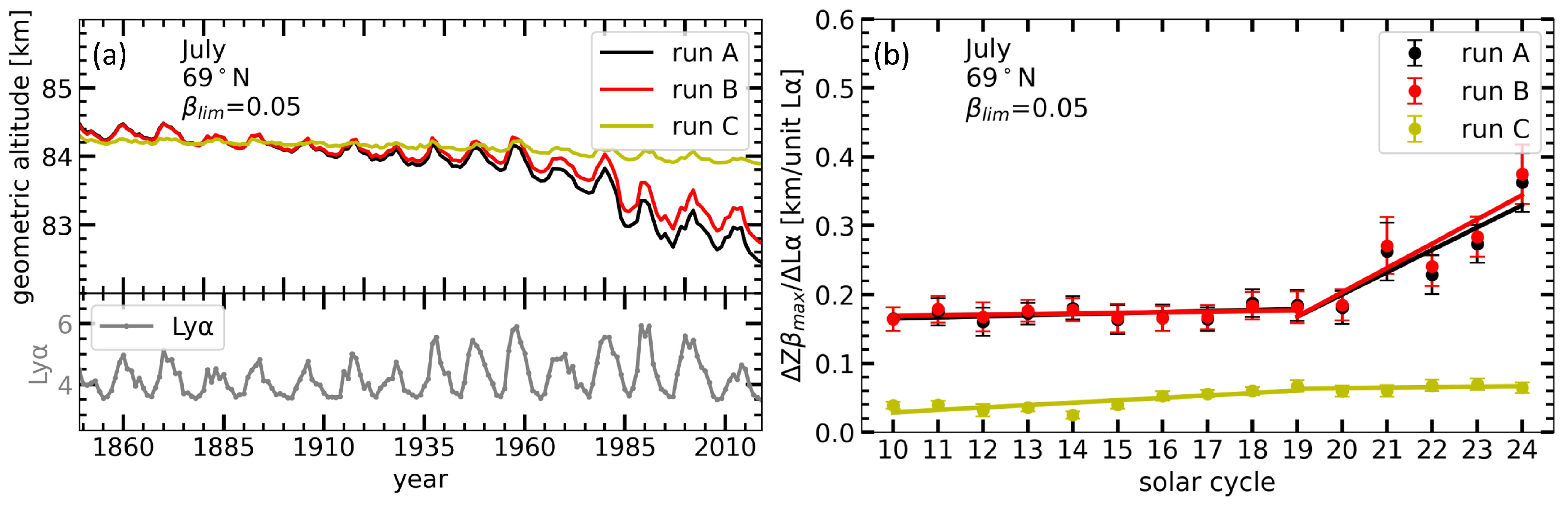
This section analyses the trends in the response of different NLC properties to the 11-year solar cycle. We used MIMAS runs A, B and C to see how the increase in CO2 and CH4 affects the solar cycle response of various NLC properties. We only considered the middle of the summer season, i.e., July. We also applied a threshold in NLC brightness (βlim = 0.05) to exclude non-NLC events while considering even small NLC events [26]. Figure 6a shows the time series of NLC altitude, herein defined as the βmax altitude. The lower panel of Figure 6a shows the time series of Lyα. The NLC altitude decreases in runs A and B due to CO2-induced atmospheric shrinking. In run C, where only H2O increases, the NLC altitude remains nearly constant [9,20]. The decrease in NLC altitudes in MIMAS is consistent with long-term radio wave reflectivity altitude observations dating back to 1959 (see Figure 2a in [23]). Figure 6a shows that run A and B show a significant modulation in NLC altitude according to the solar cycle, while run C shows very small modulation. In particular, the NLC altitude positively responds to the solar cycle by an upward shift during solar maximum and a downward shift during solar minimum. This is because the Earth’s upper atmosphere heats up during solar maximum due to the Sun’s higher energy flux, which causes the background temperature to rise and the mesosphere to expand. The rise in temperature shifts the lower altitude limit of the supersaturated region (where S = 1) upwards, which in turn causes an upward shift of the NLC layers. The slight positive response of the NLC altitude in run C is primarily due to the solar cycle-induced photolysis effect on water vapour. The increase in H2O photolysis during solar maximum reduces the background H2O. As the H2O concentration decreases, the saturation ratio (S) decreases, which causes a slight upward shift of the lower altitude limit of the supersaturated region (where S = 1). Compared to the photolysis effect on H2O, the temperature changes have a larger impact on the saturation ratio ([21]) and, thus, on the altitude range of the supersaturated region. For this reason, the NLC altitude response in run C (constant temperature) is very small compared to runs A and B.
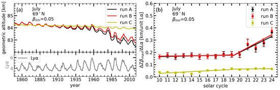
Figure 6.
(a) Time series of NLC altitudes (averaged for July and zonally at 69° N) from 1849 to 2019. The results from three runs (A, B and C) are shown in the figure (see insert). The lower panel shows the time series of the solar Lyα flux (unit: 1011 γcm−2s−2) averaged for July. (b) Response of NLC altitude to the unit change in solar Lyα during solar cycles between 1855 and 2019 (for example, solar cycle 10 corresponds to 1855–1867, while solar cycle 24 represents 2008–2019). The three runs, A, B and C, are shown (see insert) along with linear regression fits. The error bars represent the standard error of the mean for the respective solar cycle years.
To investigate trends in the variation of NLC altitude to the solar cycle, we calculated the response of the NLC altitude to a unit change in Lyα for each solar cycle. To do this, we calculated the absolute difference in NLC altitude between the solar maximum and minimum and divided it by the absolute Lyα difference between the corresponding solar maximum and minimum. Figure 6b presents the time series of the response of NLC altitude for 15 solar cycles from 1855 to 2019. Before the 19th solar cycle (1954–1964), the response of NLC altitude showed a relatively slow and gradual increase. However, after the 19th solar cycle, there is an acceleration in the response of NLC altitude. After 1960, several properties of NLC, including brightness, radius and IWC, experienced an amplification due to the accelerated increase in greenhouse gas concentrations [9,20]. Therefore, we show linear fit lines for the responses before and after the 19th solar cycle.
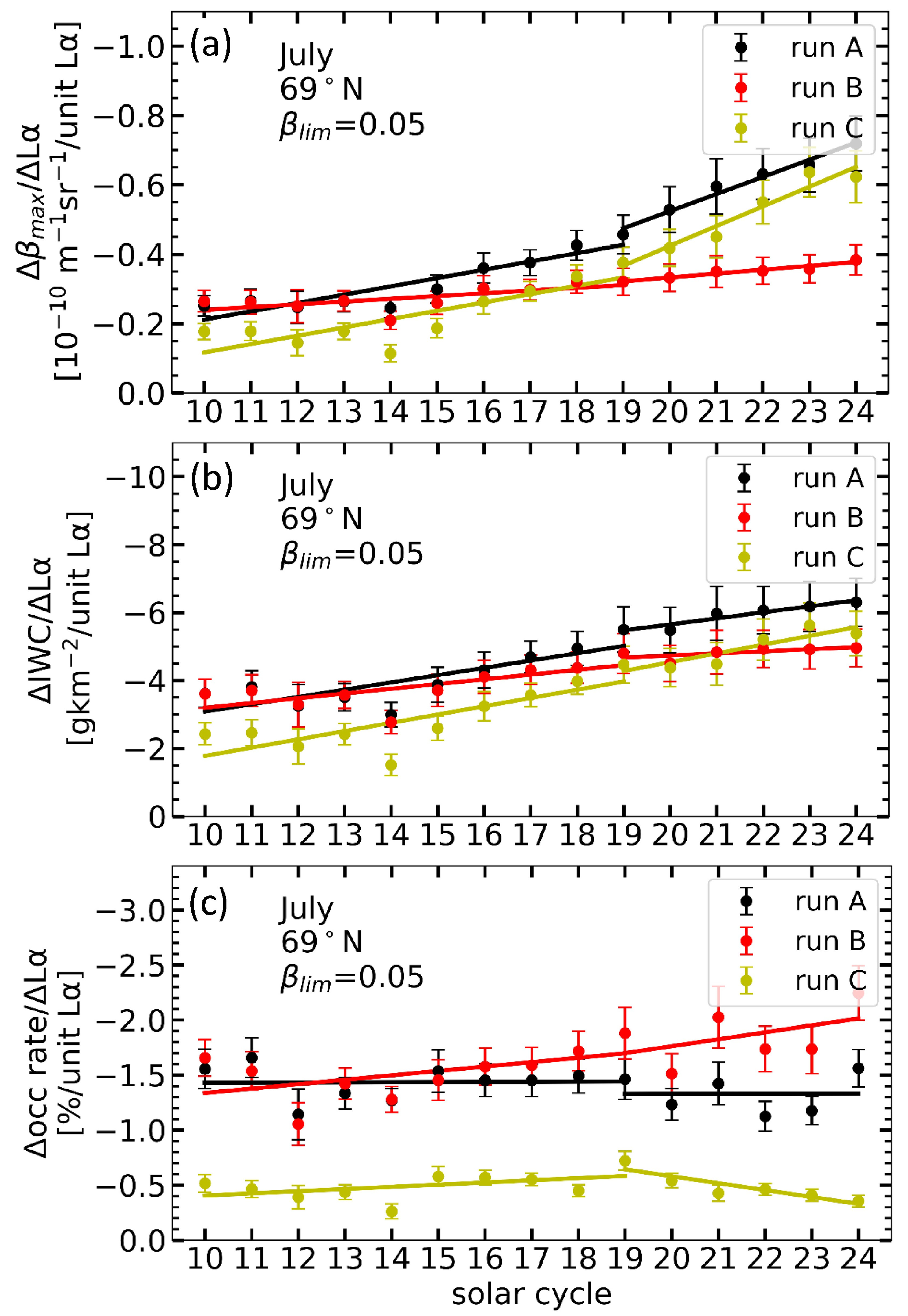
We also calculated the solar cycle response of maximum NLC brightness, IWC and NLC occurrence (Figure 7). Figure 7a shows the time series of the solar cycle response of maximum brightness for runs A, B and C. The maximum brightness shows a negative response to the solar cycle variations, and its magnitude increases with time in all runs. However, the magnitude of this increase is more pronounced in runs A and C than in run B. This indicates that an increase in H2O content is the main factor for the increase in the solar cycle response of NLC brightness. Compared to run C, the higher response in run A can be attributed to the combined effects of CO2 increase, temperature changes and H2O increase. In contrast, run C uses constant temperature and CO2 conditions for all years. In run A, the negative response of maximum brightness increases from about −0.25 (10−10 m−1sr−1/unit Lyα) in the 10th solar cycle to −0.75 (10−10 m−1sr−1/unit Lyα) in the 24th solar cycle.
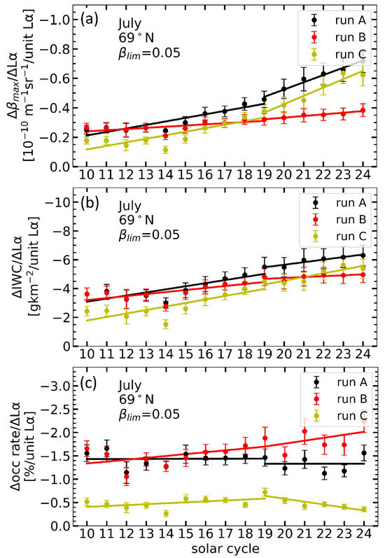
Figure 7.
NLC properties response to a unit change in solar Lyα at 69° N during solar cycles between 1855 and 2019. Results are shown for three runs, A, B and C (see insert). Error bars indicate the standard error of the mean during respective solar cycle years. The figures are shown for (a) maximum brightness, (b) IWC and (c) NLC occurrence rate, with a threshold value of βlim = 0.05 applied.
Figure 7b shows an increasing trend in the magnitude of the response of IWC to the solar cycle in all runs. During the 10th solar cycle, runs A and B have almost identical magnitude of responses to the solar cycle, which are higher than those of run C. In the 22nd solar cycle, the response of IWC to the solar cycle in run C exceeds that of run B. The results suggest that both temperature variations and increasing H2O contribute to the increase in the response of IWC to the solar cycle. However, the influence of H2O has a more significant impact on the increased response of IWC than the effects of CO2 and temperature. The SBUV satellite has provided the longest dataset of satellite observations for NLC from 1979 to the present, covering latitudes from about 55° N to 82° N in both the Northern and Southern Hemispheres [13]. Our recent study [17] compared the IWC response of MIMAS and SBUV. We found a good agreement in both the anti-correlation pattern and the magnitude of the solar cycle-induced modulation. Moreover, the SOFIE/AIM instrument measured a mean value of IWC ~ 59 g/km2 at mid-latitudes in July 2015, using a threshold value of IWC > 40 g/km2 (see Figure 3 in [35]). This perfectly agrees with the IWC values from MIMAS, namely IWC ~ 58–59 g/km2 (Figure 3c in [9]), using the same threshold value. This agreement shows the potential of our model to study the response of IWC to the solar cycle [17].
Figure 7c presents the trends in the solar cycle response of the NLC occurrence rate. The occurrence rate of NLC is calculated as follows: For July in each year, the total number of latitude/longitude fields (referred to as “events”, Nmax) is determined by latitude fields (6), longitude fields (120) and time windows of 6 h each (31 days × 4 per day = 124-time steps), resulting in a total number of 89,280 events (Nmax). Whenever an ice layer occurs (applying a given threshold in NLC brightness (βlim = 0.05)) in a given latitude/longitude bin and time segment in MIMAS, we call this an “NLC event”. The NLC occurrence rate is calculated by dividing the number of NLC events by the total number of events (Nmax). The occurrence rate of NLC shows a negative response to the solar cycle. Figure 7c shows that the response of NLC occurrence to the solar cycle is more significant when temperature changes (runs A and B) compared to constant temperature (run C). This suggests that solar cycle temperature variations significantly influence the NLC occurrence rate. This is a consequence of the transition of NLC events to non-NLC events (from super- to sub-saturation), which primarily depends on temperature variation, whereas water vapour is of secondary importance [21]. The response is higher in run B than in run A. In run A, the increase in water vapour leads to an increase in the saturation ratio of events. In run B, where the background H2O remains constant, a considerable fraction of events have a low saturation ratio close to one. Therefore, in run B, even a small increase or decrease in temperature during solar maximum or minimum significantly impacts the saturation ratio (S), affecting the transition of many NLC events from super- to sub-saturation and, consequently, NLC occurrence.
We find that the response of the NLC occurrence rate after the 19th solar cycle in runs A and C remains roughly constant or decreases slightly. This is because, after the 19th solar cycle, the accelerated increase in carbon dioxide (CO2) contributes to the cooling of the upper mesosphere, and the increase in methane (CH4) leads to higher concentrations of water vapour. Consequently, more “events” become “NLC events”, and the saturation ratio (S) of these NLC events becomes large. In such cases, the variations in background H2O and temperature caused by the solar cycle have little effect on the transition of NLC events from super- to sub-saturation, as the saturation ratio is already very large (S >> 1). For this reason, the response of the occurrence rate of NLC decreases slightly from the 19th solar cycle onwards. It is important to note that the results may vary with a different βlim. For example, the IWC and NLC occurrence rate trends can differ significantly depending on the βlim applied (see Figures 9 and 10 of [20]).
3.5. Solar Cycle Response of NLC at Different Latitudes
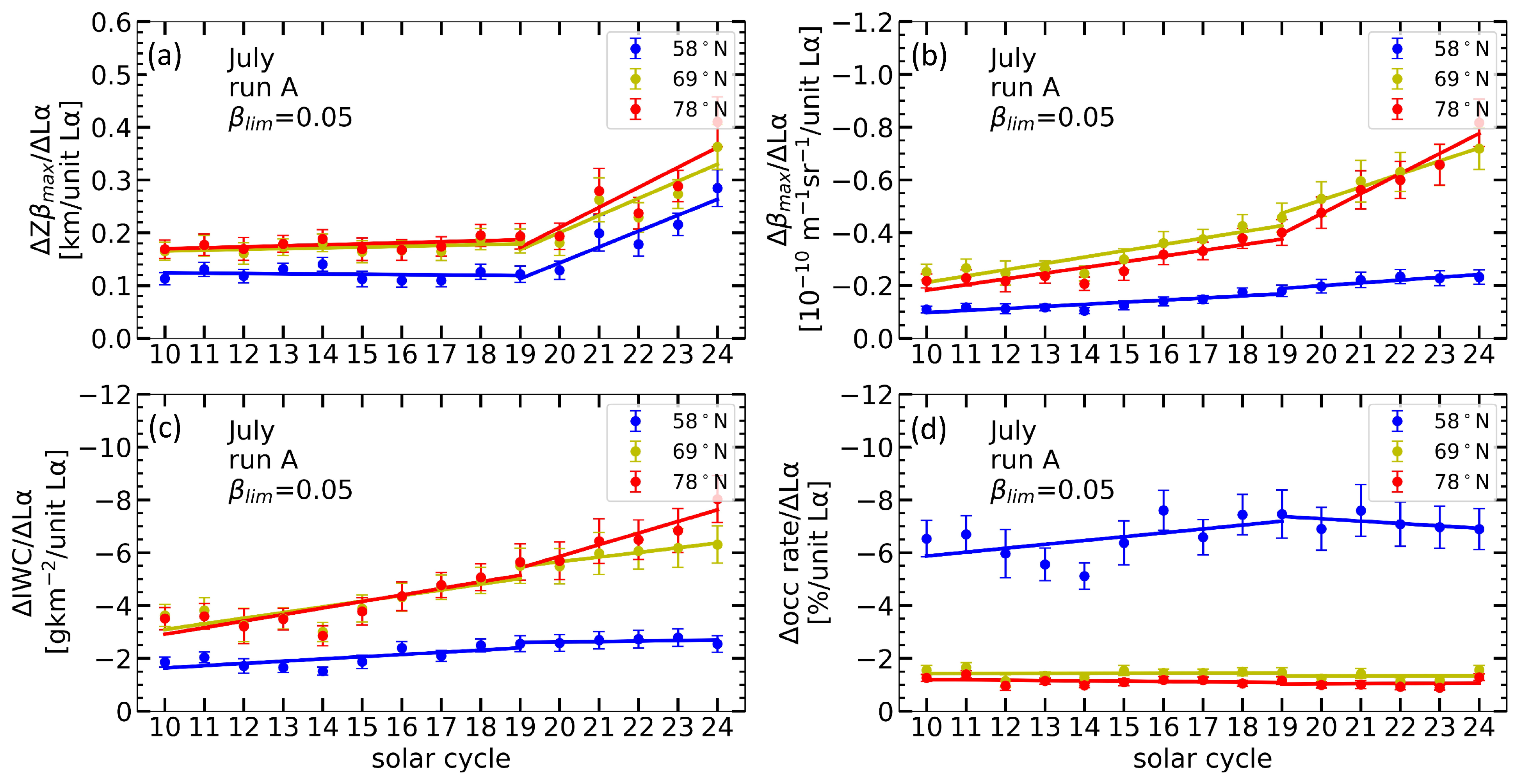
In this section, we investigate how the response of NLC to the solar cycle varies with latitude. For this study, we used MIMAS run A only and calculated the response of NLC properties at latitudes 58 ± 3° N (middle), 69 ± 3° N (high) and 78 ± 3° N (arctic). Figure 8 shows the time series of the solar cycle response of different NLC properties at middle, high and arctic latitudes. The trends in solar cycle response of NLC altitude, maximum brightness and IWC are larger and similar at high and arctic latitudes compared to those at mid-latitudes. The study on NLC trends by [20] also shows that most NLC parameters behave similarly at high and arctic latitudes.
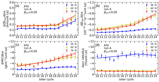
Figure 8.
NLC properties response to a unit change in solar Lyα during solar cycles between 1855 and 2019. Results are shown for three latitudes (see insert). Error bars indicate the standard error of the mean during respective solar cycle years. The figures are shown for (a) NLC altitude, (b) maximum brightness, (c) IWC and (d) NLC occurrence rate, with a threshold value of βlim = 0.05 applied.
In Figure 8a, the NLC altitude positively responds to the solar cycle. As already explained, the primary factor influencing the response of NLC altitude is the temperature change caused by the solar cycle. The temperature response to the solar cycle varies with latitude. During periods of high solar activity, the mesospheric temperature generally increases. This response is usually weaker at mid-latitudes than at higher latitudes, as solar radiation penetrates the mesosphere more directly at higher latitudes, leading to greater warming. In contrast, solar radiation at mid-latitudes has a relatively weaker influence on the mesosphere temperature. The lower response of NLC altitudes to the solar cycle at mid-latitudes can be attributed to the lower temperature response at mid-latitudes compared to high and arctic latitudes. In Figure 8a, the increase in response (the slope of the regression lines) at mid-latitudes is almost similar to that at high and arctic latitudes. The similarity of the trends in NLC altitude response at all latitudes results from the fact that the temperature trends at NLC altitudes are almost independent of latitude (see Figure 2 in [12] and Figure 7a in [20]).
For maximum brightness and IWC (Figure 8b,c), the response is significantly higher at high and arctic latitudes than at mid-latitudes. As we have already discussed, H2O is the main factor influencing the changes in NLC brightness and IWC. At high and arctic latitudes, the extremely low temperatures in the mesopause region in summer and the relatively high water vapour concentrations lead to a larger saturation ratio [37]. Due to these favourable background conditions, more NLC are formed, and NLC brightness and IWC show a significant response to the solar cycle at high and arctic latitudes.
The response of NLC occurrence to the solar cycle is very large at mid-latitudes compared to high and arctic latitudes (Figure 8d). Due to the lower temperatures and relatively high water vapour concentration, the saturation ratio and occurrence rate of NLC are greater at high and arctic latitudes (>80%) than at mid-latitudes (30–60%) (see Figure 10a in [20]). Due to this high saturation ratio of NLC events, the temperature and water vapour changes during the solar cycle need to be more significant to transition from super- to sub-saturation of many NLC events. In mid-latitudes, on the other hand, where NLC occur less frequently due to warmer temperatures (close to frost point temperature) and less water vapour, temperature changes play a critical role in the degree of water vapour saturation. Thus, even slight variations in temperature and water vapour caused by the solar cycle can significantly impact the occurrence of NLC in mid-latitudes. This is why the response of NLC occurrence to the solar cycle is more significant at the mid-latitudes. However, after 1960, this response of occurrence rate at mid-latitudes started to decrease due to accelerated cooling by CO2 and increasing H2O, which increases the saturation ratio of events. Therefore, the effect of the solar cycle started to decrease in the NLC occurrence rate at mid-latitudes after the year 1960. In the future, due to further increases in greenhouse gases, NLC occurrence will increase further, and we expect to see a diminishing solar cycle response of NLC occurrence at all latitudes.
4. Conclusions
Anthropogenic emissions of CO2 and CH4 have been increasing over time, with the rate of increase accelerating since 1960. These effects are largely associated with climate change due to their global warming potential. However, in the upper atmosphere, the effects are different. An increase in greenhouse gases leads to a cooling of the upper mesosphere because of an increased escape of infrared photons into space (Luebken et al., 2018). Nevertheless, the implications of this for the upper mesosphere are poorly understood due to difficulties and limitations in measuring atmospheric properties. NLC have been proposed as a key tracer in the summer mesopause region due to their high sensitivity to background atmospheric conditions, including temperature, water vapour concentration and dynamics. Therefore, NLC have been used as the primary indicator of changes in the upper mesosphere and have been the subject of several studies [9,20,38,39,40,41,42,43,44]. In this study, the long-term trends in the response of NLC properties and the background atmosphere to the solar cycle are investigated during the period 1849–2019 (see also Supplementary Materials), which covers 15 complete solar cycles (solar cycle 10 to solar cycle 24). We summarise our results by answering the questions raised in the introduction as follows:
- (1)
- Background temperature and H2O show an apparent response to the solar cycle throughout the study period, which intensified after 1960 due to increased greenhouse gas emissions. The temperature response at a given geometric altitude increases due to atmospheric shrinking caused by increased CO2. The increase in the response of water vapour to the solar cycle is mainly due to the increase in CH4, which leads to the production of more H2O through oxidation.
- (2)
- We found solar cycle responses in the vertical distribution profiles of ice particle number, mean radius and NLC brightness. The solar cycle influence is present at all altitudes and peaks at the altitude of maximum NLC brightness. The magnitude of the ice particle radius and brightness response increases with time, mainly due to the increase of H2O, while the downward shift of the profiles is due to atmospheric shrinking.
- (3)
- The properties of NLC, such as maximum brightness, mean radius of ice particles, IWC and occurrence rate, respond to the solar cycle, and these responses increase with time mainly due to an increase in water vapour. The response in NLC altitudes occurs mainly due to solar cycle-induced temperature variation. The upward shift in NLC altitudes is due to the expansion of the atmosphere due to increased heating during solar maximum.
- (4)
- The enhancement in response of NLC brightness and ice water content (IWC) to the solar cycle is primarily due to an increase in CH4, which leads to an increase in H2O. On the other hand, the increase in response of NLC altitude is due to an increase in CO2, which leads to a larger response of the background temperature to the solar cycle.
- (5)
- The solar cycle response of NLC properties differs at different latitudes. NLC height, maximum brightness and ice water content are more responsive at high and arctic latitudes and show a similar trend. However, NLC occurrence is less responsive at high and arctic latitudes but much more responsive at mid-latitudes. The saturation ratio of NLC events is higher at high and arctic latitudes, while they are relatively low at mid-latitudes due to higher temperatures and lower water vapour concentrations. Consequently, temperature and water vapour variations during the solar cycle have a greater influence on the occurrence of NLC at mid-latitudes than at high and arctic latitudes.
We found that the increase in greenhouse gas concentrations is primarily responsible for the enhanced response of noctilucent clouds to the solar cycle, illustrating the impact of increasing anthropogenic emissions on temperature and water vapour concentration in the upper atmosphere. Given the important role that the solar cycle plays in the Earth’s atmosphere, a detailed understanding of its impact on the upper mesosphere is crucial for improving climate modelling. For example, the response of H2O to the solar cycle under NLC conditions shows a positive value at NLC-forming altitudes and a negative value at NLC-sublimating altitudes. This information could be taken into account in future developments of atmospheric models, especially for the chemical component, as water vapour plays an important role in the chemistry of the upper mesosphere. In addition, NLC are located at transition altitudes from the atmosphere to space, which are critical for satellites. The changes and enhancements in NLC properties could provide observational evidence of changes in the atmosphere at hard-to-measure altitudes. All these results show that climate change is more pronounced in the upper mesosphere, which can be directly observed from Earth through NLC. Consequently, these results point to the need to reduce greenhouse gas emissions by taking action and implementing appropriate strategies.
Supplementary Materials
The following supporting information can be downloaded at: https://www.mdpi.com/article/10.3390/atmos15010088/s1, Table S1. A table presenting the definitions of technical terms used in the article; Figure S1. Time series of background temperature and H2O at the maximum brightness altitude for three different latitudes (58° N, 69° N, and 78° N) spanning the years 1849 to 2010; Figure S2. Time series of NLC properties (see y-axis label) for three different latitudes (58° N, 69° N, and 78° N) spanning the years 1849 to 2010.
Author Contributions
M.G. conducted LIMA model simulations; A.V. conducted MIMAS model simulations and wrote the first draft of the paper; A.V., G.B., M.G. and F.-J.L. interpreted the results and contributed significantly to the interpretation and improvement of the paper. All authors have read and agreed to the published version of the manuscript.
Funding
This research was funded by the TIMA project of the BMBF (Bundesministerium für Bildung und Forschung) research initiative ROMIC (grant no. 01LG1902A).
Institutional Review Board Statement
Not applicable.
Informed Consent Statement
Not applicable.
Data Availability Statement
Lyman-α data are available at http://lasp.colorado.edu/lisird/lya/ (accessed on 10 November 2023) from LASP. The data utilised in this manuscript can be downloaded from https://www.radar-service.eu/radar/en/dataset/xqHORiMNGebILWkX?token=WOVCiyZPRkGXlBdpgcnU (accessed on 10 November 2023).
Acknowledgments
We would like to thank Corinna Schütt for her support in working with the LIMA model script. We acknowledge the Mauna Loa records for CO2 and CH4 from http://www.esrl.noaa.gov/gmd/ccgg/, last access: 16 November 2023.
Conflicts of Interest
The contact author has declared that none of the authors have any competing interests.
References
- Garcia, R.R. Dynamics, Radiation, and Photochemistry in the Mesosphere: Implications for the Formation of Noctilucent Clouds. J. Geophys. Res. Atmos. 1989, 94, 14605–14615. [Google Scholar] [CrossRef]
- Berger, U.; von Zahn, U. Three-Dimensional Modeling of the Trajectories of Visible Noctilucent Cloud Particles: An Indication of Particle Nucleation Well below the Mesopause. J. Geophys. Res. Atmospheres 2007, 112, D16204. [Google Scholar] [CrossRef]
- Gadsden, M.; Schröder, W. Noctilucent Clouds; Physics and Chemistry in Space Planetology; Springer: Berlin/Heidelberg, Germany, 1989; ISBN 978-3-540-50685-0. [Google Scholar]
- Gadsden, M. A Secular Change in Noctilucent Cloud Occurrence. J. Atmos. Terr. Phys. 1990, 52, 247–251. [Google Scholar] [CrossRef]
- Thomas, G.E.; Olivero, J. Noctilucent Clouds as Possible Indicators of Global Change in the Mesosphere. Adv. Space Res. 2001, 28, 937–946. [Google Scholar] [CrossRef]
- Thomas, G.E. Is the polar mesosphere the miner’s canary of global change? Adv. Space Res. 1996, 18, 149–158. [Google Scholar] [CrossRef]
- Thomas, G.E. Are Noctilucent Clouds Harbingers of Global Change in the Middle Atmosphere? Adv. Space Res. 2003, 32, 1737–1746. [Google Scholar] [CrossRef]
- Hervig, M.E.; Berger, U.; Siskind, D.E. Decadal Variability in PMCs and Implications for Changing Temperature and Water Vapor in the Upper Mesosphere. J. Geophys. Res. 2016, 121, 2383–2392. [Google Scholar] [CrossRef]
- Lübken, F.J.; Berger, U.; Baumgarten, G. On the Anthropogenic Impact on Long-Term Evolution of Noctilucent Clouds. Geophys. Res. Lett. 2018, 45, 6681–6689. [Google Scholar] [CrossRef]
- DeLand, M.T.; Shettle, E.P.; Thomas, G.E.; Olivero, J.J. A Quarter-Century of Satellite Polar Mesospheric Cloud Observations. J. Atmos. Sol.-Terr. Phys. 2006, 68, 9–29. [Google Scholar] [CrossRef]
- Von Zahn, U.; Berger, U. Persistent Ice Cloud in the Midsummer Upper Mesosphere at High Latitudes: Three-Dimensional Modeling and Cloud Interactions with Ambient Water Vapor. J. Geophys. Res. Atmos. 2003, 108. [Google Scholar] [CrossRef]
- Lübken, F.J.; Berger, U.; Baumgarten, G. Temperature Trends in the Midlatitude Summer Mesosphere. J. Geophys. Res. Atmos. 2013, 118, 13347–13360. [Google Scholar] [CrossRef]
- Hervig, M.E.; Siskind, D.E.; Bailey, S.M.; Merkel, A.W.; DeLand, M.T.; Russell, J.M. The Missing Solar Cycle Response of the Polar Summer Mesosphere. Geophys. Res. Lett. 2019, 46, 10132–10139. [Google Scholar] [CrossRef]
- DeLand, M.T.; Shettle, E.P.; Thomas, G.E.; Olivero, J.J. Solar Backscattered Ultraviolet (SBUV) Observations of Polar Mesospheric Clouds (PMCs) over Two Solar Cycles. J. Geophys. Res. Atmos. 2003, 108, 8445. [Google Scholar] [CrossRef]
- Hervig, M.; Siskind, D. Decadal and Inter-Hemispheric Variability in Polar Mesospheric Clouds, Water Vapor, and Temperature. J. Atmos. Sol.-Terr. Phys. 2006, 68, 30–41. [Google Scholar] [CrossRef]
- Siskind, D.E.; Stevens, M.H.; Hervig, M.E.; Randall, C.E. Recent Observations of High Mass Density Polar Mesospheric Clouds: A Link to Space Traffic? Geophys. Res. Lett. 2013, 40, 2813–2817. [Google Scholar] [CrossRef]
- Vellalassery, A.; Baumgarten, G.; Grygalashvyly, M.; Lübken, F.-J. Greenhouse Gas Effects on the Solar Cycle Response of Water Vapour and Noctilucent Clouds. Ann. Geophys. 2023, 41, 289–300. [Google Scholar] [CrossRef]
- Nedoluha, G.E.; Kiefer, M.; Lossow, S.; Michael Gomez, R.; Kämpfer, N.; Lainer, M.; Forkman, P.; Martin Christensen, O.; Jin Oh, J.; Hartogh, P.; et al. The SPARC Water Vapor Assessment II: Intercomparison of Satellite and Ground-Based Microwave Measurements. Atmos. Chem. Phys. 2017, 17, 14543–14558. [Google Scholar] [CrossRef]
- Hervig, M.E.; Siskind, D.E.; Bailey, S.M.; Russell, J.M. The Influence of PMCs on Water Vapor and Drivers behind PMC Variability from SOFIE Observations. J. Atmos. Sol.-Terr. Phys. 2015, 132, 124–134. [Google Scholar] [CrossRef]
- Lübken, F.J.; Baumgarten, G.; Berger, U. Long Term Trends of Mesopheric Ice Layers: A Model Study. J. Atmos. Sol.-Terr. Phys. 2021, 214, 105378. [Google Scholar] [CrossRef]
- Berger, U.; Von Zahn, U. Icy Particles in the Summer Mesopause Region: Three-Dimensional Modeling of Their Environment and Two-Dimensional Modeling of Their Transport. J. Geophys. Res. Space Phys. 2002, 107, SIA-10. [Google Scholar] [CrossRef]
- Berger, U. Modeling of Middle Atmosphere Dynamics with LIMA. J. Atmos. Sol.-Terr. Phys. 2008, 70, 1170–1200. [Google Scholar] [CrossRef]
- Berger, U.; Lübken, F.J. Mesospheric Temperature Trends at Mid-Latitudes in Summer. Geophys. Res. Lett. 2011, 38, L22804. [Google Scholar] [CrossRef]
- Machol, J.; Snow, M.; Woodraska, D.; Woods, T.; Viereck, R.; Coddington, O. An Improved Lyman-Alpha Composite. Earth Space Sci. 2019, 6, 2263–2272. [Google Scholar] [CrossRef]
- Compo, G.P.; Whitaker, J.S.; Sardeshmukh, P.D.; Matsui, N.; Allan, R.J.; Yin, X.; Gleason, B.E.; Vose, R.S.; Rutledge, G.; Bessemoulin, P.; et al. The Twentieth Century Reanalysis Project. Q. J. R. Meteorol. Soc. 2011, 137, 1–28. [Google Scholar] [CrossRef]
- WMO. Statement on the Status of the Global Climate in 2011; World Meteorological Organization: Geneva, Switzerland, 2012; ISBN 978-92-63-11085-5. [Google Scholar]
- Etheridge, D.; Barnola, J.; Morgan, V.; Steele, L.; Langenfelds, R.; Francey, R. Historical CO2 Records from the Law Dome DE08, DE08-2, and DSS Ice Cores (1006 A.D.-1978 A.D); Oak Ridge National Laboratory, U.S. Department of Energy: Oak Ridge, TN, USA, 1998.
- Yiğit, E.; Medvedev, A.S. Extending the Parameterization of Gravity Waves into the Thermosphere and Modeling Their Effects. In Climate and Weather of the Sun-Earth System (CAWSES) Highlights from a Priority Program; Springer: Dordrecht, The Netherlands, 2013; pp. 467–480. [Google Scholar]
- Butchart, N. The Brewer-Dobson Circulation. Rev. Geophys. 2014, 52, 157–184. [Google Scholar] [CrossRef]
- Kiliani, J. 3-D Modeling of Noctilucent Cloud Evolution and Relationship to the Ambient Atmosphere. Ph.D. Thesis, IAP. University of Rostock, Kühlungsborn, Germany, 2014. [Google Scholar]
- Roble, R.G.; Dickinson, R.E. How will changes in carbon dioxide and methane modify the mean structure of the mesosphere and thermosphere? Geophys. Res. Lett. 1989, 46, 1441–1444. [Google Scholar] [CrossRef]
- Garcia, R.R.; Marsh, D.R.; Kinnison, D.E.; Boville, B.A.; Sassi, F. Simulation of Secular Trends in the Middle Atmosphere, 1950–2003. J. Geophys. Res. Atmos. 2007, 112, D09301. [Google Scholar] [CrossRef]
- Marsh, D.R.; Mills, M.J.; Kinnison, D.E.; Lamarque, J.F.; Calvo, N.; Polvani, L.M. Climate Change from 1850 to 2005 Simulated in CESM1(WACCM). J. Clim. 2013, 26, 7372–7391. [Google Scholar] [CrossRef]
- Keckhut, P.; Wild, J.D.; Gelman, M.; Miller, A.J.; Hauchecorne, A. Investigations on Long-term Temperature Changes in the Upper Stratosphere Using Lidar Data and NCEP Analyses. J. Geophys. Res. Atmos. 2001, 106, 7937–7944. [Google Scholar] [CrossRef]
- Hervig, M.E.; Gerding, M.; Stevens, M.H.; Stockwell, R.; Bailey, S.M.; Russell, J.M.; Stober, G. Mid-Latitude Mesospheric Clouds and Their Environment from SOFIE Observations. J. Atmos. Sol.-Terr. Phys. 2016, 149, 1–14. [Google Scholar] [CrossRef]
- Remsberg, E. Observation and Attribution of Temperature Trends Near the Stratopause From HALOE. J. Geophys. Res. Atmos. 2019, 124, 6600–6611. [Google Scholar] [CrossRef] [PubMed]
- Körner, U.; Sonnemann, G.R. Global Three-dimensional Modeling of the Water Vapor Concentration of the Mesosphere-mesopause Region and Implications with Respect to the Noctilucent Cloud Region. J. Geophys. Res. Atmos. 2001, 106, 9639–9651. [Google Scholar] [CrossRef]
- Hansen, G.; Von Zahn, U. Simultaneous Observations of Noctilucent Clouds and Mesopause Temperatures by Lidar. J. Geophys. Res. Atmos. 1994, 99, 18989–18999. [Google Scholar] [CrossRef]
- Nussbaumer, V.; Fricke, K.H.; Langer, M.; Singer, W.; Von Zahn, U. First Simultaneous and Common Volume Observations of Noctilucent Clouds and Polar Mesosphere Summer Echoes by Lidar and Radar. J. Geophys. Res. Atmos. 1996, 101, 19161–19167. [Google Scholar] [CrossRef]
- Von Cossart, G.; Hoffmann, P.; Von Zahn, U.; Keckhut, P.; Hauchecorne, A. Mid-latitude Noctilucent Cloud Observations by Lidar. Geophys. Res. Lett. 1996, 23, 2919–2922. [Google Scholar] [CrossRef]
- Von Zahn, U.; Von Cossart, G.; Fiedler, J.; Rees, D. Tidal Variations of Noctilucent Clouds Measured at 69° N Latitude by Groundbased Lidar. Geophys. Res. Lett. 1998, 25, 1289–1292. [Google Scholar] [CrossRef]
- Karlsson, B.; Rapp, M. Latitudinal Dependence of Noctilucent Cloud Growth. Geophys. Res. Lett. 2006, 33, 2006GL025805. [Google Scholar] [CrossRef]
- Hultgren, K.; Körnich, H.; Gumbel, J.; Gerding, M.; Hoffmann, P.; Lossow, S.; Megner, L. What Caused the Exceptional Mid-Latitudinal Noctilucent Cloud Event in July 2009? J. Atmos. Sol.-Terr. Phys. 2011, 73, 2125–2131. [Google Scholar] [CrossRef]
- Kaifler, N.; Kaifler, B.; Wilms, H.; Rapp, M.; Stober, G.; Jacobi, C. Mesospheric Temperature during the Extreme Midlatitude Noctilucent Cloud Event on 18/19 July 2016. J. Geophys. Res. Atmos. 2018, 123, 13775–13789. [Google Scholar] [CrossRef]

Disclaimer/Publisher’s Note: The statements, opinions and data contained in all publications are solely those of the individual author(s) and contributor(s) and not of MDPI and/or the editor(s). MDPI and/or the editor(s) disclaim responsibility for any injury to people or property resulting from any ideas, methods, instructions or products referred to in the content. |
© 2024 by the authors. Licensee MDPI, Basel, Switzerland. This article is an open access article distributed under the terms and conditions of the Creative Commons Attribution (CC BY) license (https://creativecommons.org/licenses/by/4.0/).