Enhanced Wind-Field Detection Using an Adaptive Noise-Reduction Peak-Retrieval (ANRPR) Algorithm for Coherent Doppler Lidar

Abstract

Wind fields provide direct power for exchanging energy and matter in the atmosphere. All-fiber coherent Doppler lidar is a powerful tool for detecting boundary-layer wind fields. According to the characteristics of the lidar echo signal, an adaptive noise-reduction peak retrieval (ANRPR) algorithm is proposed in this study. Firstly, the power spectrum data are divided into several continuous range gates according to the time series. Then, the adaptive iterative reweighted penalized least-squares (airPLS) method is used to reduce the background noise. Secondly, the continuity between spectra is enhanced by 2D Gaussian low-pass filtering. Finally, an adaptive peak-retrieval algorithm is employed to extract the Doppler shift, facilitating the synthesis of a spatial atmospheric 3D wind field through the vector synthesis method. When comparing data from different heights of the meteorological gradient tower, both the horizontal wind-speed correlation and the horizontal wind-direction correlation exceed 0.90. Experimental results show that the proposed algorithm has better robustness and a longer detection distance than the traditional algorithm.

1. Introduction

Wind-field detection plays a crucial role in atmospheric research by providing essential parameters for meteorology [1]. It not only supports the development of weather forecasting [2] and climate modeling but also plays a significant role in monitoring air pollution [3], preventing weather disasters [4], and facilitating the development of renewable energy [5]. Coherent Doppler lidar (CDL), due to its advantages of high precision, large spatial coverage, and long detection range, is widely employed in atmospheric wind-field detection [4,6].

The CDL receives the echo signal, which is Doppler-shifted due to the Doppler effect of the atmosphere [7]. Doppler shift estimation is conducted by fast Fourier transforming (FFT) the lidar echo signal to obtain the spectrogram, and then the peak detection of the spectrogram is undertaken to obtain the Doppler shift [8]. Given that lidar echo spectra frequently encounter interference from diverse noise sources, with instrumental noise being particularly prominent, the imperative lies in the eradication of this noise and the subsequent extraction of spectral peaks [9]. Therefore, how to estimate the Doppler shift efficiently and accurately becomes the primary task of CDL signal processing.

In previous studies, since the signal becomes increasingly weaker as the range gates increase, it was assumed that the last range gate did not contain a signal component [10,11]. Therefore, the power spectrum of the range gate in the tail sample of the lidar is considered to be a noise background. The effect of removing the background noise is often achieved by subtracting the spectrum of the last range gate from the preceding range gates, i.e., the periodogram method (PM) [12], but, due to the unbalanced nature of the noise and the volatility and randomness of the data, it is bound to introduce induced errors. Later, the least-squares method (LSM) [13], polynomial fitting, and linear predictive coding (LPC) were proposed for each range gate individually to remove the effect of background noise at the range gate. Although using LPC and LSM can improve the effectiveness of lidar velocity measurements, their competence remains limited by the weak signal range. However, LSM and LPC produce seemingly artificial results due to their peak correction step size, especially for lidar spectra, and they require user intervention and are easily variable, so new methods are needed to address this problem [14].

Traditional peak-retrieval algorithms retrieve the peak of the echo signal power spectrum by setting a fixed threshold or sliding window, such as the direct comparison method (DCM) [15], derivative thresholding method (DTM) [16], wavelet transform method [17], artificial neural network, Hill bottom transform method, Kalman filtering [18], and so on. However, the more commonly used the algorithm, the more free parameters are required. In addition, how to accurately retrieve peaks in low-SNR regions by ignoring the effect of noise is also a challenge for many currently available peak-detection algorithms [19]. Therefore, new spectral signal processing methods are needed to improve data availability.

In order to solve the problems of existing traditional algorithms such as instability under low-SNR conditions and the need to manually adjust the parameters during peak retrieval, a fast and effective signal processing algorithm, the adaptive noise-reduction peak-retrieval (ANRPR) algorithm, is proposed in this study. The ANRPR algorithm applies airPLS fitting to data at each range gate to filter background noise and enhances spectral continuity by introducing 2D low-pass filtering. Particularly, the algorithm employs an adaptive peak-retrieval algorithm to extract Doppler shifts, offering greater flexibility and adaptability compared to traditional threshold derivative methods, without the need for manual parameter adjustment during peak-finding. Through comparative experiments, the ANRPR algorithm has the advantages of a longer detection distance and higher accuracy in processing lidar data.

2. System and Principle

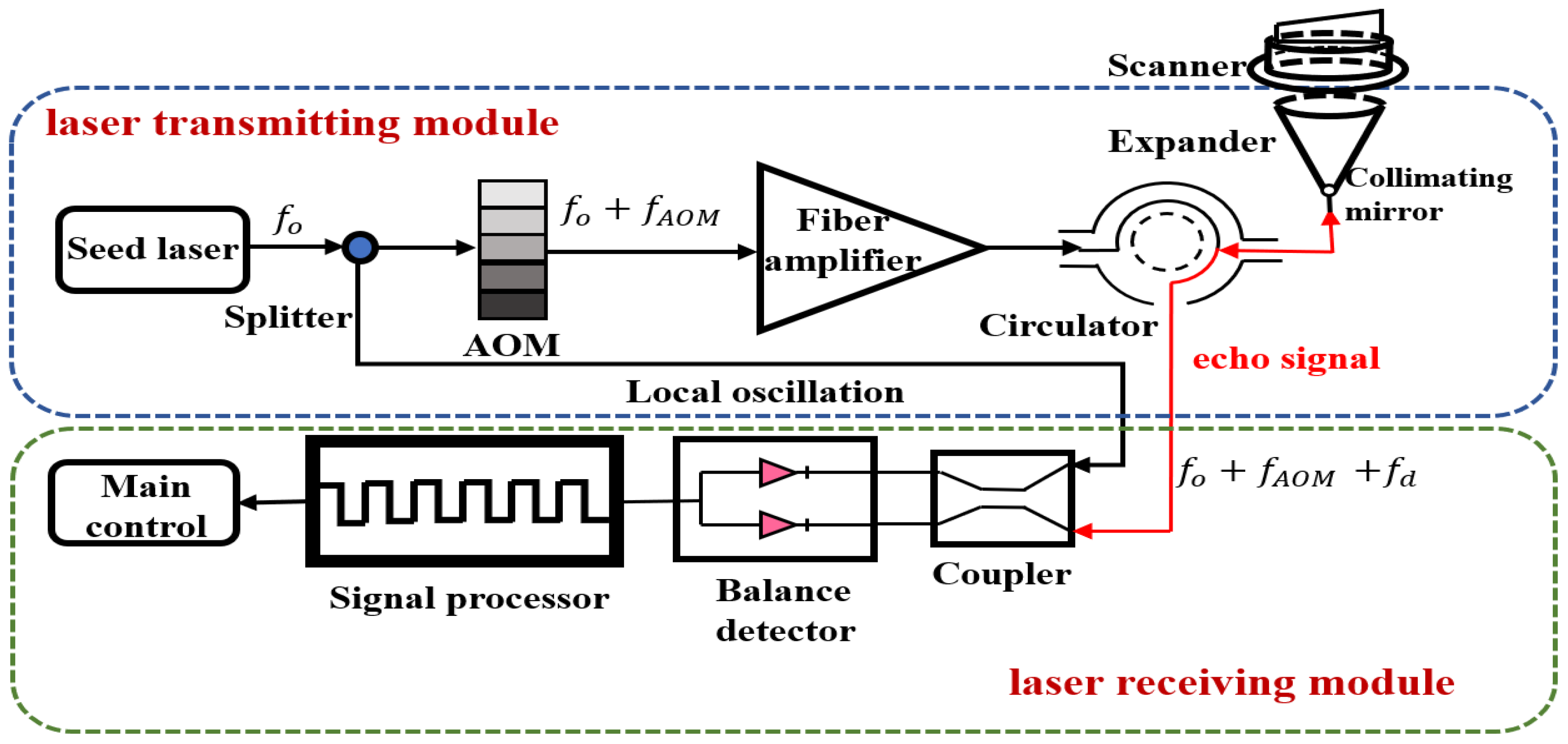
2.1. CDL System

The schematic diagram of the CDL system used in this study is shown in Figure 1. This CDL system consists of a laser transmitter module and a laser receiver module. The laser transmitter module uses a seed source to generate linearly polarized light with a center frequency of ${\mathrm{f}}_0$, which is divided into a transmit signal and a main oscillator signal. The transmit signal is modulated into optical pulses, amplified, and sent into the atmosphere. Due to the Doppler shift effect, the laser receiver module receives an echo signal with a frequency of ${\mathrm{f}}_0$ + ${\mathrm{f}}_{\mathrm{m}}$ + ${\mathrm{f}}_{\mathrm{d}}$. The echo signal and the main oscillator signal are mixed to produce an IF electrical signal (${\mathrm{f}}_{\mathrm{m}}$ + ${\mathrm{f}}_{\mathrm{d}}$.). After sampling by the acquisition card, the echo signal is divided into multiple continuous range gates in time order. The wind-field inversion module processes the signal to estimate the power spectrum, extract the Doppler shifts in different radial directions, and synthesize the 3D atmospheric wind-field information [20,21].

In this study, we used a pulsed CDL system (model KC-WL-2006) manufactured by Hefei Tainuo Lidar Hi-Tech Ltd. in China. The technical parameters of the system are shown in

Table 1. CDL system parameters.

Component	Qualification	Specification
Transmitter	Wavelength	1550 nm
	Pulse energy	145 μJ
	Pulse repetition	10 kHz
	Pulse width	400 ns
Transceiver	Laser mode	Pulse
	Scan mode	Conical
	Elevation angle	60°
	Start angle	0°
	Step angle	90°
Data Acquisition	Sampling frequency	1 GHz
	Sampling points	400
	Range resolution	60 m
	Blind range	60 m
	Gate number	128

. The system adopts pulse triggering mode, with a center frequency of 80 MHz, a wavelength of 1550 nm, a distance resolution of 60 m, and an ideal detection distance of 3000 m. The wind profile measurement chooses the speed azimuth display measurement mode, which has the advantages of high efficiency, relative safety to the human eye, and compact structure [22]. According to the Doppler shift equation, the range of measurable wind speed is ±62 m/s.

2.2. Principle

CDL uses the Doppler principle to detect atmospheric wind speed. By extracting the Doppler shift of the echo signal, wind-speed information can be obtained [23].

The relationship between Doppler shift and radial wind speed is:

$${\mathrm{f}}_{\mathrm{d}}={\mathrm{f}}_{\mathrm{r}}-{\mathrm{f}}_{\mathrm{t}}=\frac{2{\mathrm{V}}_{\mathrm{r}}}{\mathsf{\lambda }}$$

(1)

where ${\mathrm{f}}_{\mathrm{d}}$ is the Doppler shift, ${\mathrm{f}}_{\mathrm{r}}$ is the frequency of the echo signal, ${\mathrm{f}}_{\mathrm{t}}$ is the output laser frequency, ${\mathrm{V}}_{\mathrm{r}}$ is the radial wind speed at which the detected object is moving toward the lidar, and ${\mathrm{V}}_{\mathrm{r}}$ is the wavelength of the laser.

Changes in the wind field of the atmosphere can be depicted through a 3D wind vector [24]. Radial wind speeds are obtained, and the 3D wind vector is synthesized from the four radial wind speeds using vector synthesis. The elevation angle of the lidar is 60°, and the four azimuth angles are 0°, 90°, 180° and 270°, respectively.

3. ANRPR Method

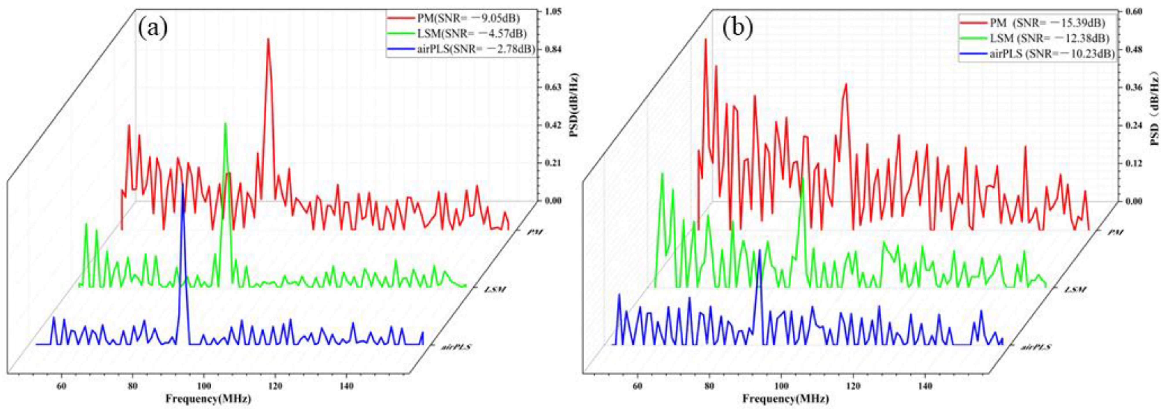
3.1. Existing Method Limitations in Low-SNR Environments

At a low SNR, the extraction of peaks from the echo signal power spectrum becomes biased [24]. The power spectrum image obtained on 29 November 2022 is shown below. The curves in Figure 2a represent the variation of the SNR for different range gates. The SNR gradually decreases as the range gate increases, which leads to a gradual increase in the difficulty of extracting the peaks. Figure 2b shows the spectral data for the 20th range gate, which has a high SNR and can extract the peaks more accurately, and the Doppler shift estimate is unbiased. Figure 2c,d shows the power spectrum data for the 30th and 40th range gates, respectively. The 30th range gate and the 40th range gate have an SNR of −7.5 dB and −15.2 dB, which is low, and the noise floods the peaks, making it difficult to extract the true peaks and bias, so the 3D wind speed synthesized by the vectors is incorrect.

3.2. Division Range Gate

The echo signal received by lidar is converted from the time domain to the frequency domain by FFT to obtain the original signal power spectrum. In wind lidar, to avoid the echo signal being interfered with by noise too far or too close, it is often necessary to divide the echo signal into range gates, i.e., to keep the signal within a certain distance range for subsequent processing [25].

In this study, the pulse width is 400 ns, which corresponds to a distance resolution of $∆\mathrm{R}$ of 60 m. The sampling frequency ${\mathrm{f}}_{\mathrm{s}}$ is 1 GHz, so the number of sampling points for a single range gate is N = 400, and for simplicity of the analysis, the section of the power spectrum that contains the peaks of the valid data is intercepted for analysis. Therefore, each radial in this study was divided into a total of 128 range gates, each storing 112 valid data points, and a total of 14,336 datapoints are collected in each radial for subsequent analysis. The first three range gates represent noise data. The effective power spectrum data are stored in range gates 4 to 128. There is a certain blind spot in lidar ranging, and the height of the blind spot is related to the pulse width, so the detection blind spot B is 60 m. The radial length L of a single range gate can be calculated using the following formula.

$$\mathrm{L}=\frac{\mathrm{c}}{2}\times \frac{\mathrm{N}}{{\mathrm{f}}_{\mathrm{s}}}$$

(2)

Therefore, the length of the nth range gate to the center of the ground is:

$${\mathrm{L}}_{\mathrm{n}}=\mathrm{B}+\mathrm{L}\times \left(\mathrm{n}-0.5\right)$$

(3)

The nth range-gate vertical center height is related to the light-wedge deflection angle $\mathsf{\theta }$. In this study, the light-wedge deflection angle $\mathsf{\theta }$ is 30°, so the nth range-gate vertical center height is:

$${\mathrm{L}}_{\mathrm{v}}={\mathrm{L}}_{\mathrm{n}}\times \cos \mathsf{\theta }$$

(4)

3.3. Range-Gate Noise Removal

Traditional approaches often employ techniques such as PM or LSM to mitigate signal background noise. However, in scenarios characterized by high range gates or low SNR, these conventional methods exhibit suboptimal denoising performance and susceptibility to signal distortion issues. In this study, the power spectral baseline within each range gate is fitted by airPLS, and the fitted curves are used as the noise baseline for that range gate. This process aids the calculation of baseline weights relative to the original signal and controls the smoothing of the baseline with a penalty term, compared to traditional PM and LSM. Each step of the adaptive iterative reweighting process involves solving a weighted penalized least-squares problem of the form:

$${\mathrm{Q}}^{\mathrm{t}}=\sum _{\mathrm{i}=1}^{\mathrm{m}}{\mathrm{w}}_{\mathrm{i}}^{\mathrm{t}}|{\mathrm{x}}_{\mathrm{i}}-{\mathrm{z}}_{\mathrm{i}}^{\mathrm{t}}{|}^2+\mathsf{\lambda }\sum _{\mathrm{j}=2}^{\mathrm{m}}|{\mathrm{z}}_{\mathrm{j}}^{\mathrm{t}}-{\mathrm{z}}_{\mathrm{j}-1}^{\mathrm{t}}{|}^2$$

(5)

where $\mathrm{x}$ is the signal vector, $\mathrm{z}$ is the fitting vector and $\mathrm{w}$ is the weight vector obtained by adaptive iterative method. At the start step, we initialize ${\mathrm{w}}^0$ = 1. After initialization, $\mathrm{w}$ for each iteration step $\mathrm{t}$ is obtained using the following expression:

The vector consists of the difference between $\mathrm{x}$ and ${\mathrm{z}}^{\mathrm{t}-1}$ during the iteration step of $\mathrm{t}$. The iteration will stop with the maximum number of iterations or when the termination condition is reached. The iteration will stop with the maximum number of iterations or when the termination condition is reached. The termination conditions are as follows:

$$\left|{\mathrm{d}}_{\mathrm{t}}\right|<0.001\times \left|\mathrm{x}\right|$$

(6)

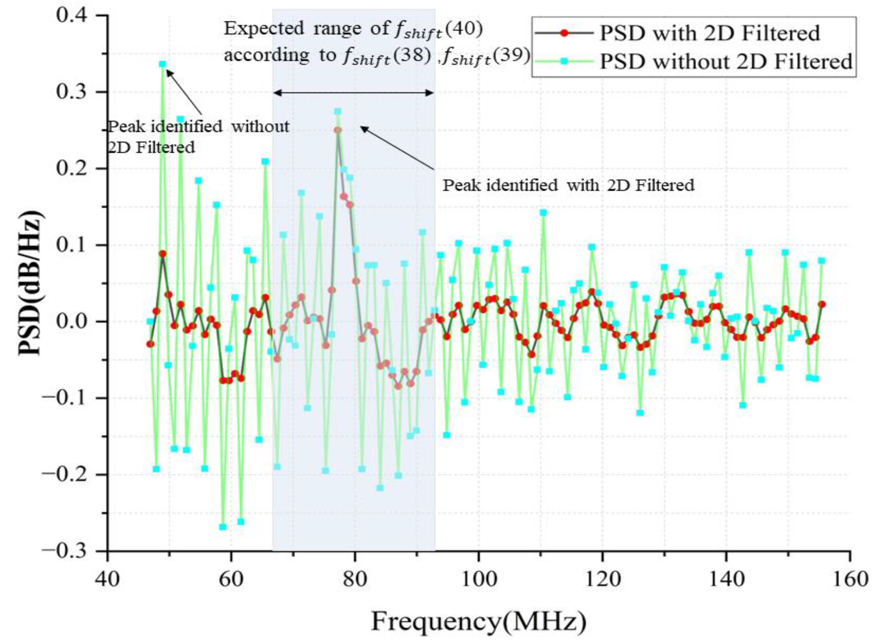
3.4. 2D Gaussian Filter

With a resolution of only a few tens of meters, the wind measurement lidar is smaller than most wind shear [26]. Based on the spatial continuity of wind speeds in a smooth atmosphere, it is unlikely that wind speeds at adjacent distance doors will change significantly [19]. Thus, according to this characteristic of the wind field, 2D low-pass Gaussian filtering is used to enhance the correlation between the range gates, and then the peak extraction is carried out, which effectively reduces the influence of the peak extraction by the noise and improves the accuracy of the extracted peaks. The size of the filter ${\mathrm{H}}_{\mathrm{G}}$ used is $\mathrm{l}\times \mathrm{l}(\mathrm{l}=2\mathrm{a}+1,\mathrm{a}=1,2,\dots )$. Where ${\mathrm{PSD}}_{\mathrm{raw}}$ is the 2D power spectrum data, ${\mathrm{PSD}}_{\mathrm{G}}$ is the Gaussian-filtered PSD.

$$\left\{\begin{array}{c}{\mathrm{H}}_{\mathrm{G}}=\frac{1}{2\mathsf{\pi }{\mathsf{\sigma }}_{\mathrm{H}}^2}\exp \left[-\frac{{\left(\mathrm{s}-\mathrm{a}\right)}^2+{\left(\mathrm{t}-\mathrm{a}\right)}^2}{2{\mathsf{\sigma }}_{\mathrm{H}}^2}\right]\\ {\mathrm{PSD}}_{\mathrm{G}}={\mathrm{H}}_{\mathrm{G}}\times {\mathrm{PSD}}_{\mathrm{raw}}\end{array}\right.,\mathrm{s},\mathrm{t}=0,1,\dots \mathrm{l}-1$$

(7)

3.5. Adaptive Peak-Retrieval Algorithm

In the echo power spectrum, the Doppler shift due to scattering motion in the lidar beam is determined by identifying the highest value in the power spectrum [27]. The adaptive peak-retrieval algorithm is a method for automatic peak detection of noisy periodic and quasi-periodic signals based on the multi-scale automatic peak-retrieval algorithm and optimized for the power spectral characteristics of coherent wind measurement lidar echo signals. Compared to the traditional peak extraction algorithm, the adaptive peak-retrieval algorithm has the advantages of high efficiency and does not require any free parameters [28].

Firstly, the local maxima scalogram (LMS) $\mathrm{M}$ of the data series is established. The cumulative spectra were transformed into a long sequence $\mathrm{X}$, ${\mathrm{X}=[\mathrm{x}}_1,{\mathrm{x}}_2,\dots ,{\mathrm{x}}_{\mathrm{n}}$], n = 14,336.

The local maximum of the signal $X$ is determined using the moving window method, where the length of the window $w_k$ is varied {${\mathrm{w}}_{\mathrm{k}}=2\mathrm{k}|\mathrm{k}=1,2,\dots ,\mathrm{L}$}, Comp are the value of each data point in the sequence with the values of the leading and trailing edge points in the range, the logical values of the comparisons are used as the fluctuation factors, and the fluctuation factors are used as data elements to create the matrix $\mathrm{M}(\mathrm{n}\times \mathrm{m})$, where $m=[\mathrm{n}/2]-1$. $\left[\mathrm{z}\right]$ is a downward rounding function. For each dimension, $k$ and $\mathrm{i}(1\le \mathrm{i}\le \mathrm{n})$, ${\mathrm{m}}_{\mathrm{k},\mathrm{i}}$ can be expressed as

$${\mathrm{m}}_{\mathrm{k},\mathrm{i}}=\left\{\begin{array}{l}0,\left({\mathrm{x}}_{\mathrm{i}}>{\mathrm{x}}_{\mathrm{i}-\mathrm{k}}\cap {\mathrm{x}}_{\mathrm{i}}>{\mathrm{x}}_{\mathrm{i}+\mathrm{k}}\right)\\ 1,\mathrm{otherwise}\end{array}\right.$$

(8)

The matrix M can be expressed as

$$\mathrm{M}=\left[\begin{array}{ccc}{\mathrm{m}}_{11}& \begin{array}{cc}{\mathrm{m}}_{12}& \cdots \end{array}& {\mathrm{m}}_{1\mathrm{n}}\\ {\mathrm{m}}_{21}& \begin{array}{cc}{\mathrm{m}}_{22}& \cdots \end{array}& {\mathrm{m}}_{2\mathrm{n}}\\ \begin{array}{c}⋮\\ {\mathrm{m}}_{\mathrm{n}1}\end{array}& \begin{array}{c}\begin{array}{cc}⋮& \ddots \end{array}\\ \begin{array}{cc}{\mathrm{m}}_{\mathrm{n}2}& \cdots \end{array}\end{array}& \begin{array}{c}⋮\\ {\mathrm{m}}_{\mathrm{nn}}\end{array}\end{array}\right]$$

(9)

The presence or absence of a zero element in matrix $\mathrm{M}$ determines if there is a maximum value in the spectral data sequence within range $\mathrm{N}$. The matrix’s zero element is responsible for the determination of the maximum value in range $\mathrm{N}$.

The matrix is then row-summed to find the row $\mathsf{\gamma }$ with the smallest row-sum value. The rows with $\mathrm{k}>\mathsf{\gamma }$ in the local maximum matrix are deleted to construct a new matrix ${\mathrm{M}}_{\mathrm{r}}{(\mathrm{m}}_{\mathrm{k},\mathrm{i}})$ where $\mathrm{i}=\{1,2\dots ,\mathrm{n}\}$, $\mathrm{k}=\{1,2\dots ,$ $\mathsf{\gamma }\}$. Finally, a column summation is performed on the new matrix, and if the column summation value is zero, then the index value of the column is classified as a peak.

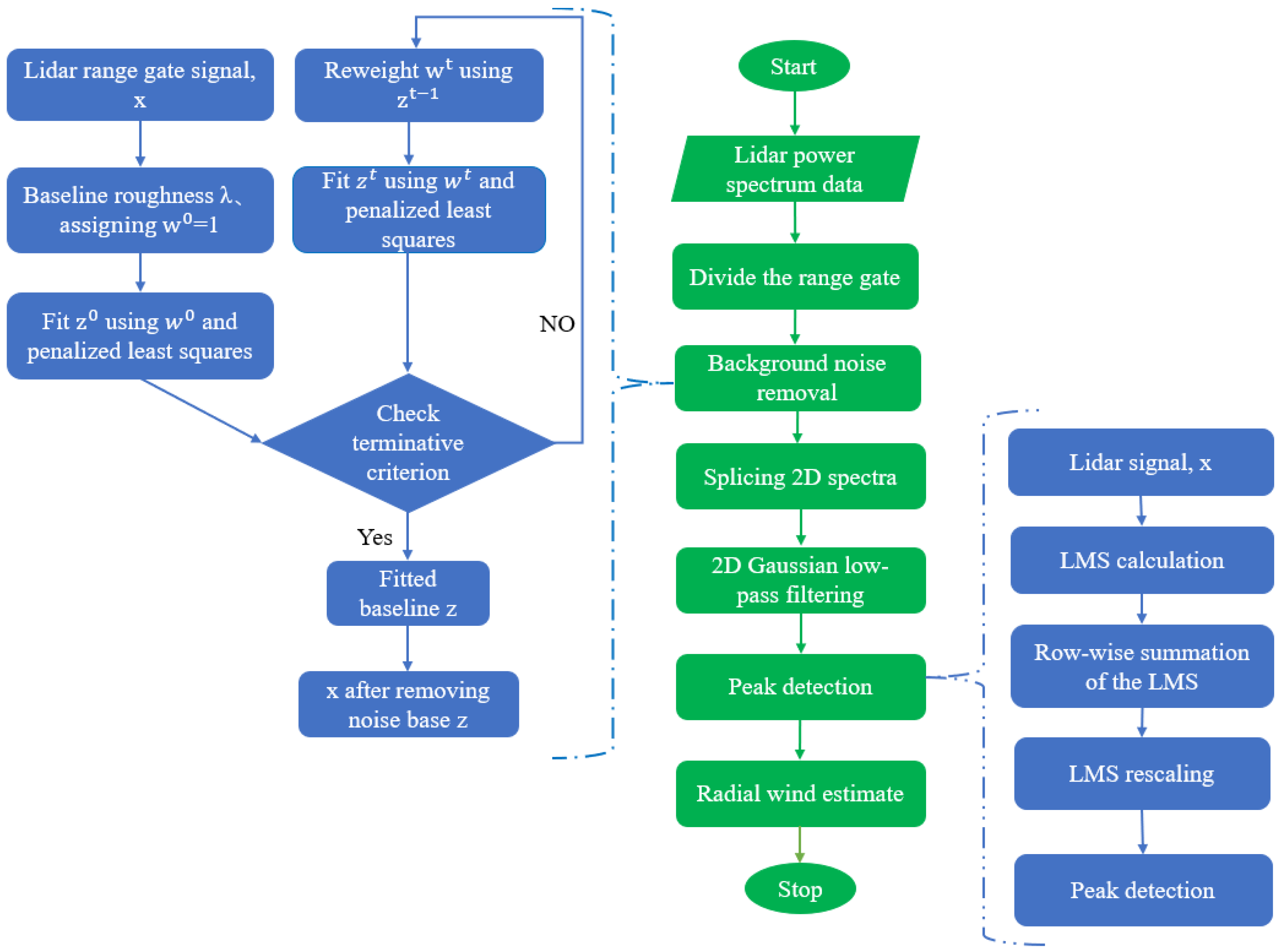
3.6. Design Procedure for ANRPR

The detailed steps of the noise-reduction-based peak-retrieval algorithm are as follows:

• Substrate noise removal: The raw data for each range gate are subjected to adaptive iterative weighted penalized least-squares fitting, and the corresponding noise-substrate removal is performed for each range gate to obtain the power spectral data after the removal of background noise.
• Spectrum signal splicing: The power spectrum data with background noise removed are arranged radially by a range gate to form a 2D matrix spectrum.
• 2D Gaussian low-pass filtering: The 2D spectral matrix is subjected to 2D Gaussian low-pass filtering to improve the correlation of the range gates.
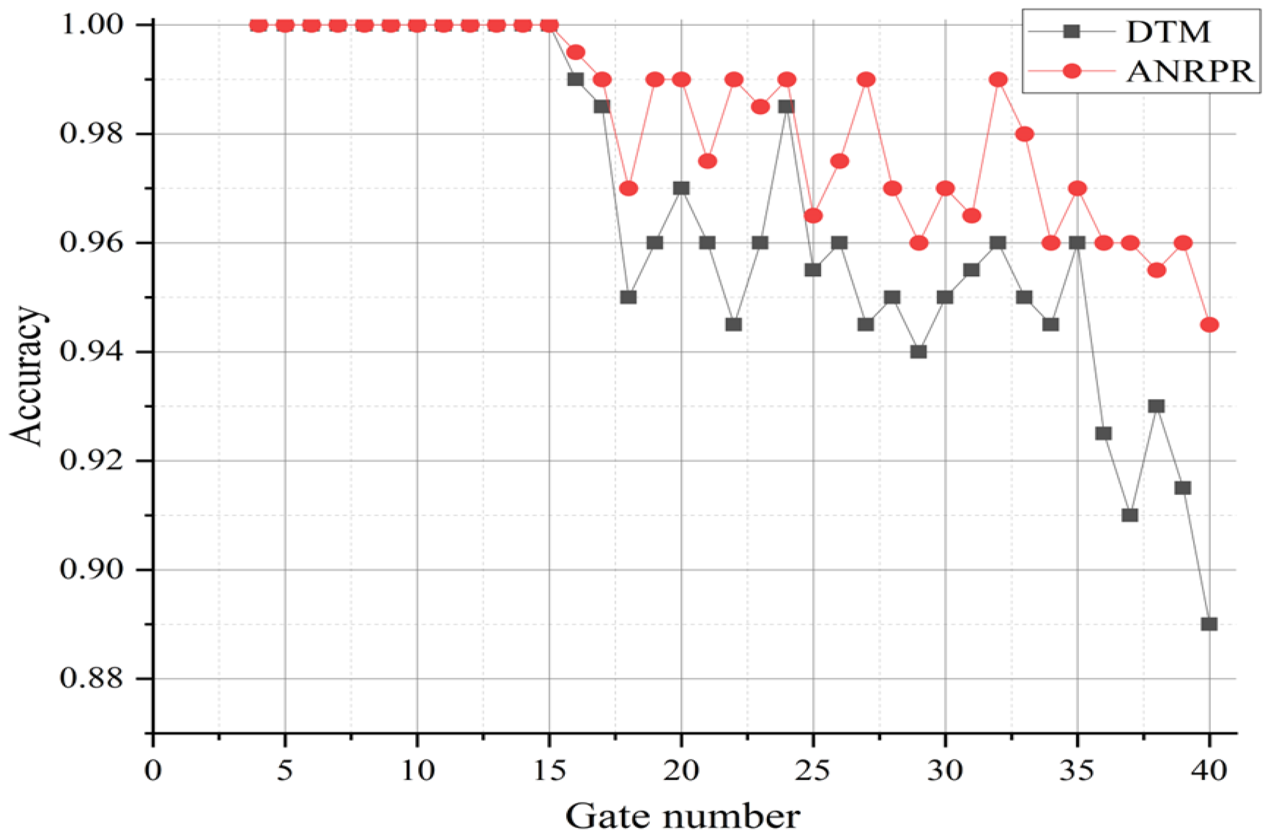
• Peak search: The filtered 2D spectral matrix is expanded by range gates to obtain the noise-reduced 1D power spectral data, and the peaks of each range gate are extracted using a peak-retrieval algorithm.
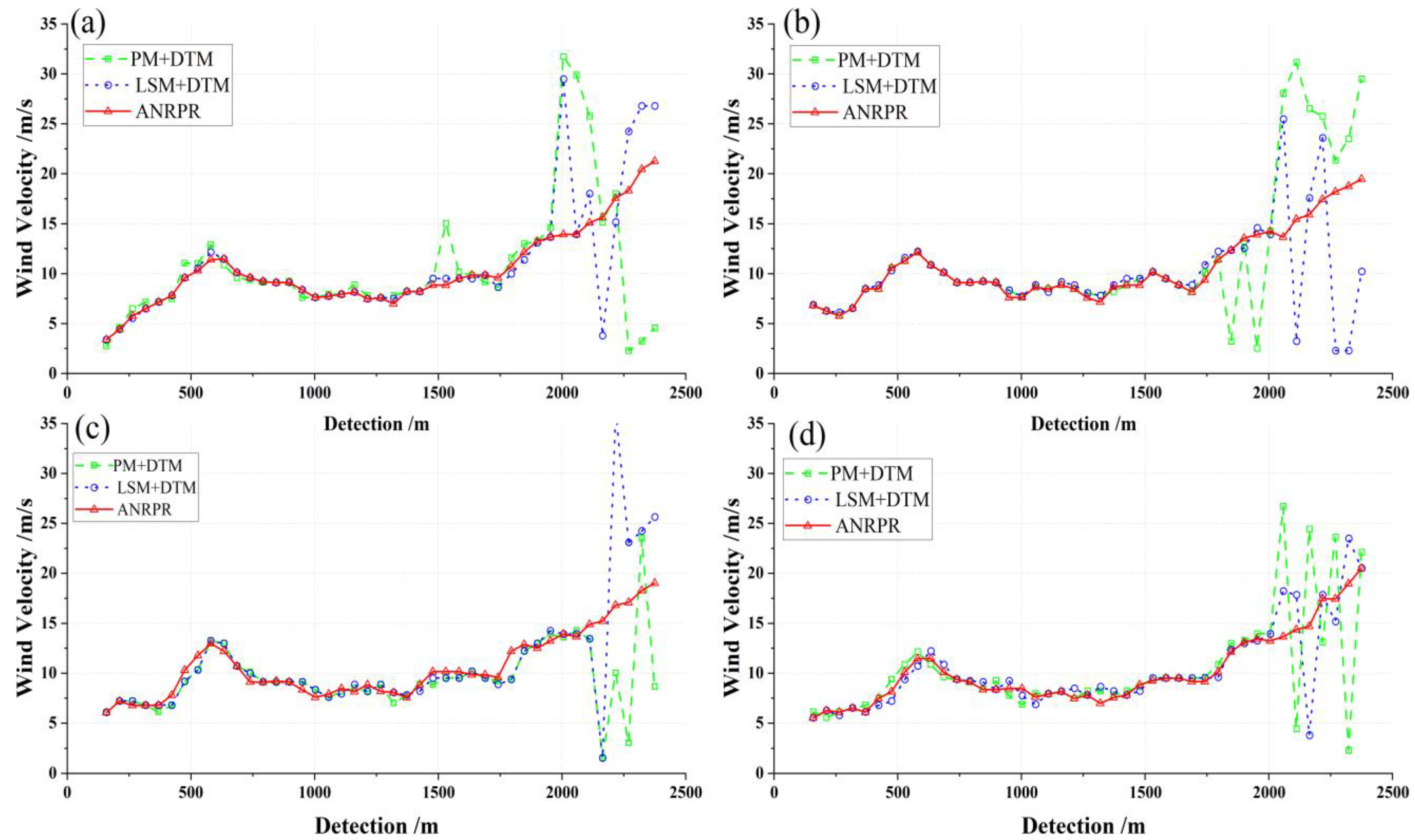
• Estimation of radial wind speed: For each distance gate retrieved peak, its corresponding frequency and the radial wind speed are found by the Doppler shift formula.

The algorithm’s process is illustrated in Figure 3.

Table 2. Comparison table between ANRPR and different existing algorithms.

Method	Application Of Lidar Data	Noise Reduction	Peak Retrieval
PM [12]	$\surd$	$\surd$	$\times$
LSM [13]	$\surd$	$\surd$	$\times$
DTM [16]	$\surd$	$\times$	$\surd$
DCM [15]	$\surd$	$\times$	$\surd$
ANRPR	$\surd$	$\surd$	$\surd$

shows the comparison table of the existing methods. In this table, $\surd$ indicates applicability, $\times$ indicates inapplicability. In the experiments of this study, we will verify the advantages of the ANRPR algorithm in terms of detection distance as well as detection accuracy by comparing the combination of the above traditional methods. Figure 4 shows radial wind speeds in four different directions; the red curve represents the radial wind speed with ANRPR (new method) and the blue curve represents the radial wind speed with conventional background noise removal plus the conventional peak-finding method (old method). The SNR of the lidar data decreases as the detection area of the lidar increases, as can be seen in the figure in the first few range gates, i.e., the high-SNR portion of the two methods is almost identical. As the range gates increase, the old method gradually shows some deviations from the values, which seriously deviate from the spatial continuity of the wind speed, and in some cases, the absolute difference between the neighboring range gates is more than 10 m/s. This is shown in Figure 4 at the 24th point from the door and the 43rd point from the door. The ANRPR algorithm significantly improves the continuity of the wind speed and reduces the probability of outliers, which is in line with the actual situation of the minimum oscillation of the wind field in the wind field.

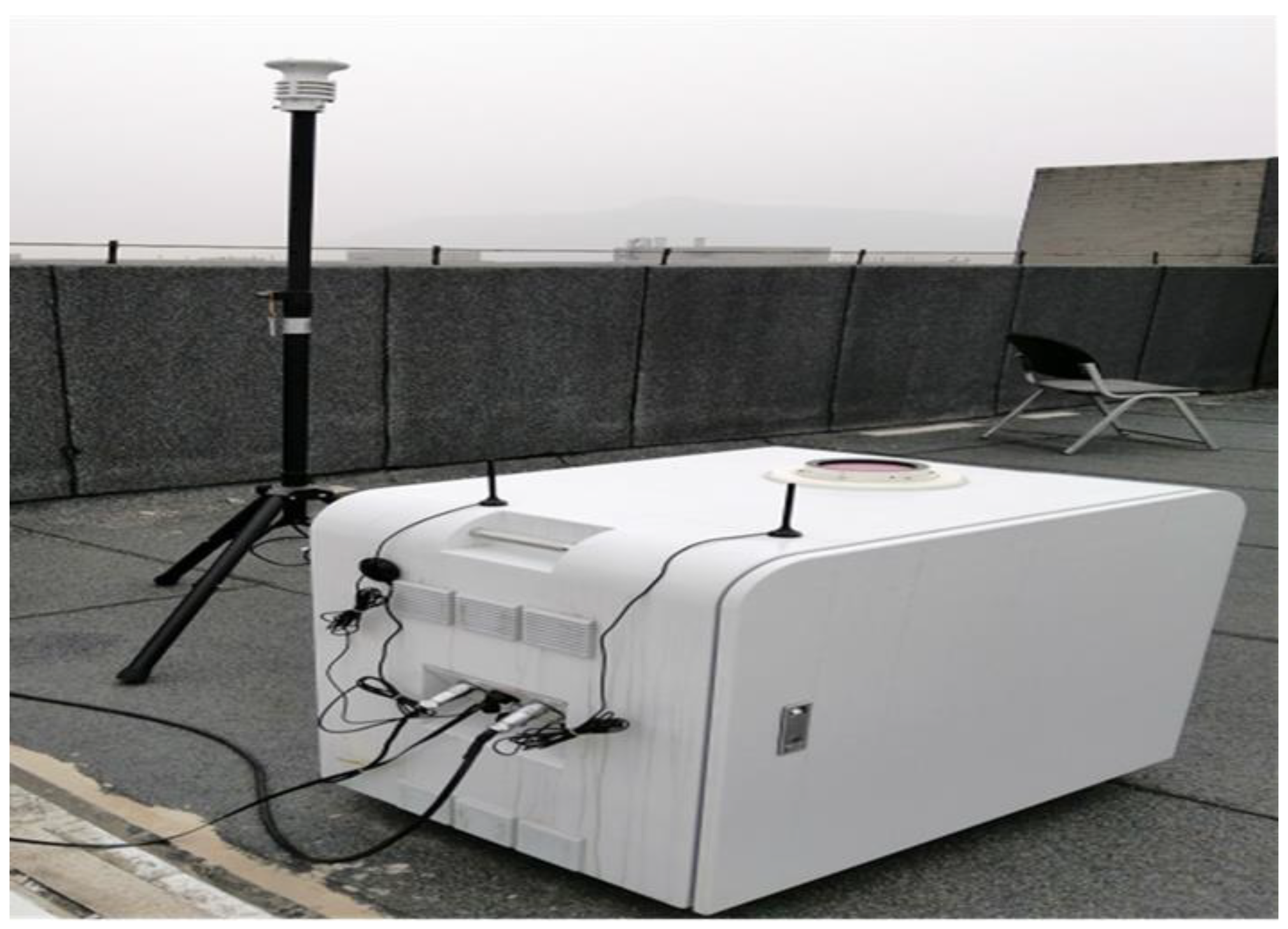
4. Experimental Results and Discussion

In order to validate the effectiveness of the ANRPR algorithm, observational experiments were conducted on 27 November 2022 using the available lidar, as shown in Figure 5. The experimental site is at Shandong Normal University, Changqing District, Jinan City, Shandong Province, China (36.5° N, 116.8° E). The time-domain data are collected using a 500 MHz sampling frequency acquisition board, and the spectrum of each pulse is summed and averaged, then inverted in the time domain and compressed into a single signal. The power spectrum of the frequency domain signal is obtained by FFT, and the peak of the power spectrum is extracted to calculate the radial wind speed.

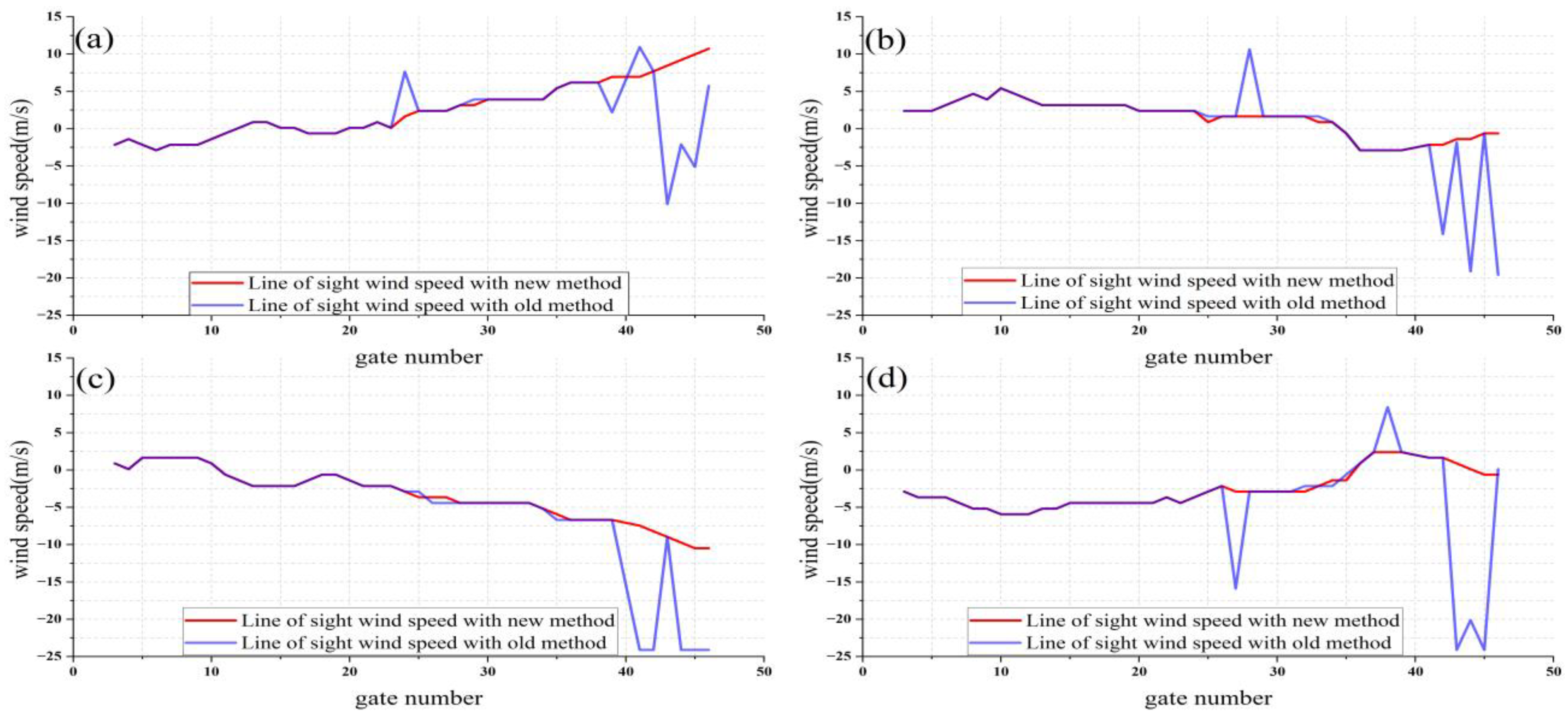
4.1. ANRPR Algorithm Analysis

The ANRPR algorithm involves background removal, filtering, and peak retrieval. In terms of background removal, comparisons are made by airPLS with the periodogram method and the least-squares polynomial fitting method by processing real data.

Figure 6 shows the power spectrum data for the second line of sight (90° direction) at 08:00 on 29 November 2022 for two different range gates after background denoising. The data, which contain some negative values, are adjusted by setting any negative values to zero. Figure 6a presents the 35th range-gate power spectrum data point, and Figure 6b displays the 40th range-gate power spectrum data point. In Figure 6a, it is evident that all three methods excel in background noise reduction, resulting in significantly enhanced peak visibility with a notable increase in SNR. However, with the increasing detection distance and the influence of atmospheric turbulence, a large amount of noise is introduced, and the peaks are drowned out by the noise. In Figure 6b, the background noise is removed by the PM method, and the noise peaks are obviously higher than the signal peaks, while the signal peaks after the LSM method are not obviously prominent, and the power spectrum data after the airPLS method are processed and the signal peaks are obviously visible. Additionally, the SNR of the processed power spectral data using the airPLS method demonstrate an increase from −12.38 dB to −10.23 dB when compared to the LSM method. Therefore, the results demonstrate that, compared to the LSM and PM methods, the airPLS method is more effective in reducing background noise and improving SNR.

Moreover, 2D low-pass filtering reduces small fluctuations in the signal and increases the continuity of the front-to-back range gates. Figure 7 shows a comparison of the 40th range-gate power spectrum data point before and after the 2D filtering operation. Based on the 38th and 39th range gates, it was able to deduce that the signal peak should be in the shaded region; however, the noise at 48 MHz clearly exceeds the peak of the signal, making it an incorrect signal peak and thus an incorrect estimate of the radial wind. The correct peaks can be found by 2D filtering, exploiting the spatial continuity of the atmospheric wind field.

In this study, a representative sample of 200 known detected wind-speed power spectrum data items are selected and analyzed, as shown in Figure 8; firstly, they are subjected to background noise removal and filtering, and then they are tested for accuracy using ANRPR and DTM, respectively. This study performed peak searches for the first 40 range gates of each power spectrum data point, and we were able to find that the accuracy of peak-finding gradually decreased as the range gates increased. In particular, when using the traditional derivative thresholding method, it is easy to obtain incorrect peak information at a low SNR; on the contrary, the adaptive peak-retrieval algorithm has better robustness and accuracy in the peak-finding of wind lidar power spectrum data compared to traditional algorithms.

4.2. Wind-Field Inversion Based on ANRPR Method

The panoramic display of continuously observed wind profiles eases the understanding of trends in the wind field and validates analyses. A comparison of the results of the wind profiles is conducted by graphs, since the validation shows the advantages of each algorithm. The horizontal wind-speed profiles after ANRPR and PM+DTM and LSM+DTM treatments are shown in Figure 9. Four datasets, recorded at 01:00, 01:15, 01:30, and 01:45 on the 29th day, were chosen for comparison. The altitude range of 0 to 2.5 km was selected for analysis.

As shown in Figure 9, the magnitude of the wind speeds of the three algorithms is relatively coincident at heights below 1.5 km, and the three methods are similar. However, for the PM, it starts to fluctuate at 1.5 km and the wind-speed error between neighboring range gates gradually increases, and the accuracy of wind-speed estimation is greatly reduced; at 2 km, the wind speed estimated by the LSM starts to deteriorate, and the spatial continuity of wind speed is no longer maintained. The wind speed estimated with the adaptive noise-reduction peak-retrieval algorithm remains at the same level above 2 km. By comparing the three methods mentioned above, the farthest detection ranges for wind-speed estimation are 1.6 km, 2.1 km, and 2.4 km, respectively. There are small abrupt changes in wind speeds in Figure 9, indicating fluctuating wind speeds, which are frequent, with significant contrast as the detection distance increases or the SNR decreases. The ANRPR algorithm performs best compared to the other two methods.

The ANRPR algorithm can also be used for wind-speed estimation on large amounts of continuously observed wind lidar data as it will return a reasonable peak and retrieve the location efficiently and accurately, especially at a low SNR.

As the SNR decreases over a long acquisition period, the number of poor estimates of wind speed increases because the signal is sometimes lost in the noise and cannot be extracted, making it impossible to invert the true wind speed, as shown in red and black in Figure 10 and Figure 11. In contrast, the wind speeds inverted by the ANRPR algorithm exhibit good continuity in spatial and temporal distribution as well as in stratification, showing the best stability with the least number of poor estimates. To quantitatively compare the three aforementioned methods, the 15 min wind-speed data are evaluated as a whole. This evaluation involves calculating the cumulative means of the horizontal and vertical wind-speed values in the time dimension, along with their respective standard errors.

As shown in Figure 10d and Figure 11d, after averaging 30 sets of vertical and horizontal wind-speed time series data, it is evident that the three different noise-reduction peak search algorithms employed present almost identical wind-speed distributions over a range of 1.25 km. However, beyond this point, a notable divergence is observed. Due to the stability of the atmosphere, the size of wind speed in the vertical direction is very small; it is almost zero. From the figure, we can observe that the magnitude of the vertical wind speed of the new algorithm fluctuates between 0 and −1 within 2.5 km, and the standard error is also within ±0.5 m/s, which is within the permissible range of wind-speed accuracy. The standard error gradually increases with increasing height, which is due to the fact that the signal strength decreases with distance and the SNR gradually decreases, increasing the error rate of peak-finding. For horizontal wind speed, the total standard errors of the three methods for all range gates within the detection range are 5.71 m/s, 19.53 m/s, and 27.28 m/s, respectively. Compared to the other two algorithms, the new algorithm estimated speeds, with smaller standard errors and improved detection distance, by 26.3% and 85.1%, respectively. Therefore, the ANRPR algorithm improves wind-speed estimation and increases the accuracy and detection distance of wind-speed estimation.

Based on meteorological data obtained from the Jinan Meteorological Bureau on November 29th, it was observed that on that particular night, near-surface winds reached levels 4 to 5. These wind levels correspond to horizontal near-surface wind speeds in the range of approximately 5.5 to 10.7 m per second. With increasing altitude, the influence of ground friction diminishes, resulting in a gradual increase in wind speed. However, during this period, a gradual reduction in wind speed was observed between altitudes of 0.5 km and 1.25 km. This phenomenon is likely attributable to localized air currents within the mountainous region, leading to the gradual reduction in wind speed within this specific altitude range.

To comprehensively evaluate the ANRPR algorithm’s performance under low-SNR conditions, Figure 12 presents the comparative analysis of the three methods applied to the 40th range gate over continuous time. Typically, atmospheric wind fields exhibit gradual changes over time. The figure highlights that the ANRPR algorithm demonstrates superior stability in continuous time performance, in contrast to the other two methods, which exhibit significant fluctuations and unstable inversion results at lower SNR levels. This observation suggests that the ANRPR algorithm exhibits enhanced adaptability within atmospheric wind fields under low-SNR scenarios, delivering more stable and accurate wind-speed inversion results.

To further validate the stability of the ANRPR algorithm, we analyzed the horizontal wind speed and horizontal wind direction of the above three methods for correlation and comparison with standard data at different heights of the meteorological gradient tower. We selected lidar data for 23 June 2023, averaged the horizontal wind speed and horizontal wind direction at 10 min intervals, and compared them with the meteorological gradient tower wind-speed data. As shown in

Table 3. Correlation of horizontal wind speed and direction with meteorological gradient tower data at different heights.

Height(m)	Horizontal Wind Velocity Correlation Based on ANRPR	Horizontal Wind Velocity Correlation Based on LSM+DTM	Horizontal Wind Velocity Correlation Based on PM+DTM	Horizontal Wind Direction Correlation Based on ANRPR	Horizontal Wind Direction Correlation Based on LSM+DTM	Horizontal Wind Direction Correlation Based on PM+DTM
150	0.9556	0.9442	0.9202	0.9514	0.9410	0.9257
200	0.9458	0.9332	0.9174	0.9421	0.9356	0.9210
250	0.9302	0.9101	0.8921	0.9287	0.9241	0.9142
300	0.9278	0.9076	0.8842	0.9217	0.9102	0.8987
350	0.9203	0.8962	0.8729	0.9129	0.8981	0.8845

:

From the above table, it can be found that the horizontal wind speed and direction using the ANRPR algorithm are in good agreement with the data from the meteorological gradient tower, and the correlation coefficients are consistently above 0.9 in these height ranges. It can be seen that compared to the other two algorithms, ANRPR has higher accuracy and stability of performance in the case of long-time detection.

5. Conclusions

Traditional noise-reduction peak-retrieval algorithms often exhibit instability under low-SNR conditions. Addressing this issue, this study proposes a fast and effective Doppler peak-estimation algorithm for wind profiles (ANRPR). It not only efficiently applies to wind profile data processing under low-SNR conditions but also eliminates the need for artificially setting free parameters in peak retrieval. Experimental comparisons with two traditional algorithms show improvements in detection distance by 26.3% and 85.1%, respectively, with a longer detection distance. In terms of accuracy, correlation comparisons with wind-field information from a meteorological gradient tower yield a correlation coefficient of 0.95, indicating higher detection accuracy and reliability. The algorithm finds applications not only in fixed-end Doppler lidar for atmospheric wind-field detection but also in vehicle-mobile settings for accurate on-the-move detection. Future research aims to further study and enhance the algorithm for a wider range of practical application scenarios.

References

1. Kotake, N.; Sakamaki, H.; Imaki, M.; Miwa, Y.; Ando, T.; Yabugaki, Y.; Enjo, M.; Kameyama, S. Intelligent and compact coherent Doppler lidar with fiber-based configuration for robust wind sensing in various atmospheric and environmental conditions. Opt. Express 2022, 30, 20038–20062. [Google Scholar] [CrossRef] [PubMed]
2. Shangguan, M.; Xia, H.; Wang, C.; Qiu, J.; Shentu, G.; Zhang, Q.; Dou, X.; Pan, J.W. All-fiber upconversion high spectral resolution wind lidar using a Fabry-Perot interferometer. Opt. Express 2016, 24, 19322–19336. [Google Scholar] [CrossRef] [PubMed]
3. Xia, H.; Shentu, G.; Shangguan, M.; Xia, X.; Jia, X.; Wang, C.; Zhang, J.; Pelc, J.S.; Fejer, M.M.; Zhang, Q.; et al. Long-range micro-pulse aerosol lidar at 1.5 mum with an upconversion single-photon detector. Opt. Lett. 2015, 40, 1579–1582. [Google Scholar] [CrossRef] [PubMed]
4. Böhme, G.S.; Fadigas, E.A.; Martinez, J.R.; Tassinari, C.E.M. Analysis of the Use of Remote Sensing Measurements for Developing Wind Power Projects. J. Sol. Energy Eng. 2019, 141, 41005. [Google Scholar] [CrossRef]
5. Yang, Y.J.; Yim, S.H.L.; Haywood, J.; Osborne, M.; Chan, J.C.S.; Zeng, Z.L.; Cheng, J.C.H. Characteristics of Heavy Particulate Matter Pollution Events Over Hong Kong and Their Relationships With Vertical Wind Profiles Using High-Time-Resolution Doppler Lidar Measurements. J. Geophys. Res.-Atmos. 2019, 124, 9609–9623. [Google Scholar] [CrossRef]
6. Chen, X.; Dai, G.; Wu, S.; Liu, J.; Yin, B.; Wang, Q.; Zhang, Z.; Qin, S.; Wang, X. Coherent high-spectral-resolution lidar for the measurement of the atmospheric Mie-Rayleigh-Brillouin backscatter spectrum. Opt. Express 2022, 30, 38060–38076. [Google Scholar] [CrossRef] [PubMed]
7. Diao, W.F.; Zhang, X.; Liu, J.Q.; Zhu, X.P.; Liu, Y.; Bi, D.C.; Chen, W.B. All fiber pulsed coherent lidar development for wind profiles measurements in boundary layers. Chin. Opt. Lett. 2014, 12, 72801. [Google Scholar] [CrossRef]
8. Gottschall, J.; Gribben, B.; Stein, D.; Würth, I. Floating lidar as an advanced offshore wind speed measurement technique: Current technology status and gap analysis in regard to full maturity. Wiley Interdiscip. Rev.-Energy Environ. 2017, 6, e250. [Google Scholar] [CrossRef]
9. Chumchean, S.; Sharma, A.; Seed, A. Radar rainfall error variance and its impact on radar rainfall calibration. Phys. Chem. Earth Parts A/B/C 2003, 28, 27–39. [Google Scholar] [CrossRef]
10. Karlsson, C.J.; Olsson, F.; Letalick, D.; Harris, M. All-fiber multifunction continuous-wave coherent laser radar at 1.55 μm for range, speed, vibration, and wind measurements. Appl. Opt. 2000, 39, 3716–3726. [Google Scholar] [CrossRef]
11. Pearson, G.N.; Roberts, P.J.; Eacock, J.R.; Harris, M. Analysis of the performance of a coherent pulsed fiber lidar for aerosol backscatter applications. Appl. Opt. 2002, 41, 6442–6450. [Google Scholar] [CrossRef] [PubMed]
12. Beyon, J.Y.; Koch, G.J. Novel nonlinear adaptive Doppler-shift estimation technique for the coherent Doppler validation lidar. Opt. Eng. 2007, 46, 16002. [Google Scholar] [CrossRef]
13. Bu, Z.C.; Zhang, Y.C.; Chen, S.Y.; Guo, P.; Li, L.; Chen, H. Noise modeling by the trend of each range gate for coherent Doppler LIDAR. Opt. Eng. 2014, 53, 63109. [Google Scholar] [CrossRef]
14. Wu, Y.; Guo, P.; Chen, S.; Chen, H.; Zhang, Y. Wind profiling for a coherent wind Doppler lidar by an auto-adaptive background subtraction approach. Appl. Opt. 2017, 56, 2705–2713. [Google Scholar] [CrossRef] [PubMed]
15. Jarman, K.H.; Daly, D.S.; Anderson, K.K.; Wahl, K.L. A new approach to automated peak detection. Chemom. Intell. Lab. Syst. 2003, 69, 61–76. [Google Scholar] [CrossRef]
16. Yin, W.H.; Huang, R.; Qi, R.J.; Duan, C.A. Extraction of Structural and Chemical Information from High Angle Annular Dark-Field Image by an Improved Peaks Finding Method. Microsc. Res. Tech. 2016, 79, 820–826. [Google Scholar] [CrossRef] [PubMed]
17. Rabbani, H.; Mahjoob, M.; Farahabadi, E.; Farahabadi, A. R peak detection in electrocardiogram signal based on an optimal combination of wavelet transform, Hilbert transform, and adaptive thresholding. J. Med. Signals Sens. 2011, 1, 91. [Google Scholar] [CrossRef] [PubMed]
18. Liu, H.; Hu, F.; Su, J.S.; Wei, X.W.; Qin, R.S. Comparisons on Kalman-Filter-Based Dynamic State Estimation Algorithms of Power Systems. IEEE Access 2020, 8, 51035–51043. [Google Scholar] [CrossRef]
19. Lin, R.; Guo, P.; Chen, H.; Chen, S.; Zhang, Y. Smoothed accumulated spectra based wDSWF method for real-time wind vector estimation of pulsed coherent Doppler lidar. Opt. Express 2022, 30, 180–194. [Google Scholar] [CrossRef]
20. Wu, S.; Liu, B.; Liu, J.; Zhai, X.; Feng, C.; Wang, G.; Zhang, H.; Yin, J.; Wang, X.; Li, R.; et al. Wind turbine wake visualization and characteristics analysis by Doppler lidar. Opt. Express 2016, 24, A762–A780. [Google Scholar] [CrossRef]
21. Kameyama, S.; Ando, T.; Asaka, K.; Hirano, Y.; Wadaka, S. Performance of Discrete-Fourier-Transform-Based Velocity Estimators for a Wind-Sensing Coherent Doppler Lidar System in the Kolmogorov Turbulence Regime. IEEE Trans. Geosci. Remote Sens. 2009, 47, 3560–3569. [Google Scholar] [CrossRef]
22. Shangguan, M.; Wang, C.; Xia, H.; Shentu, G.; Dou, X.; Zhang, Q.; Pan, J.-W. Brillouin optical time domain reflectometry for fast detection of dynamic strain incorporating double-edge technique. Opt. Commun. 2017, 398, 95–100. [Google Scholar] [CrossRef]
23. Zhao, Y.; Zhang, X.; Zhang, Y.; Ding, J.; Wang, K.; Gao, Y.; Su, R.; Fang, J. Data Processing and Analysis of Eight-Beam Wind Profile Coherent Wind Measurement Lidar. Remote Sens. 2021, 13, 3549. [Google Scholar] [CrossRef]
24. Yuan, J.; Xia, H.; Wei, T.; Wang, L.; Yue, B.; Wu, Y. Identifying cloud, precipitation, windshear, and turbulence by deep analysis of the power spectrum of coherent Doppler wind lidar. Opt. Express 2020, 28, 37406–37418. [Google Scholar] [CrossRef] [PubMed]
25. Banakh, V.A.; Brewer, A.; Pichugina, E.L.; Smalikho, I.N. Measurements of wind velocity and direction with coherent Doppler lidar in conditions of a weak echo signal. Atmos. Ocean. Opt. 2010, 23, 381–388. [Google Scholar] [CrossRef]
26. Sinha, S.; Sarma, T.V.C.; Regeena, M.L. Estimation of Doppler Profile Using Multiparameter Cost Function Method. IEEE Trans. Geosci. Remote Sens. 2017, 55, 932–942. [Google Scholar] [CrossRef]
27. Zhang, X.; Li, Q.; Wang, Y.; Fang, J.; Zhao, Y. Field Verification of Vehicle-Mounted All-Fiber Coherent Wind Measurement Lidar Based on Four-Beam Vertical Azimuth Display Scanning. Remote Sens. 2023, 15, 3377. [Google Scholar] [CrossRef]
28. Scholkmann, F.; Boss, J.; Wolf, M. An Efficient Algorithm for Automatic Peak Detection in Noisy Periodic and Quasi-Periodic Signals. Algorithms 2012, 5, 588–603. [Google Scholar] [CrossRef]
Figure 1. Schematic of the CDL system.
Atmosphere 15 00007 g001
Figure 2. Spectrum of gates at different ranges (a) SNR at different gate; (b) frequency spectrum at the 10th range gate; (c) frequency spectrum at the 30th range gate; (d) frequency spectrum at the 40th range gate.
Atmosphere 15 00007 g002
Figure 3. Flowchart of ANRPR algorithm.
Atmosphere 15 00007 g003
Figure 4. Radial wind speed in different directions. radial velocity: (a) 0° direction; (b) 90° direction; (c) 180° direction; (d) 270° direction.
Atmosphere 15 00007 g004
Figure 5. Lidar instrument diagram.
Atmosphere 15 00007 g005
Figure 6. Comparison of three background noise removals for (a) the 35th range gate and (b) the 40th range gate.
Atmosphere 15 00007 g006
Figure 7. Variation of data before and after 2D filtering of the 40th range-gate signal. Blue shading indicates a reasonable range of f s h i f t (40).
Atmosphere 15 00007 g007
Figure 8. Correct peak-finding rate of DTM and ANRPR.
Atmosphere 15 00007 g008
Figure 9. Wind profiling estimated by PM+DTM, LSM+DTM, and ANRPR methods for the CDL data. The ANRPR method exhibits better performance with continuous wind velocity. (a) Wind speed at 01:00; (b) Wind speed at 01:15; (c) Wind speed at 01:30. (d) Wind speed at 01:45.
Atmosphere 15 00007 g009
Figure 10. Spatial and temporal distribution of horizontal wind speed for 15 min continuous signal acquisition. (a) Velocity estimation by PM+DTM method. (b) Velocity estimation by LSM+DTM method. (C) Velocity estimation by ANRPR method. (D) The comparison of velocity means value and standard deviation by PM+DTM and LSM+DTM as well as ANRPR methods.
Atmosphere 15 00007 g010
Figure 11. Spatial and temporal distribution of vertical wind speed for 15 min continuous signal acquisition. (a) Velocity estimation by PM+DTM method, (b) Velocity estimation by LSM+DTM method. (c) Velocity estimation by ANRPR method. (d) The comparison of velocity means value and standard deviation by PM+DTM and LSM+DTM as well as ANRPR methods.
Atmosphere 15 00007 g011
Figure 12. Inversion of horizontal wind speed at various time points for the 40th range gate.
Atmosphere 15 00007 g012