Estimation of Astronomical Seeing with Neural Networks at the Maidanak Observatory

Abstract

In the present article, we study the possibilities of machine learning for the estimation of seeing at the Maidanak Astronomical Observatory (38${}^{\circ }$40${}^{\prime }$24${}^{″}$ N, 66${}^{\circ }$53${}^{\prime }$47${}^{″}$ E) using only Era-5 reanalysis data. Seeing is usually associated with the integral of the turbulence strength $C_n^2\left(z\right)$ over the height z. Based on the seeing measurements accumulated over 13 years, we created ensemble models of multi-layer neural networks under the machine learning framework, including training and validation. For the first time in the world, we have simulated optical turbulence (seeing variations) during night-time with deep neural networks trained on a 13-year database of astronomical seeing. A set of neural networks for simulations of night-time seeing variations was obtained. For these neural networks, the linear correlation coefficient ranges from 0.48 to 0.68. We show that modeled seeing with neural networks is well-described through meteorological parameters, which include wind-speed components, air temperature, humidity, and turbulent surface stresses. One of the fundamental new results is that the structure of small-scale (optical) turbulence over the Maidanak Astronomical Observatory does not depend or depends negligibly on the large-scale vortex component of atmospheric flows.

1. Introduction

Atmospheric flows are predominantly turbulent, both in the free atmosphere and in the atmospheric boundary layer. Within these atmospheric layers, a continuous spectrum of turbulent fluctuations over a wide range of spatial scales is formed. This range includes scales from the largest vortices associated with the flow boundary conditions being considered to the smallest eddies, which are determined by viscous dissipation. The energy spectrum of turbulence, especially in its short-wavelength range, is significantly deformed with the height above the ground; the structure and energy of optical turbulence also change noticeably.

The Earth’s atmosphere significantly limits ground-based astronomical observations [1,2,3,4]. Due to atmospheric turbulence, wavefronts distort, solar images are blurred, and small details in the images become indistinguishable. Optical turbulence has a decisive influence on the resolution of stellar telescopes and the efficiency of using adaptive optics systems. The main requirement for high-resolution astronomical observations is to operate under the quietest, optically stable atmosphere characterized by a weak small-scale (optical) turbulence.

One of the key characteristics of optical turbulence is seeing [5,6]. The seeing parameter is associated with the full width at half-maximum of the long-exposure seeing-limited point spread function at the focus of a large-diameter telescope [7,8]. This parameter can be expressed through the vertical profile of optical turbulence strength. In particular, in isotropic three-dimensional Kolmogorov turbulence, seeing can be estimated by the integral of the structure characteristic of turbulent fluctuations of the air refractive index $C_n^2\left(z\right)$ over the height z [8]:

$$seeing=\frac{0.98\lambda }{{\left(0.423sec\alpha {\left(\frac{2\pi }{\lambda }\right)}^2{\int }_0^H{C}_n^2\left(z\right)dz\right)}^{-3/5}},$$

(1)

where H is the height of the optically active atmosphere, $\alpha$ is the zenith angle, $\lambda$ is the light wavelength.

In astronomical observations through the Earth’s turbulent atmosphere, the atmospheric resolution (seeing), as a rule, does not exceed 0.7–2.0${}^{″}$ ($\lambda =0.5\mathsf{\mu }$m). In conditions of intense optical turbulence along the line of sight, seeing increases to 4.0–5.0${}^{″}$. At the same time, modern problems in astrophysics associated with high-resolution observations require seeing on the order of 0.1${}^{″}$ or even better [9,10]. In order to improve the quality of solar or stellar images and achieve high resolution, special adaptive optics systems are used [11,12]. Monitoring and forecasting seeing are necessary for the functioning of adaptive optics systems of astronomical telescopes and planning observing time.

Correct estimations of seeing and prediction of this parameter are associated with the development of our knowledge about:

(i)

The evolution of small-scale turbulence within the troposphere and stratosphere.

(ii)

Inhomogeneous influence of mesojet streams within the atmospheric boundary layer on the generation and dissipation of turbulence.

(iii)

Suppression of turbulent fluctuations in a stable stratified atmospheric boundary layer and the influence of multilayer air temperature inversions on vertical profiles of optical turbulence.

(iv)

The phenomenon of structurization of turbulence under the influence of large-scale and mesoscale vortex movements [13].

One of the best tools used for simulations of geophysical flows is machine learning models and, in particular, deep neural networks [14]. Neural networks are used for estimation and prediction of atmospheric processes. In addition to numerical atmospheric models and statistical methods [15], machine learning is one of the tools for estimating and predicting atmospheric characteristics, including the optical turbulence [16,17,18]. Cherubini T. et al., have presented a machine-learning approach to translate the Mauna Kea Weather Center experience into a forecast of the nightly average optical turbulent state of the atmosphere [19]. In the paper [20], for prediction of optical turbulence a hybrid multi-step model is proposed by combining empirical mode decomposition, sequence-to-sequence, and long short-term memory network.

Thanks to their ability to learn from real data and adjust to complex models with ease, machine learning and artificial intelligence methods are being successfully implemented for multi-object adaptive optics. By applying machine learning methods, the problem of restoring wavefronts distorted by atmospheric turbulence is solved.

This paper discusses the possibilities of using machine learning methods and deep neural networks to estimate the seeing parameter at the site of the Maidanak observatory (38${}^{\circ }$40${}^{\prime }$24${}^{″}$ N, 66${}^{\circ }$53${}^{\prime }$47${}^{″}$ E). The site is considered one of the best ground sites on Earth for optical astronomy. The goal of this work is to develop an approach for estimating seeing at the Maidanak observatory through large-scale weather patterns and, thereby, anticipate the average optical turbulence state of the atmosphere.

2. Evolution of Atmospheric Turbulence

It is a known fact that turbulent fluctuations of the air refractive index $n^{{}^{\prime }}$ are determined by turbulent fluctuations of the air temperature $T^{{}^{\prime }}$ or potential temperature $\theta {}^{\prime }$: $n^{{}^{\prime }}\sim T^{{}^{\prime }}\sim \theta {}^{\prime }$. In order to select the optimal dataset for training the neural network, we considered the budget equation for the energy of potential temperature fluctuations $E_{\theta }=1/2\overline{{\theta }^{{}^{\prime }2}}$ [21]:

$$\frac{d{E}_{\theta }}{dt}+\frac{\partial Q_{\theta }}{\partial z}=-F_z\frac{\partial \overline{\theta }}{\partial z}-{ϵ}_{\theta },$$

(2)

where the substantial derivative $\frac{d}{dt}=\overline{u}\frac{\partial }{\partial x}+\overline{v}\frac{\partial }{\partial y}$, $\overline{u}$ and $\overline{v}$ are the mean horizontal components of wind speed, t is the time, $Q_{\theta }$ is the 3rd order vertical turbulent flux of $E_{\theta }$, $F_z$ is the vertical flux of potential temperature fluctuations, $\frac{\partial \overline{\theta }}{\partial z}$ is the vertical partial derivative of the mean value of $\theta$, and ${ϵ}_{\theta }$ is the rate of dissipation.

Analyzing this equation, we can see that the operator $\frac{d}{dt}$ determines changes in $E_{\theta }$ due to large-scale advection of air masses. The second term on the left-hand side of Equation (2) is neither productive nor dissipative and describes the energy transport. The 3rd-order vertical turbulent flux $Q_{\theta }$ can be expressed through the fluctuations of the squared potential temperature ${\theta }^{{}^{\prime }2}$ and fluctuations of the vertical velocity component $w^{{}^{\prime }}$:

$$Q_{\theta }=\frac{1}{2}\overline{{\theta }^{{}^{\prime }2}{w}^{{}^{\prime }}}.$$

(3)

For small turbulent fluctuations of air temperature, $Q_{\theta }$ can be neglected. An alternative approach is to construct a regional model of $Q_{\theta }$ changes using averaged vertical profiles of meteorological characteristics.

The term $F_z\frac{\partial \overline{\theta }}{\partial z}$ is of great interest. The parameter $F_z$ describes the energy exchange between turbulent potential energy and turbulent kinetic energy and determines the structure of optical turbulence. Also, it is important to emphasize that this exchange between energies is governed by the Richardson number.

The down-gradient formulation for $F_z$ is:

$$F_z=-\frac{K_H{N}^2}{\beta },$$

(4)

where the turbulence coefficient $K_H$ can be defined as a constant for a thin atmospheric layer or specified in the form of some model. $\beta =g/T_0$, g is the gravitational acceleration, and $T_0$ is a reference value of absolute temperature. The Brunt–Vaisala frequency $N^2$ describes the oscillation frequency of an air parcel in a stable atmosphere through average meteorological characteristics:

$$N^2=\frac{g}{\overline{\theta }}\frac{d\overline{\theta }}{dz}.$$

(5)

According to large-eddy simulations [21], the dependencies of both the vertical turbulent momentum flow and heat on the Richardson gradient number, which is associated with the vertical gradients of wind speed and air temperature have been revealed. These dependencies are complex; they demonstrate nonlinear changes in vertical turbulent flows with increasing Richardson number. It can be noted that with an increase in the Richardson number from ${10}^{-2}$ to values greater than 10, the vertical turbulent momentum flux tends to decrease. For a vertical turbulent heat flux, on average, a similar dependence is observed with a pronounced extremum for the Richardson numbers from 4 $·{10}^{-2}$ to 7 $·{10}^{-2}$.

Following Kolmogorov, the dissipation rate may be expressed through the turbulent dissipation time scale $t_T$:

$${ϵ}_{\theta }=E_{\theta }{\left(C_P{t}_T\right)}^{-1}.$$

(6)

$C_P$ is the dimensionless constant of order unit. In turn, the parameter $t_T$ is related to the turbulent length scale:

$$t_T=L_s/E_k^{1/2}=L_s/{\left(0.5(\overline{u^{{}^{\prime }2}}+\overline{v^{{}^{\prime }2}})\right)}^{1/2}.$$

(7)

Using Formula (8), Equation (6) will take the form:

$${ϵ}_{\theta }=E_{\theta }{E}_k^{1/2}{\left(C_P{L}_s\right)}^{-1}.$$

(8)

Analyzing Equation (8), we can note that the rate of dissipation of temperature fluctuations is determined by the turbulence kinetic and turbulence potential energies. In the atmosphere, the transition rate of turbulence potential energy into turbulence kinetic energy depends on the type and sign of thermal stability. This transition is largely determined by the vertical gradients of the mean potential air temperature.

Given the above, we can emphasize that the real structure of optical turbulence is determined by the turbulent kinetic energy and turbulent potential energy. In turn, the turbulent kinetic energy and turbulent potential energy may be estimated using the averaged parameters of large-scale atmospheric flows. In particular, the energy characteristics of dynamic and optical turbulence can be parameterized through the vertical distributions of averaged meteorological characteristics. Correct parameterization of turbulence must also take into account certain spatial scales, determined by the deformations of the turbulence energy spectra. Among such scales, as a rule, the outer scale and integral scale of turbulence are considered.

To fully describe the structure of atmospheric small-scale (optical) turbulence, parameterization schemes must take into account:

(i)

Generation and dissipation of atmospheric turbulence as well as the general energy of atmospheric flows.

(ii)

The influence of air temperature inversion layers on the suppression of vertical turbulent flows [22]. This is especially important for the parameterization of vertical turbulent heat fluxes, which demonstrate the greatest nonlinearity for different vertical profiles of air temperature and wind speed.

(iii)

Features of mesoscale turbulence generation within air flow in conditions of complex relief [23].

(iv)

Development of intense optical turbulence above and below jet streams, including mesojets within the atmospheric boundary layer.

The structure of optical turbulence depends on the meteorological characteristics at different heights above the Earth’s surface. As shown by numerous studies of atmospheric turbulence, the main parameters that determine the structure and dynamics of turbulent fluctuations are the wind speed components, wind shears, vertical gradients of air temperature and humidity, Richardson number, and buoyancy forces, as well as large-scale atmospheric characteristics [24,25]. Taking into account the dependence of optical turbulence on meteorological characteristics, vertical profiles of the horizontal components of wind speed, air temperature, humidity, atmospheric vorticity, and the vertical component at various pressure levels were selected as input parameters for training the neural networks. The total cloud cover, surface wind speed, and air temperature, as well as the calculated values of northward and eastward surface turbulent stresses, were selected as additional parameters. We should emphasize that information about the vertical profiles of meteorological characteristics is necessary to determine the seeing parameter with acceptable accuracy without the use of measurement data in the surface layer. Using measured meteorological characteristics in the surface layer of the atmosphere as input data will further significantly improve the accuracy of modeling variations in seeing.

3. Data Used

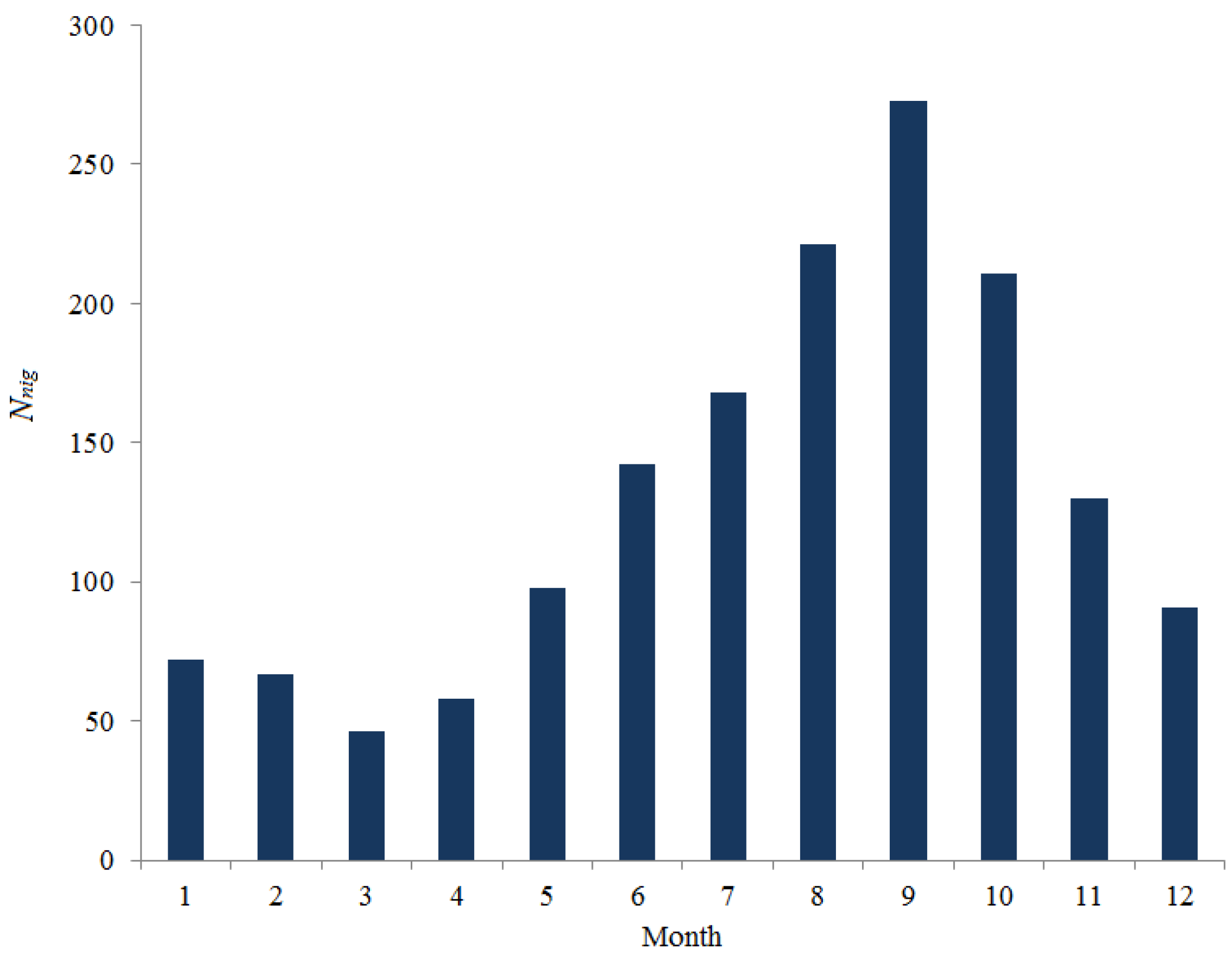
The approach based on the application of a deep neural network has a certain merit, as it allows one to search for internal relations between seeing variations and the evolution of some background states of atmospheric layers at different heights. We use the medians of seeing estimated from measurements of differential displacements of stellar images at the site of the Maidanak observatory as predicted values. We should note that routine measurements of star image motion are made at the Maidanak observatory using the Differential Image Motion Monitor (DIMM) [26,27]. The database of measured seeing is available for two periods: 1996–2003 and 2018–2022. In Figure 1, we present the total amount of DIMM data for each month during the acquisition period. The 13-year dataset used covers a variety of atmospheric situations and is statistically confident. Analysis of Figure 1 shows that the fewest number of nights used for machine learning occurs in March. The best conditions correspond to August–October, when the observatory has a good amount of clear time.

The observed difference in the number of nights for different months is related to the atmospheric conditions limiting the observations (strong surface winds and high-level cloud cover).

Also, we used data from the European Center for Medium-Range Weather Forecast Reanalysis (Era-5) [28] as inputs for training the neural networks. Meteorological characteristics at different pressure levels were selected from the Era-5 reanalysis database for two periods: 1996–2003 and 2018–2022. Night-to-night averaging of the reanalysis data corresponds to the averaging of measured seeing.

3.1. Era-5 Reanalysis Data

Reanalysis Era-5 is a fifth-generation database. The data in the Era-5 reanalysis are presented with high spatial and temporal resolution. The spatial resolution is 0.25${}^{\circ }$, and the time resolution is 1 h. Data are available for pressure levels ranging from 1000 hPa to 1 hPa. In simulations, in addition to hourly data on pressure levels, we also used hourly data on single levels (air temperature at a height of 2 m above the surface and horizontal components of wind speed at a height of 10 m above the surface).

We have verified the Era-5 reanalysis data for the region where the Maidanak Astronomical Observatory is located. Verification was performed by comparing semi-empirical vertical profiles of the Era-5 reanalysis with radiosounding data at the Dzhambul station. Dzhambul is one of the closest sounding stations to the Maidanak Astronomical Observatory.

In order to numerically estimate the deviations of the reanalysis data from the measurement data, we calculated the mean absolute errors and the standard deviations of air temperature and wind speed. The mean absolute errors and the standard deviations were estimated using the formulas [29]:

$$\Delta T=\frac{1}{N}\sum _{i=1}^N\mid T_i\left(z\right)(Era-5)-T_i\left(z\right)\left(rad\right)\mid ,$$

(9)

$$\Delta V=\frac{1}{N}\sum _{i=1}^N\mid V_i\left(z\right)(Era-5)-V_i\left(z\right)\left(rad\right)\mid ,$$

(10)

$${\sigma }_T={\left(\frac{1}{N}\sum _{i=1}^N{\left(T_i\left(z\right)(Era-5)-T_i\left(z\right)\left(rad\right)\right)}^2\right)}^{0.5},$$

(11)

$${\sigma }_V={\left(\frac{1}{N}\sum _{i=1}^N{\left(V_i\left(z\right)(Era-5)-V_i\left(z\right)\left(rad\right)\right)}^2\right)}^{0.5},$$

(12)

where z is the height and $\Delta T$ and $\Delta V$ are the mean absolute errors of air temperature and wind speed, respectively. Brackets $(Era-5)$ and $\left(rad\right)$ indicate the type of data (Era-5 reanalysis and radiosondes). ${\sigma }_T$ and ${\sigma }_V$ are the root mean square deviations of air temperature and wind speed, respectively. N includes all observations for January 2023 and July 2023.

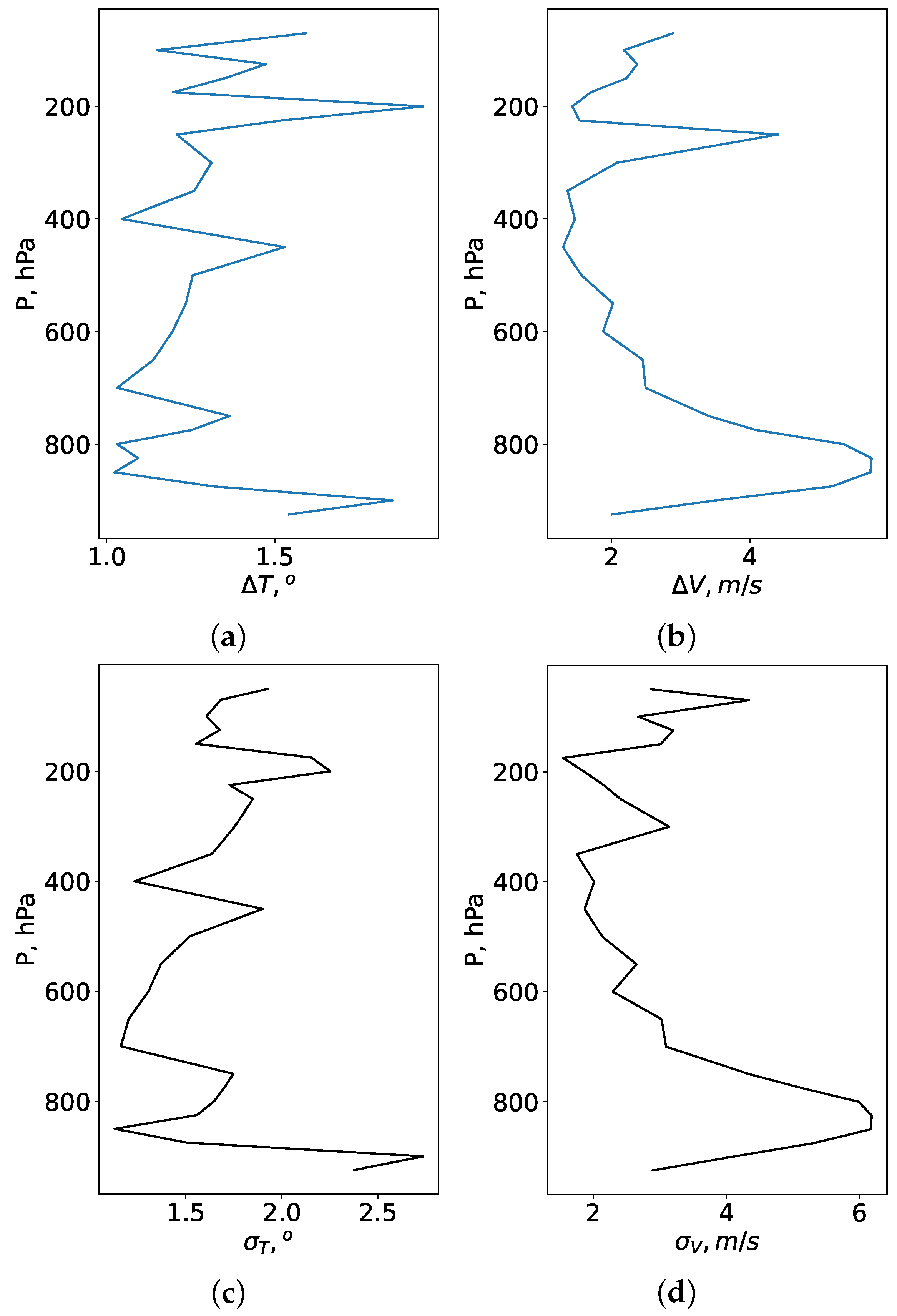
Figure 2 and Figure 3 show the vertical profiles of $\Delta T$, $\Delta V$, ${\sigma }_T$, and ${\sigma }_V$. The profiles are averaged over June–August and December–February. Analysis of these figures shows that, in winter, $\Delta T$, $\Delta V$, ${\sigma }_T$, and ${\sigma }_V$ are 1.3${}^{\circ }$, 2.8 m/s, 1.7${}^{\circ }$, and 3.3 m/s, respectively. In winter, the high deviations of measured air temperature from the reanalysis-derived values are observed mainly in the lower layer of the atmosphere (up to 850 hPa). We attribute these deviations to the inaccuracy of modeling surface thermal inversions and meso-jets in the reanalysis. Above the height corresponding to the 850 hPa level, the deviations decrease significantly ($\Delta T$∼1.2${}^{\circ }$, ${\sigma }_T$ = 1.5${}^{\circ }$). In vertical profiles of wind speed, the character of height change in the wind is more ordered. In particular, significant peaks are observed in the entire thickness of the atmosphere. The standard deviation of wind speed in the atmospheric layer up to the 850 hPa level (in the lower atmospheric layers) is higher than 6.0 m/s. In the layer above the 850 hPa pressure level, $\Delta V$ and ${\sigma }_V$ decrease to 1.8 m/s and 2.2 m/s, respectively.

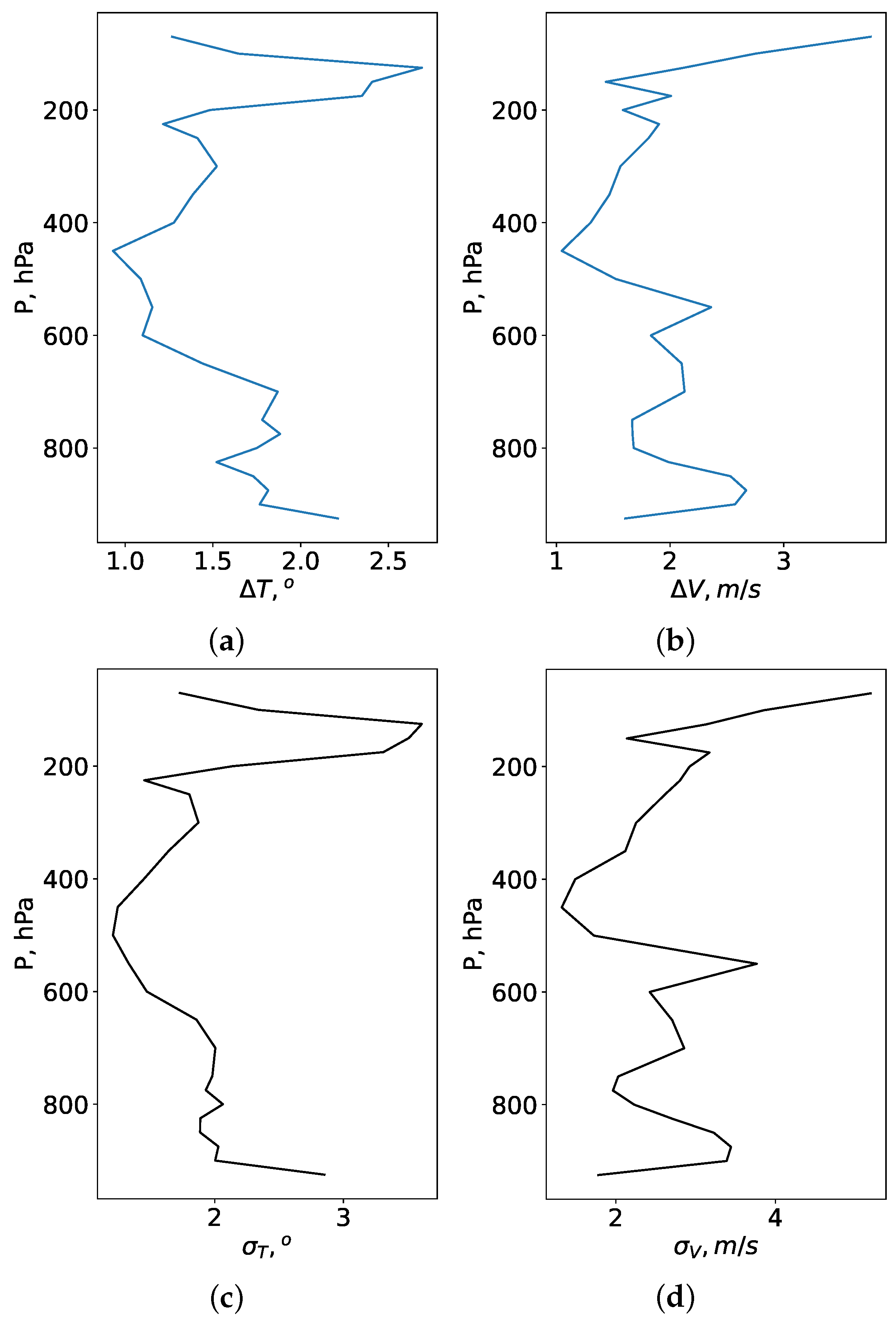
In summer, temperature deviations between radiosonde and Era-5 data decrease. Analysis of Figure 3 shows that these deviations are due to the fact that the reanalysis often does not reproduce correctly the large-scale jet stream. Also, in summer, the Era-5 reanalysis overestimates the surface values of air temperature. $\Delta T$ and ${\sigma }_T$ in the entire atmosphere are 1.7${}^{\circ }$ and 2.3${}^{\circ }$, respectively. ${\sigma }_T$ values are 2.8${}^{\circ }$ and 3.6${}^{\circ }$ within the lower atmospheric layers and at the height of the large-scale jet stream, respectively.

Considering wind speed, the deviations between the measured and modeled parameters are pronounced. $\Delta V$ and ${\sigma }_V$ are 2.2 m/s and 2.7 m/s, respectively. In the lower layers of the atmosphere, the mean absolute error and the root mean square deviation are 2.9 m/s and 3.6 m/s. High deviations in the wind speed correspond to the atmospheric levels under a large-scale jet stream (200 hPa). Within the upper atmospheric layers, ${\sigma }_V$ can reach 4.0 m/s.

Thus, in this section we examine how well the reanalysis data, corresponding to a certain computational cell, describe the real vertical profiles of wind speed and air temperature. In general, there are some atmospheric situations when reanalysis reproduces profiles with a large error. Reanalysis does not reproduce thin thermal inversions or mesojet streams in the lower atmospheric layers and overestimates or underestimates the speed of air flow in a large-scale jet stream. In order to increase the efficiency of training neural networks, below also we consider model weather data with the best reproducibility of vertical changes. In training, we used meteorological characteristics at all available pressure levels from 700 hPa to 3 hPa. The selection of the lower pressure surface corresponding to 700 hPa is determined by the elevation of the observatory (2650 m, surface pressure $P_{surf}$ is equal to 733 hPa) and surrounding areas above sea level.

3.2. Seeing Values Derived from Image Motion Measurements

The predicted value is the median of seeing averaged over the night. Seeing is the parameter calculated from image motion measurements. The theory for calculating seeing based on image motion measurements is described in the paper [7]. Using the Kolmogorov model, seeing may be estimated based on the following relation:

$${\sigma }_{\alpha }^2=K{\lambda }^2{r}_0^{-5/3}{D}^{-1/3},$$

(13)

where $\lambda$ is the light wavelength and D is the telescope diameter. The variance in the differential image motion is denoted ${\sigma }_{\alpha }^2$. This quantity is related to the Fried parameter $r_0$ by the formula:

$$seeing=0.98\frac{\lambda }{r_0},$$

(14)

Coefficient K in Formula (13) depends on the ratio of the distance between the centers of apertures $S_d$ and the aperture diameter $d_s$, the direction of image motion, and the type of tilt. The coefficients for longitudinal and transverse motions are determined by the gravity center of the images:

$$K_l=0.34\left(1-0.57{\left(\frac{S_d}{d_s}\right)}^{-1/3}-0.04{\left(\frac{S_d}{d_s}\right)}^{-7/3}\right),$$

(15)

$$K_t=0.34\left(1-0.855{\left(\frac{S_d}{d_s}\right)}^{-1/3}+0.03{\left(\frac{S_d}{d_s}\right)}^{-7/3}\right).$$

(16)

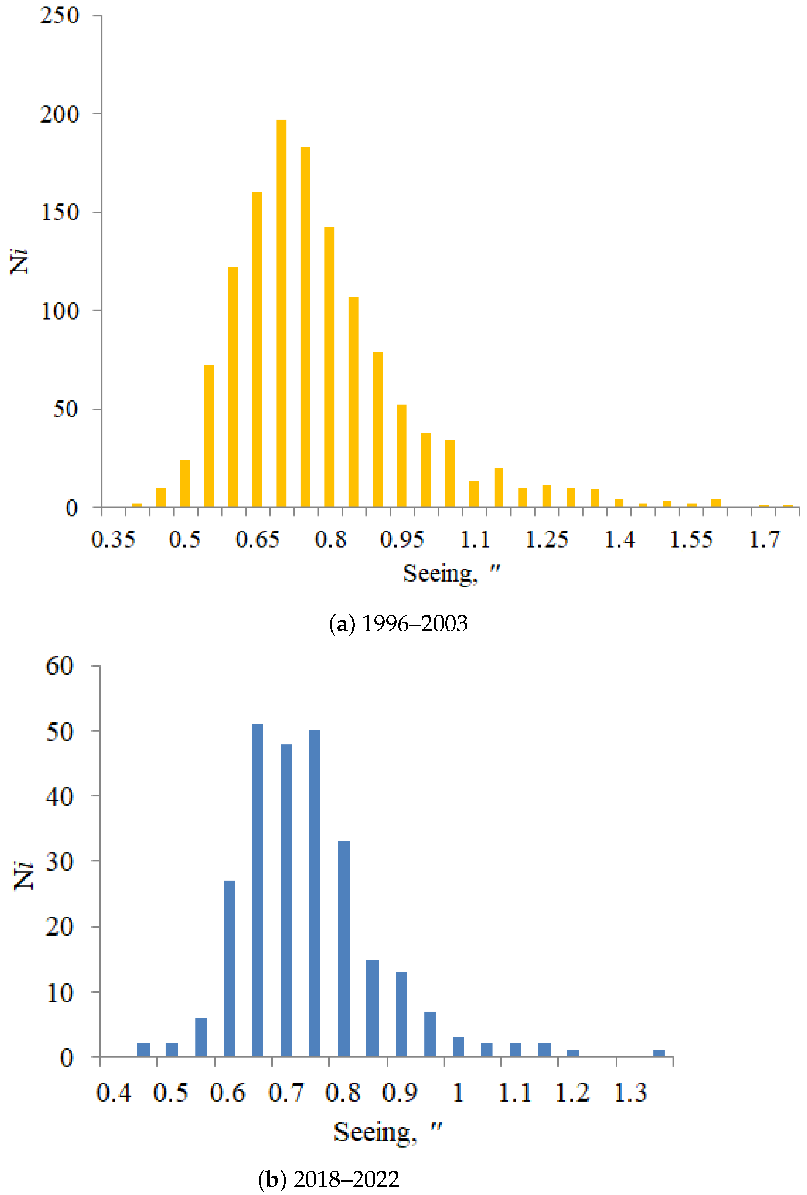
Using all data of measurements we computed the seeing values, shown as the histograms in Figure 4a,b. Analysis of Figure 4a,b shows that the range of changes in the integral intensity of optical turbulence at the Maidanak Astronomical Observatory site is narrow. The bulk of the values fall within the range from 0.6 to 0.9${}^{″}$. Despite the narrow range of seeing changes, we can note that the neural networks have been trained for a wide range of atmospheric situations.

4. Neural Network Configuration for Estimation of Seeing

An artificial neural network is a complex function that connects inputs and outputs in a certain way. The construction of a neural network is an attempt to find internal connections and patterns between inputs, their neurons, and outputs in the study of phenomena and processes. The aims of this study is to show how capable an artificial neural network is of estimating seeing variations for the Maidanak Astronomical Observatory, which is located in the most favorable atmospheric conditions.

A flowchart for the creation of neural networks is shown in Figure 5. According to this flowchart, the initial time series are divided into training, checking, and validation datasets. The main stage is training the neural network and generation of partial models. In particular, learning is based on data pairs of observed input and output variables. Using different inputs (meteorological characteristics) we optimized the final structure of the neural network.

An important step in seeing simulation with neural networks is the selection of input variables. The inputs are selected based on the physics of turbulence formation described in Section 2. According to the theory, the formation of turbulent fluctuations in the air temperature and, consequently, the air refractive index is largely determined by the advection of air masses, the rate of dissipation of fluctuations, as well as vertical turbulent flows, which depend on vertical gradients of meteorological characteristics. In addition, the turbulence structure is closely related to large-scale atmospheric disturbances, including meso-scale jet streams and large atmospheric turbulent vortices. In particular, the inputs are wind speed components, air temperature and humidity, vorticity of air flows, and the values of surface turbulent stresses. The final configuration of the neural network is formed by excluding neurons whose weights are minimal. As we will see below, the neural networks obtained that best reproduce the seeing variations do not contain neurons functionally related to atmospheric vortices.

To create configurations of neural networks connecting inputs and outputs, we chose the group method of data handling (GMDH) [30,31,32]. The GMDH method is based on some model of the relationship between the free variables x and the dependent parameter y (seeing) [33]. To identify relationships between the turbulent parameter seeing averaged during the night and vertical profiles of mean meteorological characteristics, we used the Kolmogorov–Gabor polynomials, which are the sum of linear covariance, linear, quadratic, and cubic terms [30]:

$$y=W_0+\sum _{i=1}^m{W}_i{x}_i+\sum _{i=1}^m\sum _{j=1}^m{W}_{ij}{x}_i{x}_j+\sum _{i=1}^m\sum _{j=1}^m\sum _{k=1}^m{W}_{ijk}{x}_i{x}_j{x}_k+...$$

(17)

In Formula (17), the index m denotes the set of free variables and $W_i$,$W_{ij}$,$W_{ijk}$ are the weights. Seeing is considered as a function of a set of free variables [30]:

$$seeing=f(x_1,x_2,x_1{x}_2,x_1^2....)=F(z_1,z_2,z_3....).$$

(18)

The modeled $seein{g}_{\ast }$ can be expressed in the following shape [30]:

$$seein{g}_{\ast }=W_0+\sum _{i=1}^{F_0}{W}_i{z}_i=W_0+Wz,$$

(19)

where $Wz$ is a scalar product of two vectors. The correct estimation of the outputs is mainly determined by the trained parameters—the weights W. The goal of training is to find the weights at which the created neural network produces minimal errors.

The result of applying the GMDH method is a certain set of neural network models containing internal connections between input meteorological parameters, their derivatives, and the output. The best solution must correspond to the minimum of the loss function, the values of which depend on all weights. The loss function can be written as [30]:

$$R_{ext}\left(validate\right)={\left(\frac{1}{M}\sum _{i\in validate}^M{(seein{g}_i-seein{g}_{i\ast }\left(training\right))}^2\right)}^{0.5},$$

(20)

The loss function $R_{ext}\left(check\right)$ is estimated using validation data (new data).

Finding the minimum of the loss function is a rather difficult task due to the multidimensionality of the function, determined by the number of input variables. To find the minimum of the loss function from the training dataset, a gradient descent algorithm is used based on calculating the error gradient vector (partial derivatives of the loss function over all weights). In simulations, the initial weights are initialized randomly and are small. The weights are updated or adjusted using error backpropagation method (from the last neural layer to the input layer). In this method, the calculation of derivatives of complex functions makes it possible to determine the weight increments in order to reduce the loss function. In this case, for each output neuron with the number of the layer $N_{neur+1}$, the errors and weight increments are calculated and propagated to the neurons in the previous layer $N_{neur}$. The optimal neural network should correspond to the minimum of this loss function $R_{ext}\left(validate\right)$.

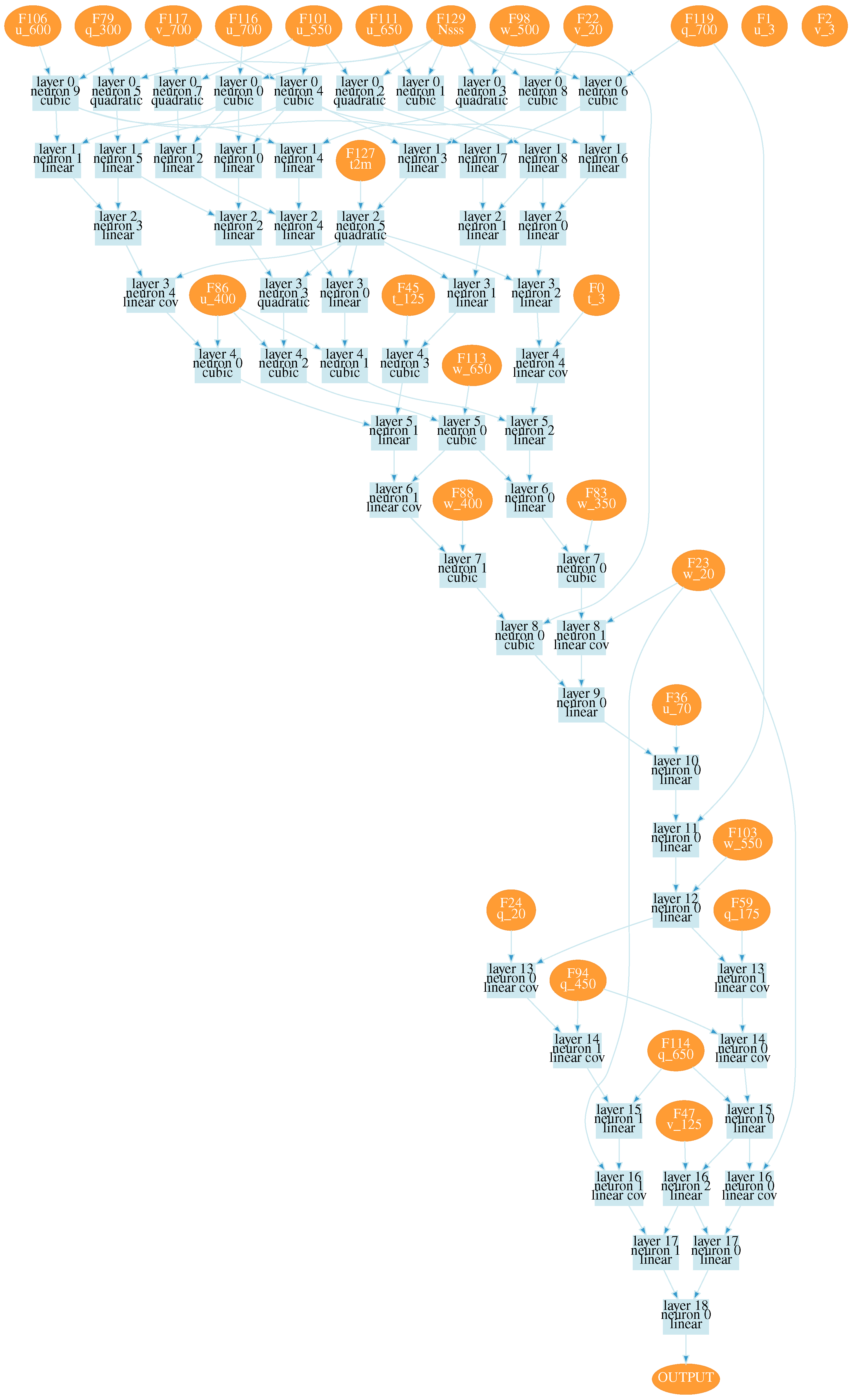
After training, we received a wide set of neural network configurations for estimating seeing. Estimating values of the loss function, two neural network configurations were chosen, shown in Figure A1 and Figure A2. These configurations are obtained using all training data. Numbers on the right side of variables in the figures correspond to pressure levels. Designations used in neural networks are given in

Table 1. Designations used in neural networks.

Label	Parameter
nsss	northward turbulent surface stress
u	u-component of wind
v	v-component of wind
w	w-component of wind
q	specific humidity
t	air temperature
$t2m$	air temperature at height of 2 m

. The input atmospheric characteristics, the number of layers, and the neural network structure are automatically determined in the used learning algorithm.

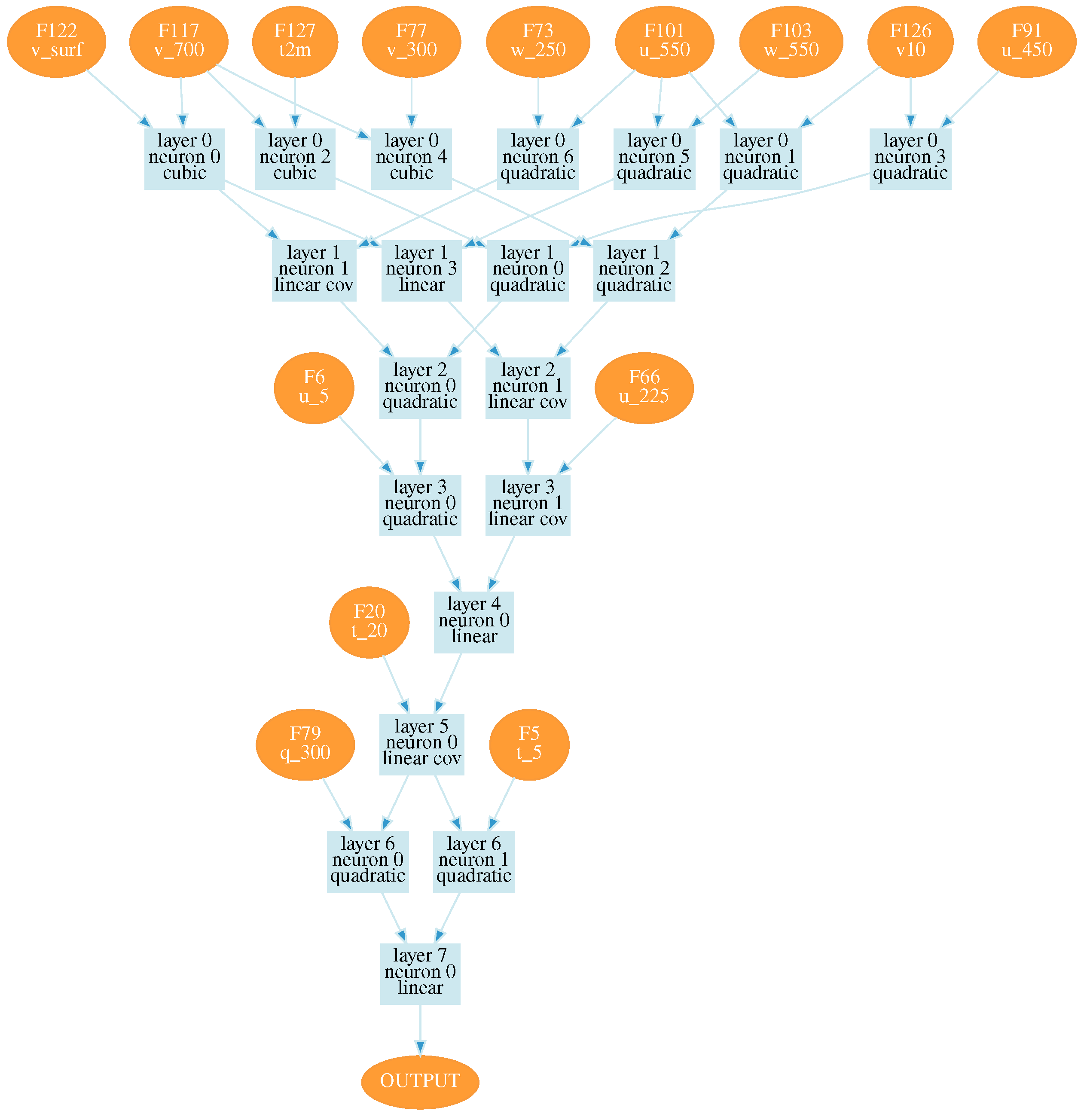
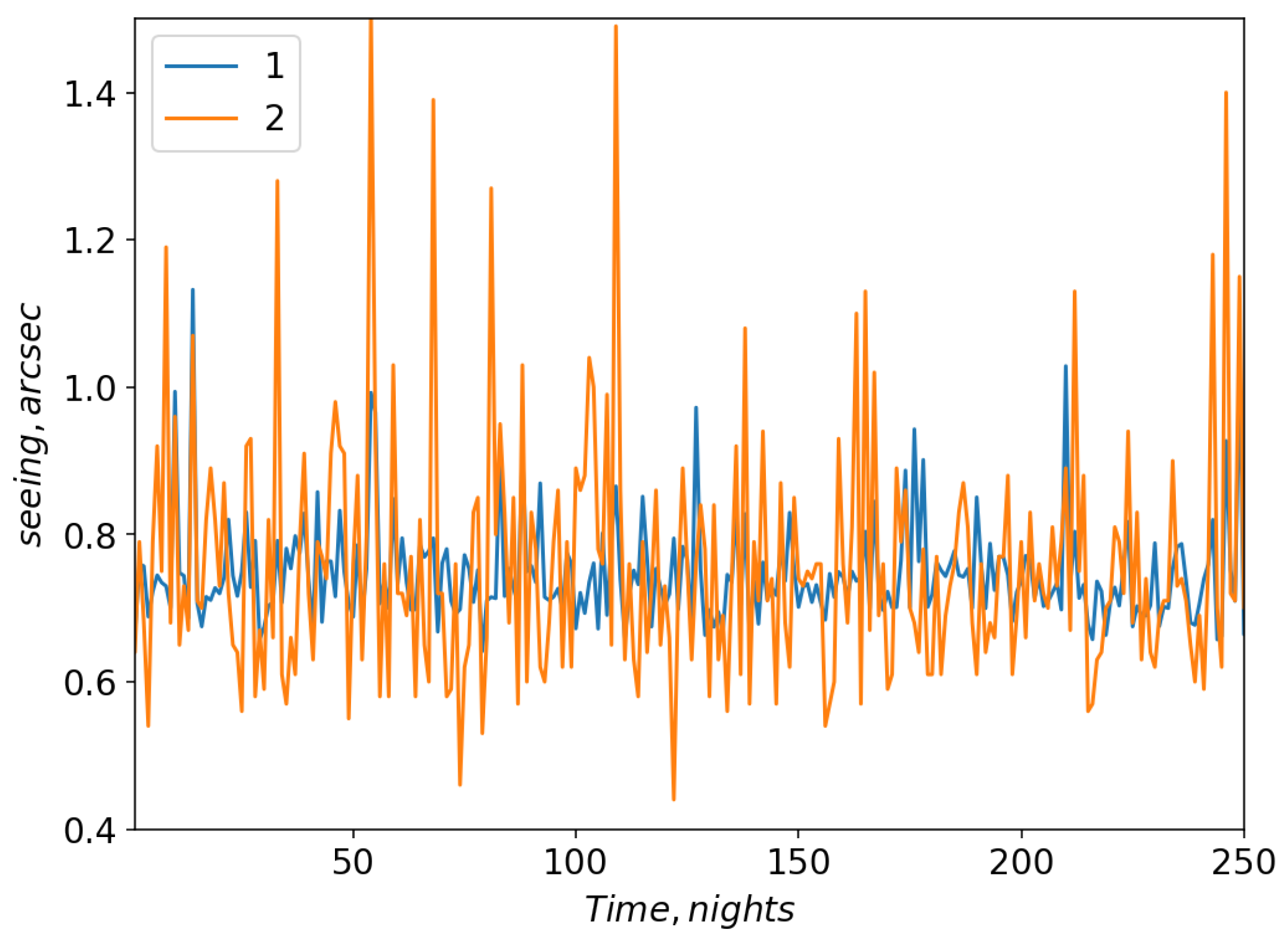
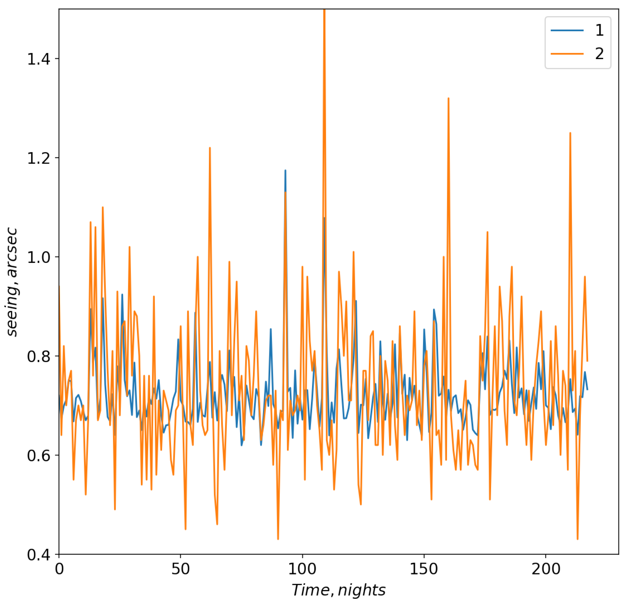
These configurations correspond to the minima of the loss function; the values of the functions are close to 0.04${}^{″}$. At the same time, the configuration shown in Figure A2 shows a better reproducibility of seeing variations. Figure 6 and Figure 7 show changes in the model and measured seeing values for neural network configurations 1 and 2, respectively.

For these configurations, the linear Pearson correlation coefficient between the model and measured seeing values reached 0.67 and 0.7, respectively (the training datasets). For the validation dataset, the linear Pearson correlation coefficient for configuration 1 was 0.49; for configuration 2 the correlation coefficient increased to 0.52. Thus, using all data, the efficiency of training a neural network that predicts variations in seeing is not very high.

The training process identified important inputs. An analysis of the obtained neural network configurations shows that the main parameters that determine the target values of total seeing are northward surface turbulent stresses and wind speed components on the model levels closest to the summit, that is, 650 and 700 hPa. We also should emphasize that there is a degradation of the statistical measures associated with excluding surface turbulent stresses from the training process. Neural network configurations obtained with excluded surface turbulent stresses demonstrate low correlation coefficients ∼0.3. Also, meaningful characteristics in determining atmospheric seeing are wind speed components at the 250 hPa level and air temperature at 2 m with minor contributions. Atmospheric situations with high air humidity show a negligible influence.

Development of neural network configurations using the GMDH method for the Maidanak Astronomical Observatory was complicated by certain conditions. At the Maidanak Astronomical Observatory, atmospheric conditions with low optical turbulence energy along the line of sight, and, more importantly, with small amplitudes of change in the magnitude of seeing from night to night are often observed. In order to optimize the learning process and find a network with better reproducibility of seeing variations, we filtered the initial data. The conditions of filtering are:

(i)

We chose only atmospheric situations with the cloud fraction in the calculated cell less than 0.3.

(ii)

We excluded nights when the vertical profiles of wind speed and air temperature obtained from the reanalysis data significantly deviated from the reference vertical profiles (from data measured at the Dzhambul radiosounding station).

(iii)

We retained only nights with more than 50 measurements of optical turbulence per night. Nights with a low quantity of measurement data correspond to unfavorable atmospheric conditions (strong surface winds and upper cloudiness).

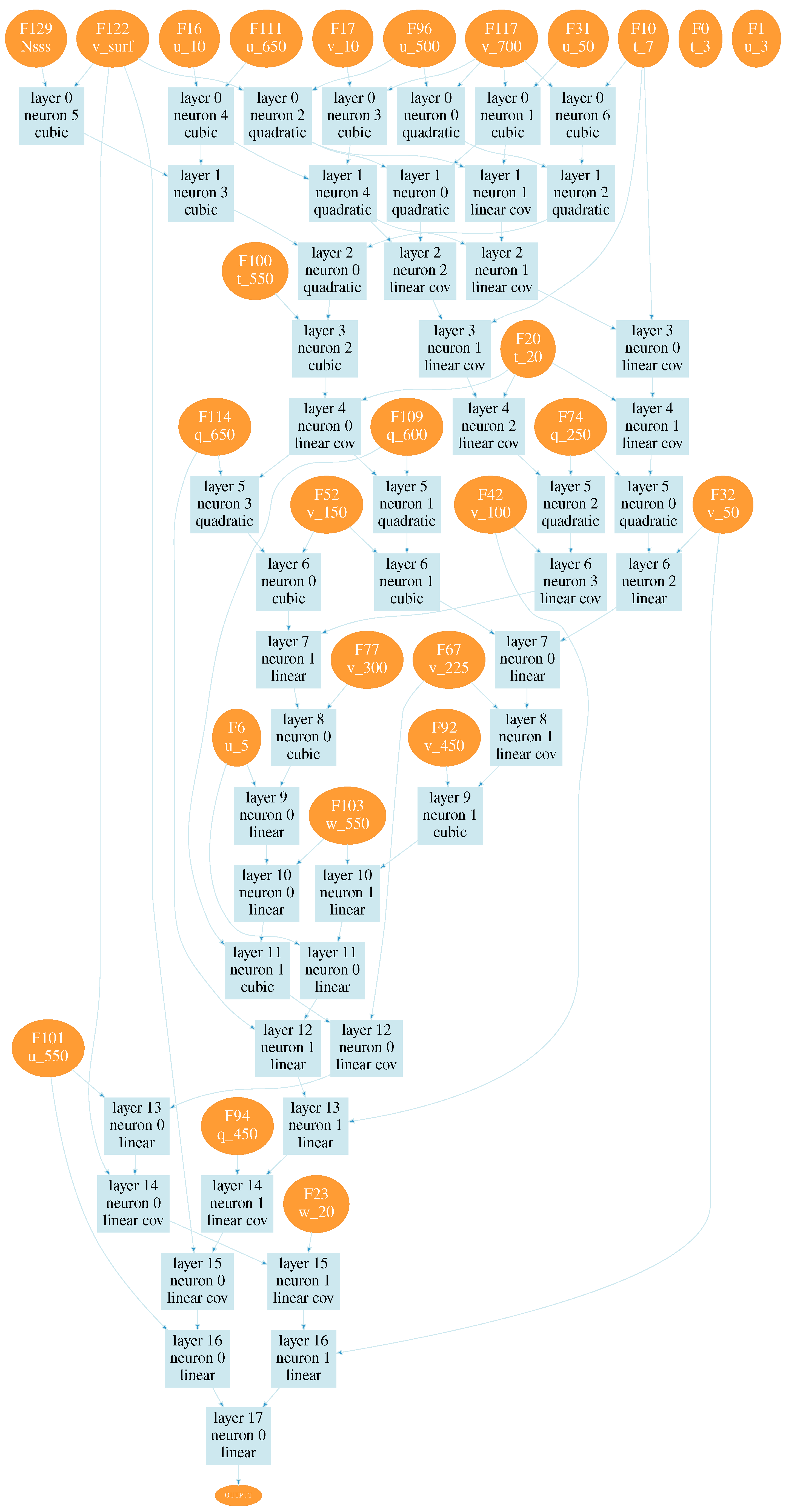
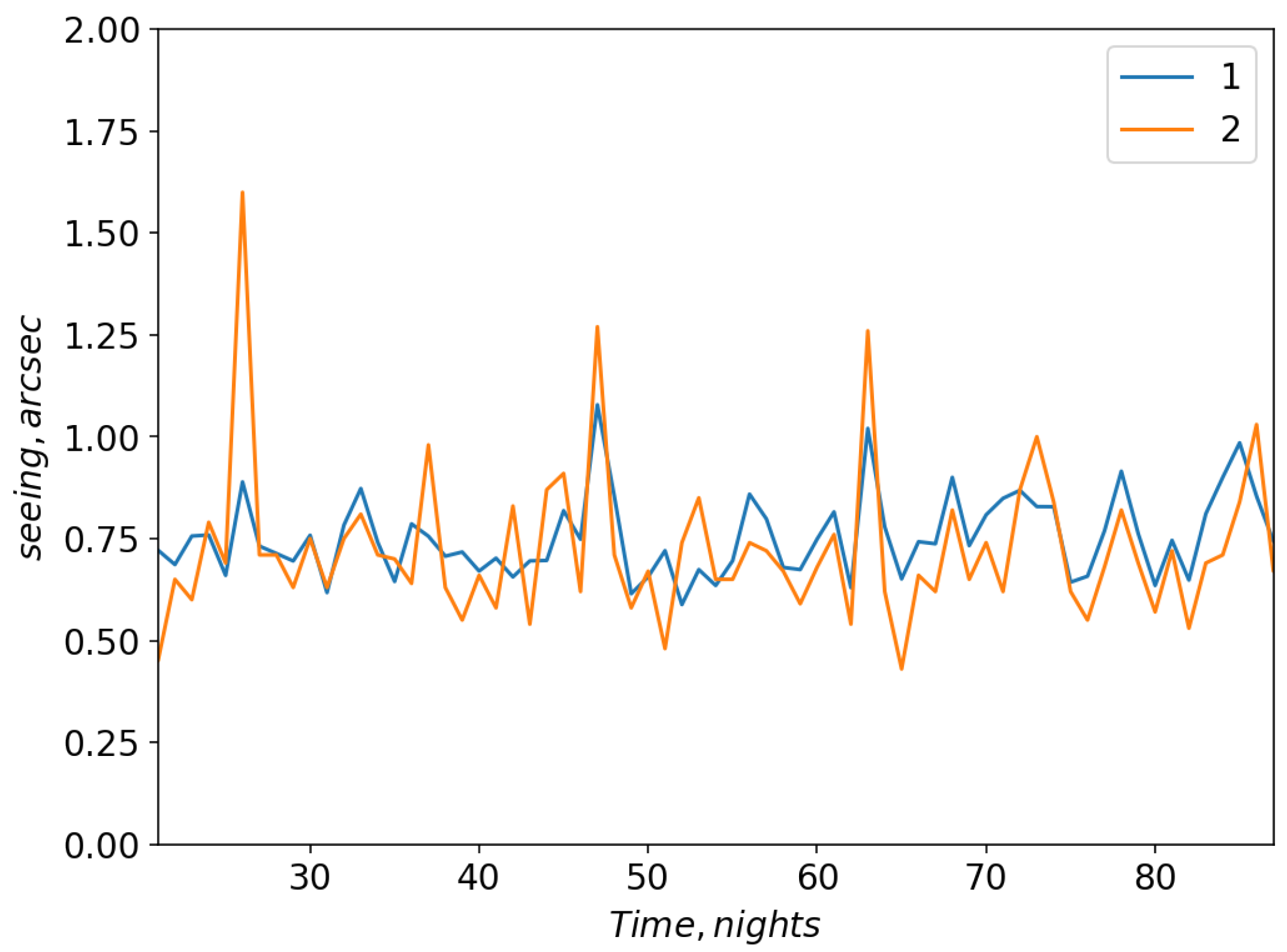
Since the reanalysis demonstrates the highest deviations precisely for the lower layers of the atmosphere, we excluded most of the atmospheric processes when seeing was determined primarily by the influence of low-level turbulence. In particular, the 20 percent of nights corresponding to the highest deviations in air temperature and wind speed in the lower atmospheric layers were excluded. The corresponding configuration of the optimal neural network is shown in Figure A3.

For this configuration, Figure 8 shows changes in the model and measured seeing. The correlation coefficient between the measured and model variations is higher than for configurations 1 and 2 and equal to 0.68. Neurons of this network contain such atmospheric variables as u at 225 hPa and v in the lower atmospheric layers (700 hPa). For the neural network shown in Figure A3, large-scale atmospheric advection begins to play the greatest role (u at 550 hPa). Using this neural network, we also estimated the median value of seeing at the Maidanak observatory site during the period from January to October 2023. This median value of seeing is 0.73${}^{{}^{″}}$.

Analysis of the neural networks obtained shows that individual bright connections between neurons are substituted for most configurations with nearly equal-weight coefficients. Unlike the Sayan Solar Observatory, the deep neural networks obtained for the Maidanak Astronomical Observatory do not contain pronounced connections between the seeing parameter and atmospheric vorticities [34]. Moreover, the use of atmospheric vorticities in the simulation even slightly reduces the Pearson correlation coefficient between the model and measured seeing values. For neural networks containing atmospheric vorticities, the Pearson correlation coefficient is reduced less than 0.45. In our opinion, this is due to the fact that the effect of large-scale atmospheric vorticity on optical turbulence at the Maidanak Astronomical Observatory site is minimal and it is noticeable only for individual time periods when the seeing value increases.

5. Conclusions

The following is a summary of the conclusions.

This paper focuses on developing physically informed deep neural networks as well as machine learning methods to predict seeing. We proposed ensemble models of multi-layer neural networks for the estimation of seeing at the Maidanak observatory. As far as we know, this is the first attempt to simulate seeing variations with neural networks at the Maidanak observatory. The neural networks are based on a physical model of the relationship between the characteristics of small-scale atmospheric turbulence and large-scale meteorological characteristics relevant to the Maidanak Astronomical Observatory.

For the first time, configurations of a deep neural network have been obtained for estimating seeing. The neurons of these networks are linear, quadratic, cubic, and covariance functions of large-scale meteorological characteristics at different heights in the boundary layer and free atmosphere. We have shown that the use of a different set of inputs makes it possible to estimate the influence of large-scale atmospheric characteristics on variations in the turbulent parameter seeing. In particular, the present paper shows that:

(i)

The seeing parameter weakly depends on meso-scale and large-scale atmospheric vorticity, but is significantly sensitive to the characteristics of the surface layer of the atmosphere. In particular, for neural networks containing atmospheric vorticities, the Pearson correlation coefficient is low, ∼0.45.

(ii)

The air temperature and wind speed at the pressure levels closest to the observatory, as well as the northward turbulent surface stress, have a significant impact on seeing. Applying the northward turbulent surface stress parameter in the training process makes it possible to improve significantly the retrieving seeing variations (the Pearson correlation coefficient increases from 0.45 to ∼0.70). The estimated median value of seeing with neural networks at the Maidanak observatory site during the period from January to October 2023 is 0.73${}^{″}$.

(iii)

The influence of the upper atmospheric layers (below the 200 hPa surface) becomes noticeable for selected atmospheric situations when, as we assume, the reanalysis best reproduces large-scale meteorological fields.

Verification of the hourly averaged vertical profiles of wind speed and air temperature derived from the Era-5 reanalysis database was performed. We compare semi-empirical vertical profiles of the Era-5 reanalysis with radiosounding data of the atmosphere at the Dzhambul station, which is located within the region of the Maidanak Astronomical Observatory. The largest deviations correspond to the lower layers of the atmosphere and the pressure levels of a large-scale jet stream formation. In winter, $\Delta T$, $\Delta V$, ${\sigma }_T$, and ${\sigma }_V$ are 1.3${}^{\circ }$, 2.8 m/s, 1.7${}^{\circ }$, and 3.3 m/s, respectively. In summer, these statistics have similar values: 1.7${}^{\circ }$, 2.2 m/s, 2.3${}^{\circ }$, and 2.7 m/s, respectively.