Modeling the Normalized Urban Heat Island for the City of Karlsruhe by Linking Urban Morphology and Green Infrastructure

Abstract

Citizens in urban areas are affected by the urban heat island (UHI) effect, resulting in increased thermal heat compared to rural areas. This threat is exacerbated by global climate change. Therefore, it is necessary to assess human thermal comfort and risk for decision making. This is important for planners (climate resilience), the health sector (information for vulnerable people), tourism, urban designers (aesthetics), and building architects. Urban structures modify local meteorological parameters and thus human thermal comfort at the microscale. Knowledge of the pattern of a city’s UHI is typically limited. Based on previous research, generalized additive models (GAMs) were built to predict the spatial pattern of the UHI in the city of Karlsruhe. The models were trained with administrative, remotely sensed, and land use and land cover geodata, and validated with measurements in Freiburg. This identified the hot and cold spots and the need for further urban planning in the city. The model had some limitations regarding water bodies and anthropogenic heat production, but it was well suited for applications in mid-latitude cities which are not topographically characterized. The model can potentially be used for other cities (e.g., in heat health action plans) as the training data are freely available.

1. Introduction

By 2050, 6.7 billion people (68% of the world’s population) will live in cities [1]. Urban environments, determined by climatic effects from the prevailing mesoscale down to the microscale, affect the urban quality of life. This mainly refers to the urban bioclimate, air quality, traffic, and noise pollution in street canyons at the microscale [2,3,4]. Therefore, the bioclimate, and hence human thermal comfort, is severely threatened by the urban heat island (UHI) effect, global climate change, increasing heat waves and heat events, further sealing, and the densification of urban areas [5,6]. In order to make appropriate decisions, it is essential to obtain detailed information on the spatial pattern of the UHI to identify areas where action is needed. Detailed information should be used for climate-adapted resilient urban planning to cover nature-based as well as artificial solutions for heat mitigation (e.g., unsealing, green facades, green roofs, white roofs, PV-equipped roofs, new unsealed surfaces, cool shelters, cool fountains, the optimization of street configurations and parks, etc.) [7,8,9,10,11].

Many studies have focused on the quantification of the UHI effect by remote sensing analyses, particularly on the evaluation of the land surface temperature (LST). Unfortunately, these methods themselves are insufficient for human-biometeorological purposes. The spatial and temporal resolution of satellite imagery is usually insufficient for the microscale analyses of urban areas (e.g., 30 $\mathrm{m}$ resolution of Landsat 7 and 8 and 20 $\mathrm{m}$ resolution of Sentinel-2 for the assessment of infrared) [12,13]. The temporal resolution is restricted to the overpass time of the spaceborne platform and the cloud cover of the surface; i.e., a full assessment of the diurnal cycle of the surface UHI (S-UHI) is not possible [13]. The energy conversions on the vertical surfaces or facades are angular in function of the surface’s position with regard to the sun and towards the sensor, and thus it cannot be fully captured by remote sensing instruments due to effective anisotropy [14]. For example, off-nadir observations were up to $3.5$ $\mathrm{K}$ cooler on average than nadir LST, as shown in a case study by [15]. In addition, the complexity of the human thermal bioclimate cannot be reduced to the assessment of the land surface temperature, but requires the assessment of all atmospheric conditions (air temperature, relative humidity or vapor pressure, wind speed, and long- and shortwave radiation in terms of mean radiant temperature) and human thermoregulation (based on the parameters of the human body) in urban environments [16]. At the same time, it is not possible to directly measure air temperature or humidity by space-borne remote sensing platforms, but it is possible to measure LST resulting in S-UHI in urban environments [17]. To overcome this limitation, attempts were made to determine the statistical correlation between LST and near-surface air temperature ($T_a$) [18]. Correlations were found on a regional or global scale (1– 2 $\mathrm{k}$$\mathrm{m}$), especially under cloudy conditions, which are not present during extreme heat events. In a complex urban environment, at the microscale, this is even more challenging, as horizontal surfaces are mostly observed by satellites, but the global radiation is trapped in vertical three-dimensional street canyons in particular. At the same time, surface properties (albedo and emissivity) vary greatly in a city and lead to a modified energy balance and surface temperatures. In order to determine the air temperature in the urban canopy layer (UCL), further analyses were carried out based on LST by Moderate Resolution Imaging Spectroradiometer (MODIS) installed on the Terra and Aqua satellites [19]. These approaches were supplemented by additional information regarding the vegetation, water, and course of the sun (enhanced vegetation index, normalized difference water index, solar zenith angle, and distance to coast) to determine the mean $T_a$ in Shanghai during the period 2000–2013 with an root mean square error ($RMSE$) of 1.6– $2.6$ ${}^{\circ }\mathrm{C}$ [20].

In situ observations, spatial surveys, traverses, long-term urban networks, and citizen weather stations have been used by others, as opposed to remotely sensed measurements, to determine the characteristics of the UHI or rather the urban heat archipelago based on mobile air temperature measurements. Based on these measurements, statistical machine learning (ML) approaches have been used in the past to determine the UHI with high spatial resolution over the entire study area [21,22,23,24,25]. In order to spatially analyze the urban microclimate, at the very least, data on the land use, building morphology, and vegetation are mandatory [12]. The combination of satellite data (LST from Sentinel-2 or Landsat 8) and in situ measurements by a statistical model is not new either [26,27,28]. In those studies, the air temperature observations from a citizen science-driven measurement campaign were used to predict the UHI extremes using ML (random forest (RF)). The used algorithm was trained with descriptors for land use and land cover (LULC), derived from the survey imagery. Other authors also used RF and extreme gradient boosting to predict the UHI pattern and trained the models based on multi-platform observations [29,30]. Crowd-sourced data (e.g., Netatmo) were also used in other studies to obtain a comprehensive, urban-wide dataset with further ML models (RF, gradient boosting, and model averaged neural network) [31,32,33]. Gradient boosting was used to predict the maximum air temperature at a spatial resolution of 1 $\mathrm{k}$$\mathrm{m}$${}^2$ using urban wide LST, normalized difference vegetation index (NDVI), digital elevation model (DEM), Julian day, and solar zenith angle [34]. In addition to the aforementioned predictors, others used urban heatwave thermal index (UHTI) maps based on LST, vegetation fraction cover (VFC), and sky view factor (SVF) to predict the spatially resolved physiologically equivalent temperature (PET) at a 10 $\mathrm{m}$ resolution [35,36]. They used linear regression to link LST, VFC, or SVF to air temperature. The calculation of PET was based on the combination of ENVI-met simulations and Bio-met tool. However, it remains questionable whether LST, VFC, and NDVI can be used simultaneously as predictors, as they are linearly dependent on each other, and whether the respective relationship between LST, VFC, SVF, and $T_a$ can be represented by single linear regressions without interactions.

In this study, the intention was to spatially quantify the pattern of the UHI for the whole city and throughout the day. The quantification was based on remotely sensed data, in situ observations, and the administrative data of the municipality of Karlsruhe to describe the microscale effects of the urban morphological surroundings on the normalized air temperature in 2 $\mathrm{m}$ as well as on the bioclimate (Section 2). Urban morphology represents the size, shape, and physical structure of a city [37] and can be studied from different perspectives with different foci. The consideration of the urban morphology by means of land use classification (e.g., Urban Atlas 2018 (UA 2018), local climate zones (LCZ), CORINE land cover (CLC), and urban climate zones (UCZ)) provides a summarizing overview of the distribution of urban, industrial, and green areas in a city [38,39,40,41]. Each type of land use is characterized by a different degree of building development, sealing, and greening, resulting in different (thermal) environments. Each environment, in turn, is characterized by different resulting meteorological conditions depending on the energy balance of the immediate surroundings, i.e., the thermal properties (heat storage capacity), radiative properties (albedo, emissivity), and thus, sensible, latent, and radiative heat fluxes [42,43]. In order to evaluate the thermal effects of individual urban trees and buildings at the microscale in an open system (such as the urban environment), it is not sufficient to only consider land use, as the diversity (of buildings and trees) cannot be represented by these classes. In particular, vertical surfaces cannot be resolved by these classes. The morphology of the urban gray infrastructure can be defined by the arrangement of buildings, surface materials, and the degree of sealing. The real estate cadasters of the city of Karlsruhe contained information on spatially resolved 3D buildings in CityGML format. These data provided additional detailed information on the density and heights of the buildings, which were missing in the land use classes. The morphology of the urban green infrastructure describes the allometry, species composition, and spatial arrangement of the vegetation in the city. The cooling potential of green infrastructure depends on the allometric parameters (crown dimension, tree height, and leaf area) as well as the density and composition of different tree species in a group of trees [44,45]. The urban blue infrastructure includes all water bodies (lakes and rivers) in the city. It is generally assumed that, depending on their depth, these bodies of water have a cooling effect during the day and rather a warming effect at night [46].

The spatial thermal impact of individual urban structures is initially unknown and dependent on the dynamics of the urban atmosphere. Many models tried to reproduce the dynamics with the help of computational fluid dynamics (CFD) [47,48,49,50,51,52,53]. For this study, the assumption was made that there is no horizontal air mass exchange, so that the UHI forms a typical spatial pattern. This assumption only holds for clear sky conditions, with calm air and absent cloud formation. During the summer in Europe, when high-pressure systems are generally present, the formation of a heatwave usually depends on the latitude shift of the African anticyclone: hot air advection from lower latitudes causes descending dry and warm air under clear skies. Clear skies allow for the radiative heating of the underlying surfaces, which exchanges heat adiabatically with the overlying air. The normal warming cycle becomes stagnated when slow-moving anticyclones stay for a long time and extend the heating cycle (e.g., Omega Block). Throughout the modeling, it was assumed that a spatial pattern of the UHI develops due to the calm wind (typical situation during a heat event).

Mobile measurements were spatially and temporally aggregated and normalized to detect air temperature anomalies along a spatial survey [54]. The data obtained were used to build a generalized additive model (GAM) based on the representative descriptors of the neighborhood. GAM was used because it is easy to use and provides accurate results [55]. Meanwhile, GAM utilizes machine learning approaches (fREML) for smoothing the parameter estimation. The main advantage of GAMs is their flexibility in modeling complex nonlinear relationships in the data. Unlike many other models, GAMs can capture the nonlinear effects of variables without having to make specific assumptions about the shape of these nonlinearities. This makes GAMs particularly well suited to datasets where the relationship between variables is not simply linear. In addition, GAMs have also been used more frequently in the environmental sector [56]. GAMs were also used for UHI assessments, but only for time series and not in a spatial manner [57].

The representative descriptors were the proportions of UA 2018 classes, building height, sealing, tree cover density (TCD), and NDVI in Karlsruhe. The models were then used to predict the urban heat archipelago with a spatial resolution of 10 $\mathrm{m}$ for four time intervals for the city of Karlsruhe. Furthermore, the derived models were then used to address the research questions: How can spatial measurements be used to obtain a generalized picture of the UHI. What is the effect of vegetation and sealing on the normalized UHI. How can local observations, remote sensing, and administrative data be combined. Finally, the model was applied to a second study area in Freiburg for validation and testing purposes. The final test was based on new data (mobile MeteoBike data) that were completely independent of the training dataset, and showed that the model is transferable to similar cities. The models were applied to Freiburg because this city is similar in size to Karlsruhe and is located in proximity to Karlsruhe. In addition, both cities have similar climatic characteristics, as they are both located in the Upper Rhine Rift Valley.

This research demonstrates the thermal risk of a city under local microscale conditions due to green and gray infrastructure. The predicted maps showed areas with a need for action for climate-adapted urban planning. At the same time, the developed models can be part of a future heat health action plans (HHAPs) and thus contribute to the protection of vulnerable groups in combination with other risk and protection factors.

2. Materials and Methods

In this study, the pre-processed and normalized observations of air temperature in combination with the descriptors of urban morphology were used to build statistical models which can predict the UHI for different time intervals. The derived models can thus partially explain the observed normalized air temperature with the help of the urban descriptors ($T_{a,norm}\sim \mathrm{NDVI}+\mathrm{Sealing}+\mathrm{Buildings}+\mathrm{LULC}+\cdots$) without the impact of the prevailing weather.

The data preparation process of the observations ($T_{a,norm}$) encompasses the normalization of meteorological data to link urban morphology with meteorological data [54]. The normalization procedure of the observations was necessary because the measurements took place during different years under comparable conditions (Section 2.3).

The urban descriptors originate from various freely available sources (Copernicus program, City Administration, OpenStreetMap, Landsat 8) and had to be homogenized and processed for use in a GAM. As it was not initially clear which descriptors should be used for the models to best predict the normalized air temperature and to avoid concurvity, a principal component analysis was performed (Section 2.4).

The models were then trained based on the observed normalized air temperature and the processed descriptors. Since all the descriptors of the models were available for the entire study area (city of Karlsruhe), the constructed GAMs was able to predict the UHI spatially throughout the whole urban area (Section 2.5).

Due to the large number of descriptors, numerous models were created, which were filtered using statistical measures (Akaike information criterion ($AIC$) and Bayesian information criterion ($BIC$)) (Section 2.6).

To demonstrate the quality of the model, it was applied to a second study area (city of Freiburg) at a comparable latitude (≈$120\mathrm{k}\mathrm{m}$ distance). The trained model was applied to new descriptors of the city of Freiburg, and the predicted UHI was compared with independent on-site measurements. This comparison was performed to demonstrate the generalizability of the model and to show that the model is not overfitted (Section 2.7).

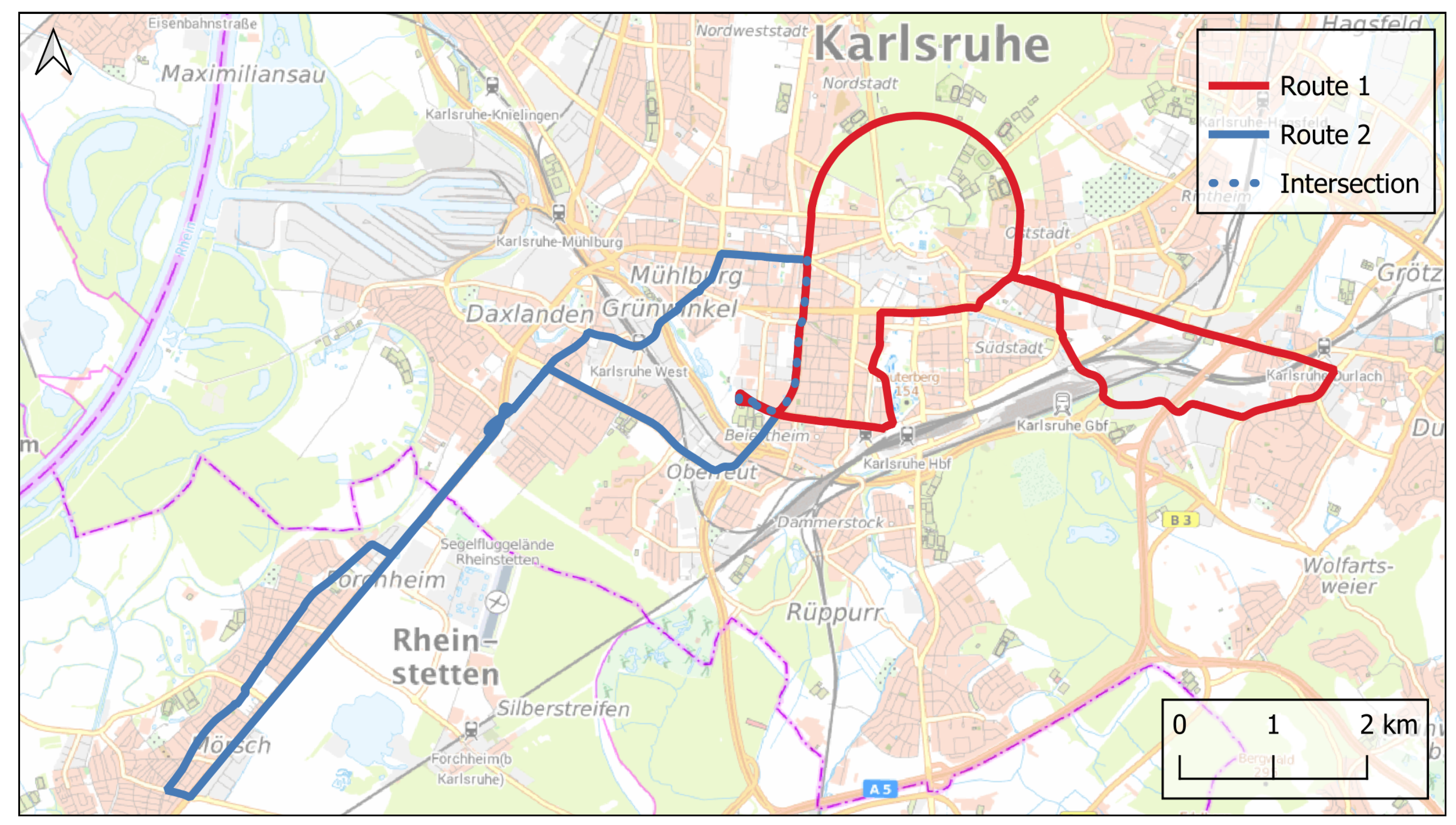
2.1. Study Area in Karlsruhe, Germany—Training Data to Build the Model

Karlsruhe is located in the Upper Rhine Rift Valley, one of the warmest regions in the southwest of Germany (Figure 1).

The city center is located at $49.0$ ${}^{\circ }$ N and $8.4$ ${}^{\circ }$ E at an altitude of approximately 115 $\mathrm{m}$ above the mean sea level. The regional climate of Baden-Württemberg is characterized by a number of extreme meteorological events such as heat waves and heavy thunderstorms due to its exposed location [58,59]. The Upper Rhine Rift Valley has specific climatic conditions, such as high air temperatures and low wind speeds due to the wind shading by the adjacent mountain ridges [60]. These result in warm and humid air and high solar radiation combined with low wind speeds, reflecting the Köppen–Geiger class Cfb for a warm temperate climate [61]. In 2019, 312,060 inhabitants lived in an area of $173.5$ $\mathrm{k}$$\mathrm{m}$${}^2$ ( 1798 inhabitants/$\mathrm{k}$$\mathrm{m}$${}^2$) in Karlsruhe [62]. In 2003, the German air temperature record of $40.2$ ${}^{\circ }\mathrm{C}$, valid until 2015, was recorded at the meteorological station in Karlsruhe. Also, in terms of global climate change, air temperature, summer days, hot days, and tropical nights (under RCP2.6-RCP8.5) are expected to increase by the end of the 21st century [63].

2.2. Study Area in Freiburg, Germany—Test Data to Validate the Model

The city of Freiburg is located in southwestern Germany at $47.6$ ${}^{\circ }$ N, $7.5$ ${}^{\circ }$ E in the Upper Rhine Rift Valley (Figure 2).

With approximately 230,000 inhabitants (as of 2021) and an area of $153.4$ $\mathrm{k}$$\mathrm{m}$${}^2$, it is the third-largest city in the federal state of Baden-Württemberg following Stuttgart and Karlsruhe [64]. The city is located at 278 $\mathrm{m}$ above the mean sea level. The annual average air temperature is $11.5$ ${}^{\circ }\mathrm{C}$ and the average precipitation is $934.0$ $\mathrm{m}$$\mathrm{m}$ [65,66]. To the east of the city center, there is the Schlossberg, a tree-covered hill. In addition, the Dreisam river flows through the city from the southeast of the city center to the northwest end of the city. In terms of parks, Freiburg has several smaller parks in the city center, but two larger green areas are the Hauptfriedhof (main cemetery) in the northern part of the city and the Seepark in the northwest of Freiburg, which also includes a lake. A special feature of Freiburg is the Höllentäler, a mountain–valley wind system that occurs at night and brings cooler air from the east into the city [67]. This wind occurs at night and comes from the Dreisam valley in the east of the city and ventilates the city center. For this analysis, this study was limited to the city center, the city districts of Freiburg, and the adjacent areas such as open fields and forests. The total study area is $41.7$ $\mathrm{k}$$\mathrm{m}$${}^2$. The air temperature, summer days, hot days, and tropical nights are expected to increase by the end of the 21st century (under RCP2.6-RCP8.5) [68].

For the later comparison of the model forecast, mobile measurement data from Freiburg were used. These measurement data were collected with the MeteoBike system and then spatially interpolated and aggregated over several days (Figure 3) [69].

2.3. Processing of Normalized Observational Data from Spatial Neighborhood Analysis for Modeling

In the years 2019 and 2020, 52 measurement runs were spread over two routes with an average duration of 20 min in Karlsruhe (Figure 4) [54]. All measurement runs in 2019 and 2020 took place in June, with calm wind and no clouds on hot summer days. The measuring instruments used rehearsed the route at 1 Hz resulting in different densities of the observations due to different driving speeds. Descriptive statistics for the observations of the air temperature in 2 $\mathrm{m}$ are given in

Table 1. Descriptive statistics for the observations of air temperature in 2 $\mathrm{m}$ AGL in Karlsruhe in 2019.

Time (LT)	Time (UTC)	Min (°C)	Mean (°C)	Max (°C)
0–6	22–4	13.9	18.3	22.0
6–12	4–10	19.5	23.3	28.7
12–18	10–16	26.3	29.4	33.1
18–24	16–22	18.9	25.1	29.3

and

Table 2. Descriptive statistics for the observations of air temperature in 2 $\mathrm{m}$ AGL in Karlsruhe in 2020.

Time (LT)	Time (UTC)	Min (°C)	Mean (°C)	Max (°C)
0–6	22–4	12.3	17.8	21.7
6–12	4–10	19.4	23.7	27.6
12–18	10–16	26.4	28.5	31.3
18–24	16–22	17.2	24.4	29.5

for the years 2019 and 2020, respectively.

The mobile data from the measurement runs ($p_{obs}$) were each initially filtered, and then related to the nearest official meteorological station ($p_{station}$) (Equation (1)), min–max normalized (Equation (2)), and spatially aggregated to create one standardized dataset for each of four time intervals (00:00–06:00; 06:00–12:00; 12:00–18:00; 18:00–24:00 local time (LT)). After this pre-processing, each of these four datasets consisted of 7597 data points with a regular spacing of 5 $\mathrm{m}$ and included the normalized air temperature and further urban covariates [54].

The pre-processing started with the filtering of outliers that were smaller or larger than three times the standard deviation of the raw data. This was followed by filtering according to the wind speed, whereby the observations were filtered out if the wind speed of the nearest official meteorological station was <$0.5$ $\mathrm{m}$/${\mathrm{s}}^{-1}$ or > 3 $\mathrm{m}$/${\mathrm{s}}^{-1}$.

$$p_{rel}=p_{obs}-p_{station}\hspace{1em}\hspace{1em}\hspace{1em}\hspace{1em}\hspace{1em}\hspace{1em}\hspace{1em}\hspace{1em}\hspace{1em}\hspace{1em}\hspace{1em}\left[unit\right(pobs\left)\right]$$

(1)

$$p_{norm}={\displaystyle \frac{p_{rel}-min\left(p_{rel}\right)}{max\left(p_{rel}\right)-min\left(p_{rel}\right)}\hspace{1em}\hspace{1em}\hspace{1em}\hspace{1em}\hspace{1em}\hspace{1em}\hspace{1em}\hspace{1em}\hspace{1em}[0,1]}$$

(2)

The min–max normalization transformed each filtered measurement run from the Celsius scale (${}^{\circ }\mathrm{C}$) to the dimensionless scale [0, 1]. As the measurement routes were driven several times per time interval, several normalized datasets were available for each time interval. The measurements were spatially referenced via Global Positioning System (GPS), which meant that the measurement points of the individual measurement runs were not congruent. The positioning in street canyons deviated on average by 9 $\mathrm{m}$ from the streets of OpenStreetMap (OSM). To obtain a uniform dataset, the normalized measurement runs were spatially aggregated (mean and median) according to the OSM roads with 5 $\mathrm{m}$ spacing. This spatial aggregation per time interval transferred the measurements from a temporal resolution (1 Hz) to a spatial resolution ( 1 $\mathrm{observation}$/5 $\mathrm{m}$). At the same time, the number of measurement runs was reduced due to the aggregation, resulting in a total of four normalized aggregated datasets from 52 measurement runs.

Technically, the software environment for statistical computations R version 4.2.0 and the open source GIS systems System for Automated Geoscientific Analyses (SAGA) and Quantum GIS-3.30 (QGIS) were applied for filtering, normalization, and spatial aggregation [70,71].

These pre-processed datasets are used in this study to train four different GAMs, one per each time interval. The main idea of this study was to explain and model the observed and normalized air temperature by the descriptors of the urban morphology.

2.4. Preparation and Pre-Processing of Descriptors for Modeling and Prediction

At the beginning of this study, many different descriptors were available to describe the urban environment (administrative and remotely sensed). The predictors were classified in the following tables for administrative geodata for the built-up environment (

Table 3. List of available administrative geodata describing the built-up conditions. All datasets were resampled to 10 $\mathrm{m}$ spatial resolution.

Name	Description
Buildings_Official_Dens	Density of buildings within 25 $\mathrm{m}$ and within $0.1$ $\mathrm{k}$$\mathrm{m}$${}^2$ with a radius of 178 $\mathrm{m}$—Buildings are provided by the municipality
Buildings_OSM_Dens	Density of buildings within 25 $\mathrm{m}$ and within $0.1$ $\mathrm{k}$$\mathrm{m}$${}^2$ with a radius of 178 $\mathrm{m}$—Buildings are provided by OpenStreetMap
BuildingHeights_Official_Dens	Density of building heights within 25 $\mathrm{m}$ and within $0.1$ $\mathrm{k}$$\mathrm{m}$${}^2$ with a radius of 178 $\mathrm{m}$

) for UA 2018 classes for land use assessment (

Table 4. List of selected and available Urban Atlas descriptors. Only the descriptors that occurred along the original measurement route were selected [54]. The focus was placed in particular on areal predictors (in contrast to streets). All descriptors were resampled to 10 $\mathrm{m}$ spatial resolution.

Name	Description
UA2018_12100_Dens	Density of the industrial, commercial, public, military, and private units within 25 $\mathrm{m}$ and $0.1$ $\mathrm{k}$$\mathrm{m}$${}^2$
UA2018_14100_Dens	Density of the urban green space within 25 $\mathrm{m}$ and $0.1$ $\mathrm{k}$$\mathrm{m}$${}^2$
UA2018_14200_Dens	Density within 25 $\mathrm{m}$ and $0.1$ $\mathrm{k}$$\mathrm{m}$${}^2$
UA2018_21000_Dens	Density of the arable land (annual crop) within 25 $\mathrm{m}$ and $0.1$ $\mathrm{k}$$\mathrm{m}$${}^2$
UA2018_31000_Dens	Density of the forests within 25 $\mathrm{m}$ and $0.1$ $\mathrm{k}$$\mathrm{m}$${}^2$
UA2018_50000_Dens	Density of water bodies within 25 $\mathrm{m}$ and $0.1$ $\mathrm{k}$$\mathrm{m}$${}^2$
UA2018_12210_Dens	Density of fast transit roads and associated land within 25 $\mathrm{m}$ and $0.1$ $\mathrm{k}$$\mathrm{m}$${}^2$
UA2018_12230_Dens	Density of railways and associated land within 25 $\mathrm{m}$ and $0.1$ $\mathrm{k}$$\mathrm{m}$${}^2$

), as well as further remotely sensed data covering vegetation and sealing (

Table 5. List of available remotely sensed descriptors.

Name	Description	Resolution
NDVI_MEDIAN_2020	Median NDVI derived from Google Earth Engine by [72] based on Landsat 8 data	15 $\mathrm{m}$ (pan-sharpened)
IMD_2018_010m	IMD by Copernicus program [38]	10 $\mathrm{m}$
TCD_2018_010m	TCD by Copernicus program [38]	10 $\mathrm{m}$

).

The UA 2018 classes, the high-resolution layers for imperviousness density (IMD), and TCD were provided by [38]. The official buildings (and their heights) originate from the municipality of Karlsruhe, but additional buildings by OSM were also considered in the model [73]. NDVI was calculated from Landsat 8 data based on the Google Earth Engine script by [72]. The resulting NDVI originally had a resolution of 30 $\mathrm{m}$ but was sharpened by PAN-sharpening to 15 $\mathrm{m}$ and later resampled to 10 $\mathrm{m}$ to align the spatial resolutions of all descriptors. PAN-sharpening was performed with QGIS based on the NDVI output of [72] and the gray bands of Landsat 8. A total of 53 gridded datasets for NDVI and LST were calculated for the summer months from 1 June to 30 September during the period 2016–2020. The resulting gridded datasets were then aggregated (mean and median). NDVI was then used to train the GAMs and LST was used for further validation (Figure A4). The NDVI and LST maps were derived from Landsat 8 imagery with an overpass time of 12:20 LT.

In order to consider the spatial effect, the density of all descriptors was calculated for radii of 25 $\mathrm{m}$ and 178 $\mathrm{m}$ ( $0.1$ $\mathrm{k}$$\mathrm{m}$${}^2$) by SAGA GIS-7.8.2 simple filter function [70]. The densities were calculated to incorporate two different aspects in the subsequent model. On the one hand, the distance to the urban structure (e.g., park, forest, or water body) should be included. On the other hand, the quality and the size of the structure should be included as well (e.g., small park vs. large park or area of dry grass vs. area of irrigated grass). This was also the reason why the density for two radii was calculated −25 $\mathrm{m}$ to assess the microscale effects; and 178 $\mathrm{m}$ to cover the mesoscale effects and to include the size of the structure. Subsequent geoprocessing (cropping to the study area and resampling to 10 $\mathrm{m}$) was applied by QGIS [71]. All predictors were resampled to 10 $\mathrm{m}$ to obtain a uniform grid and a comparable order of magnitude to the air temperature measurements. However, the spatial resolution of some predictors was lower (Table 5) or not provided due to the vector data format (Table 3 and Table 4).

A selection of all descriptors was carried out in order to find the optimal GAM. The requirements for the selection included that the predictors must be independent and available for the whole study area. Principal component analysis (PCA) was applied to the urban morphology descriptors to reduce the number of descriptors and to find the most important principal components (PCs). Later on, the PCs were used to train different GAMs. The whole process is shown in Figure 5.

The descriptors of the lists (Table 3 and Table 4) were applied to the PCA. The PCA resulted in five main PCs describing the thermal regime of the urban environment. The PCA was used to improve the quality of the later model and to reduce intercorrelation among the descriptors.

2.5. Spatial Neighborhood Modeling with Generalized Additive Models

The processed, observed data were related to the neighborhood’s descriptors using GAMs. Compared to a normal linear model (e.g., generalized linear model (GLM)), a GAM replaces the assumption of linearity with a sum of smooth continuous functions for each descriptor [55] (Equation (3)):

$$g\left(E\left(Y\right)\right)={\beta }_0+f_1\left(x_1\right)+f_2\left(x_2\right)+\dots +f_m\left(x_m\right),$$

(3)

A model (mgcv :: bam) was built for each time period (0–6, 6–12, 12–18, and 18–24 LT) and applied to both study areas. The models were trained based on mobile observations, and spatially predicted the UHI. This definition of the model represents the main idea of this study. The computations were conducted with mgcv :: bam instead of mgcv :: gam to allow for the fast parallel computation on the HPC. Each model related the normalized $T_a$ at 2 $\mathrm{m}$ to the descriptors of the neighborhood (in terms of PCs) which correspond to the predictors of the model (Listing 1). The PCs were linked as thin-plate splines with shrinkage ("ts"). The initial basis of each spline was set to k <- 128, but due to automatic shrinkage, all splines shrunk.

Listing 1. GAMs linking normalized Ta at 2 m and PCs to describe the adjacent neighborhood. The models were trained based on mobile observations, and spatially predicted the UHI. This definition of the model represents the main idea of this study.

The models were used to predict the normalized $T_a$ at 2 $\mathrm{m}$ for the entire study area of Karlsruhe and Freiburg, as all predictors were spatially available. One model was built for each time period and applied separately for each prediction. Each model was constructed with the aid of R-4.2.0 and the mgcv package in particular [74].

2.6. Model Selection

The $AIC$ and the $BIC$ were used to select and quantify the quality of each model. The $AIC$ was calculated according to the following Equation (4).

$$AIC=2·k-2·ln\left(\widehat{L}\right),$$

(4)

$ln\left(\widehat{L}\right)$ represents the natural logarithm of the maximum likelihood estimate of the model and k is the number of estimated parameters in the model. $AIC$ rates models with lower values as better. It combines the goodness of fit of the model (through the first term) with a penalty term for model complexity (through the second term). By adding $2·k$ to the first term, the number of parameters in the model is taken into account. The model with the lowest $AIC$ value was selected.

In addition, $BIC$ was applied to the model to obtain a simple model with a small number of descriptors to reduce the overfitting of the model (Equation (5)).

$$BIC=k·ln\left(n\right)-2·ln\left(\widehat{L}\right),$$

(5)

In addition to the number of parameters (k), $BIC$ also takes into account the number of observations (n) and, just like the $AIC$, the natural logarithm of the maximum likelihood estimate of the model ($ln\widehat{L}$).

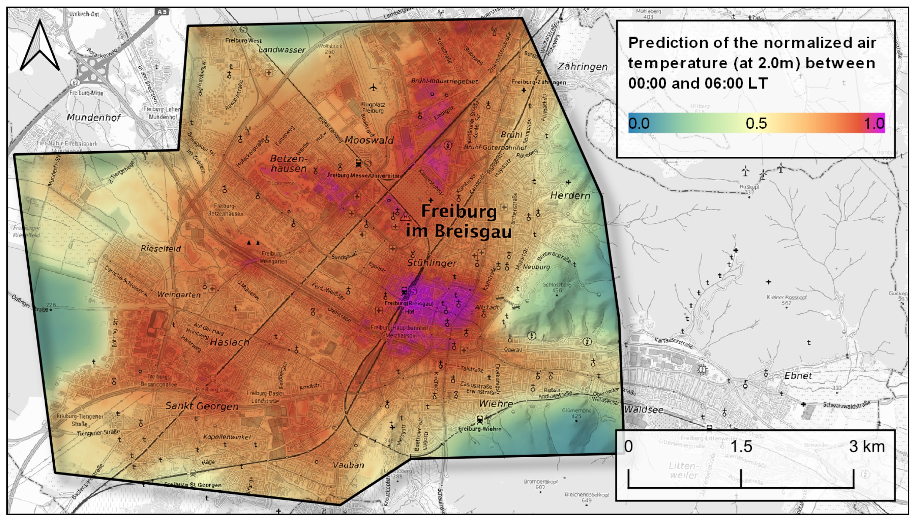
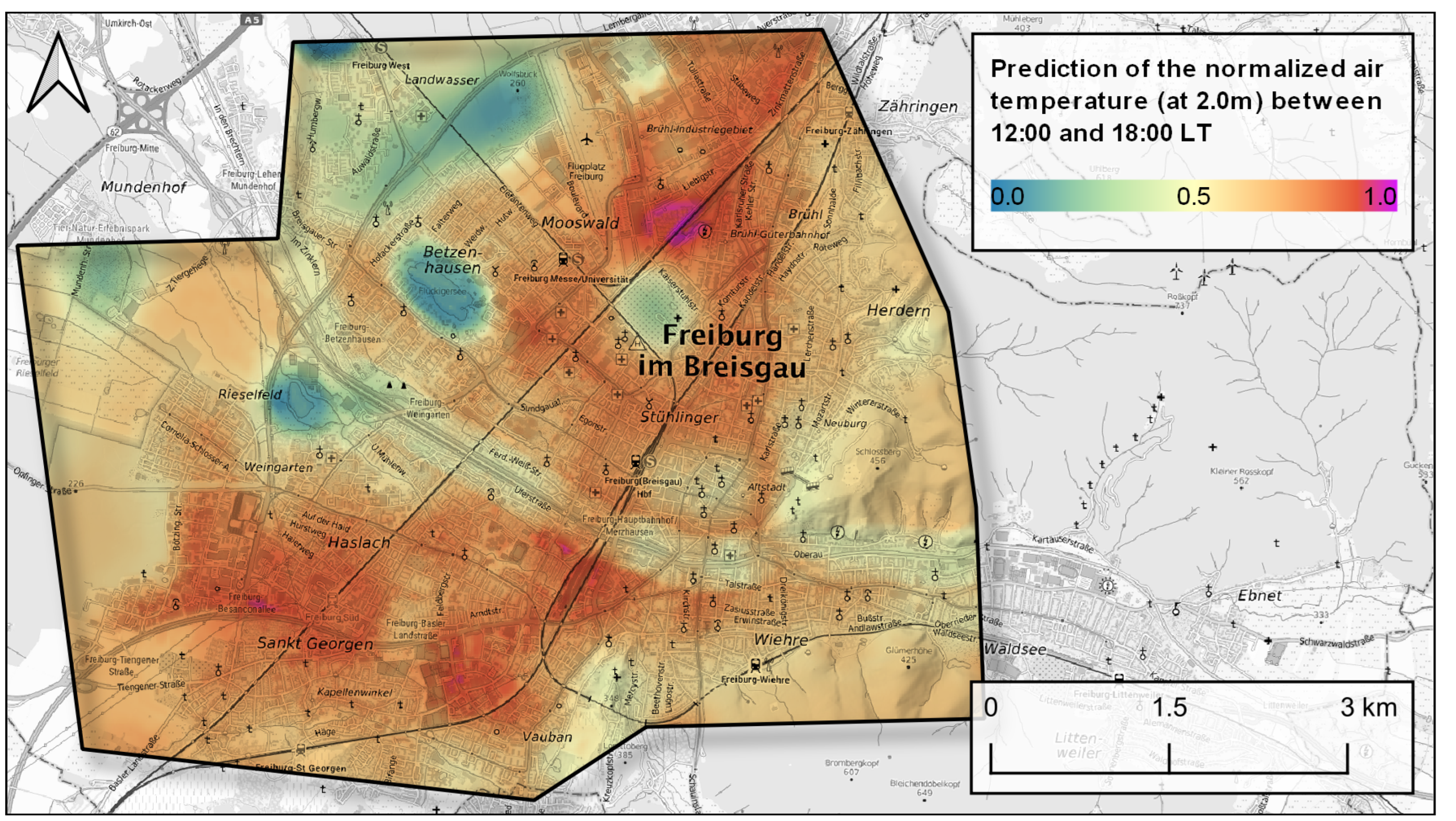
2.7. Validation and Application in Freiburg, Germany

In addition to Karlsruhe, the model was applied to the city of Freiburg. The result was then statistically compared with separate observations. The prediction of the model was compared with the spatial interpolation of mobile measurements which were observed in Freiburg during autochthonous weather conditions. The spatial interpolation was performed using IDW, nearest neighbor (NN), and Kriging methods. IDW gave the best results and was used for further comparison with the GAM. Unfortunately, the comparison of the GAM with the measured data can only be carried out for the period of 18:00–24:00 because the measurements in Freiburg only covered this time period. However, this was also the time when the UHI was most pronounced (

Table 6. List of quality measures for all generated GAMs. Coefficient of determination ($R^2$) is related to the model output and the original observations. The quality of the models was best during the night, and worst during the day.

Time Interval of GAM (LT)	$\mathit{A}\mathit{I}\mathit{C}$	$\mathit{B}\mathit{I}\mathit{C}$	${\mathit{R}}^2$
00:00–06:00	−12,361	−12,314	$75.9$
06:00–12:00	−6607	−6564	$37.7$
12:00–18:00	−8013	−7960	$17.4$
18:00–24:00	−13,380	−13,355	$76.5$

).

The following error measures were used:

• Mean error
  The mean error ($ME$) measures the error between the modeled and the observed value [75]. The following equation was applied:

  $$ME={\displaystyle \frac{1}{N}}\sum _{i=1}^N(S_i-O_i)$$

  (6)

  with N being the number of observations, $S_i$ being the modeled value, and $O_i$ being the observed value.
• Root mean square error
  The $RMSE$ is a measure of accuracy and gives the standard deviation of the model prediction error. This indicates how concentrated the samples are around the best-fitted curve [75]. Smaller values indicate a better model performance.
  The following equation was applied:

  $$RMSE=\sqrt{{\displaystyle \frac{1}{N}}\sum _{i=1}^N{(S_i-O_i)}^2}$$

  (7)

  with N being the number of observations, $S_i$ being the modeled value, and $O_i$ being the observed value.
• Percent bias
  The average tendency of the modeled values to be larger or smaller than the measured values is given by the percent bias ($PBIAS$). Negative values indicate an underestimation bias, positive values indicate an overestimation bias [75]. The bias is expressed in percentage and calculated using the following formula:

  $$PBIAS=100.0·\frac{{\displaystyle \sum _{i=1}^N}(S_i-O_i)}{{\displaystyle \sum _{i=1}^N}{O}_i}$$

  (8)

  with N being the number of observations, $S_i$ being the modeled value, and $O_i$ being the observed value.

In addition to the comparison with another independent model domain, it is also useful to compare the modeled spatial pattern of the normalized UHI (based on $T_a$) with the spatial pattern of the LST. For this purpose, the mean intensity of the S-UHI was calculated for Karlsruhe based on the Google Earth Engine Script by [72]. The script was first used to calculate 53 raster datasets of LST for the summer months of 1 June to 30 September for the years 2016–2020. The satellite images were automatically selected by the script according to cloud cover. Finally, the 53 raster datasets were aggregated with QGIS (mean and median).

3. Results

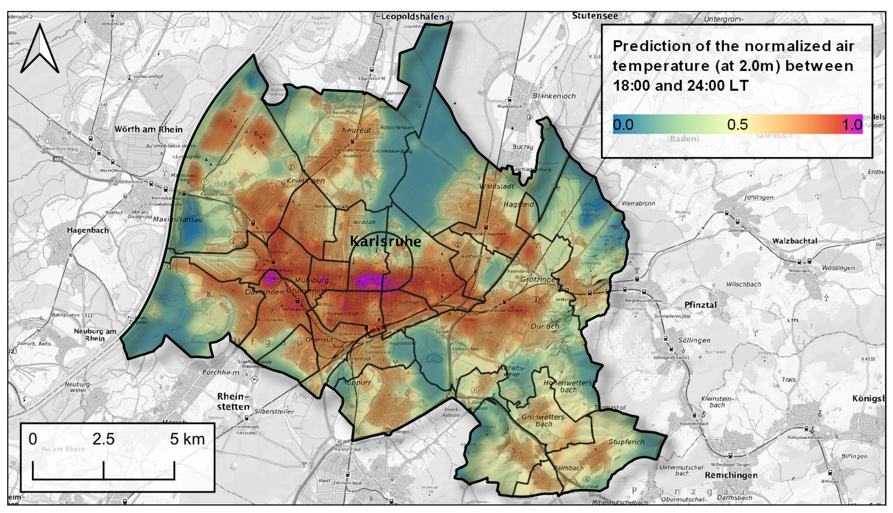
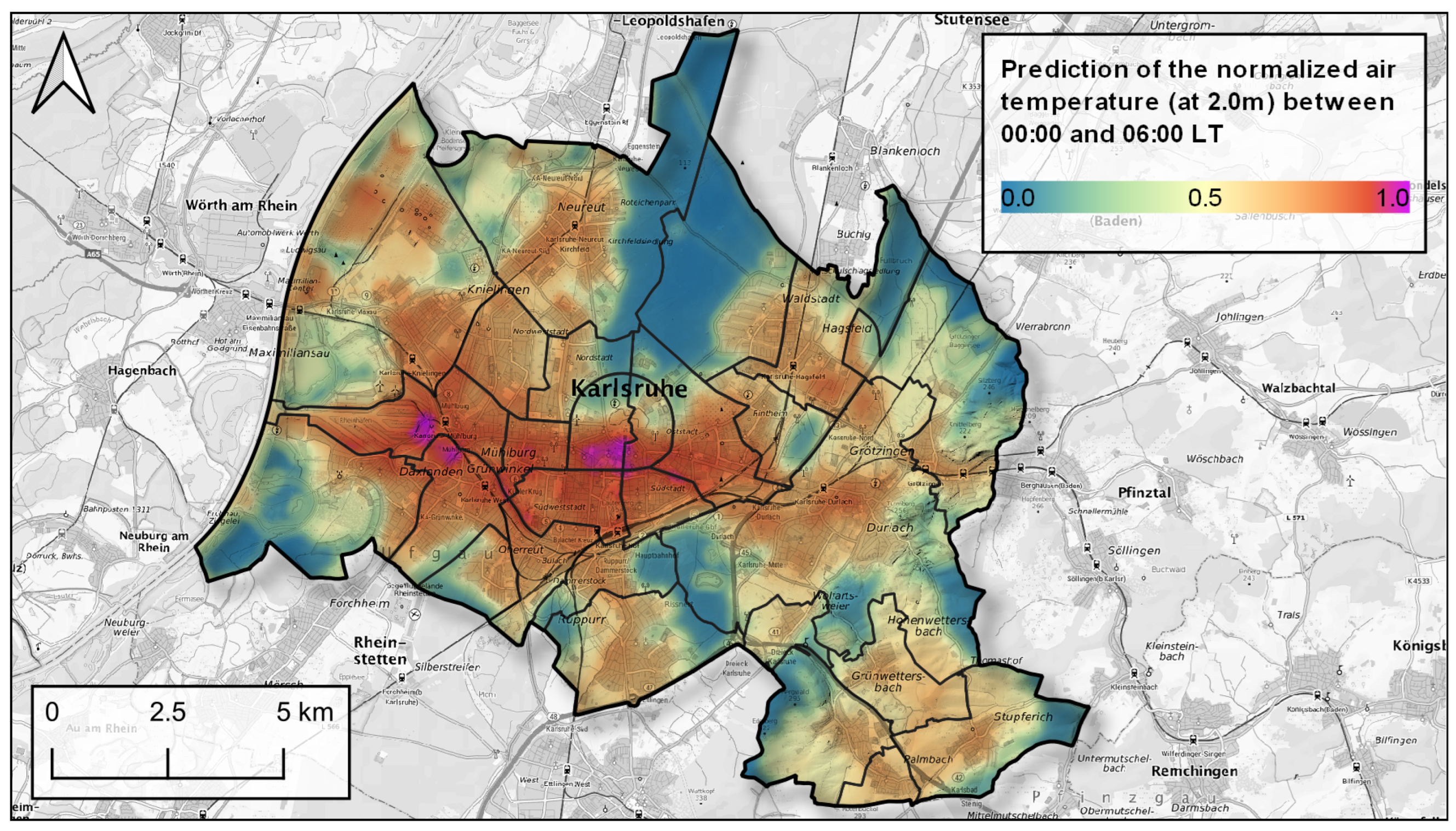
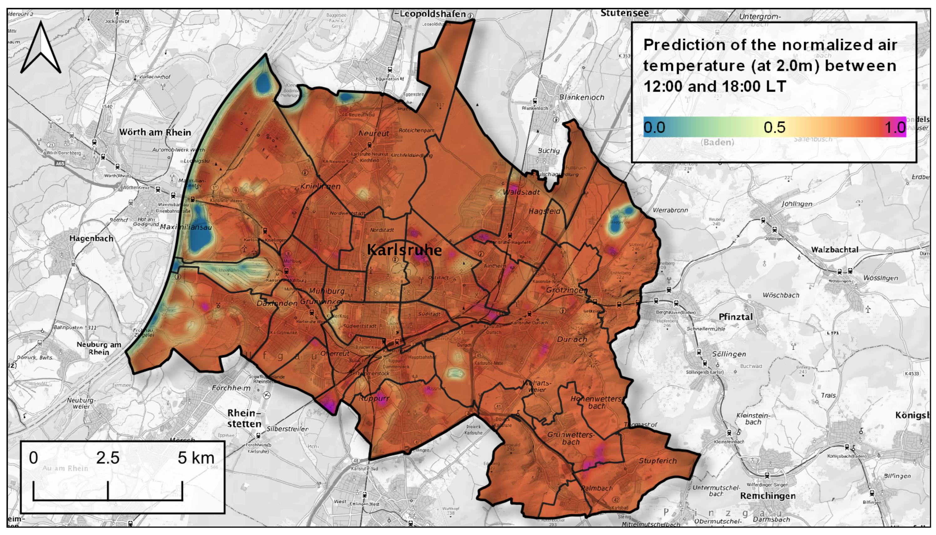
3.1. Spatial Prediction of the Urban Heat Island on the Normalized Scale

The spatial UHI pattern of Karlsruhe was predicted throughout the whole study area based on different descriptors (Listing 1). The spatial prediction for the evening conditions (18–24 LT) showed the spatial heterogeneity of the UHI due to the cooling effects of urban vegetation and the heating effects of sealing (Figure 6).

The evening UHI effect was most pronounced and clearly observable. The map showed the UHI on the normalized scale; the range of the data was transformed to min and max of 0 and 1, respectively. The hot spots of the UHI were located in the city center (e.g., Marketplace and Palace) and the industrial area Grünwinkel in the western part of the city. The cool spots of the city were located in the urban parks (e.g., Günther-Klotz-Anlage, Zoologischer Stadtgarten, Alter Flugplatz, main cemetery and along Albbach River, while the coldest area was found in the urban forest Hardtwald. The hot and cold spots were caused due to the cooling effects of urban vegetation and the heating effects caused by sealed surfaces. Besides Karlsruhe, one could also observe that the smaller towns and villages around Karlsruhe formed their own small UHI.

The results for the morning and midday conditions are shown in Figure A1, Figure A2 and Figure A3. In Figure A1, the impact of urban vegetation is limited due to limited global radiation. With increasing global radiation, the radiation related processes within the city are intensifying. The cooling effect of water bodies, as well as transpirational cooling, is especially evident in Figure A2.

The proposed model for the evening condition was the best among the others. The model for the afternoon prediction had the worst performance and accuracy in terms of $AIC$, $BIC$ and $R^2$ (Table 6). The structure of the UHI pattern was not observed, as no difference between urban and rural areas was visible in the afternoon. But the cooling effect by water bodies was distinctive (Figure A3).

Smaller $AIC$ and $BIC$ indicate better models with fewer parameters and improved generalizability, while higher values of $R^2$ indicate better models with an improved prediction accuracy. Additional information on the individual models regarding F-statistics are listed in

Table A1. Approximative significance of smooth terms for the time interval of 00:00–06:00 LT.

Smooth-Term	k-Index	${\mathit{\chi }}^2$	p-Value
s(PC1)	0.80	189.7	$<2\times {10}^{-16}$
s(PC2)	0.76	2.0	0.0877
s(PC3)	0.79	18.0	$9.82\times {10}^{-6}$
s(PC4)	0.78	2.0	0.0815
s(PC5)	0.81	20.1	$2.2\times {10}^{-6}$

,

Table A2. Approximative significance of smooth terms for the time interval of 06:00–12:00 LT.

Smooth-Term	k-Index	${\mathit{\chi }}^2$	p-Value
s(PC1)	0.74	58.2	$<2\times {10}^{-16}$
s(PC2)	0.76	7.1	0.0043
s(PC3)	0.83	3.2	0.0358
s(PC4)	0.79	5.9	0.0078
s(PC5)	0.77	31.3	$<2\times {10}^{-16}$

, Table A2 and

Table A4. Approximative significance of smooth terms for the time interval 18:00–24:00 LT.

Smooth-Term	k-Index	${\mathit{\chi }}^2$	p-Value
s(PC1)	0.80	215.0	$<2\times {10}^{-16}$
s(PC2)	0.70	0.0	0.6450
s(PC3)	0.77	0.0	0.6610
s(PC4)	0.75	0.0	0.3590
s(PC5)	0.77	23.5	$1.17\times {10}^{-6}$

.

It appeared that the influence of urban parks (e.g., Günther-Klotz-Anlage, Zoologischer Stadtgarten, Hardtwald) had different effects on the normalized air temperature during the day. The impact was enforced during the day, while it was almost absent during the night after midnight. In any case, the maps showed the importance of urban green spaces and urban forests in reducing the thermal load in inner-city areas. On the other hand, it can be seen that completely sealed areas (e.g., Industrial area Grünwinkel and Industrial area Oststadt—without green roofs) heated up the most and also contributed the most to the formation of the UHI.

3.2. Validation and Error of the Model Output

The developed models were applied to a second study area as described in Section 2 to prove and demonstrate the generalizability and transferability of the model. The prediction for the city of Freiburg showed a reasonable typical formation of the UHI with hot spots in the core of the city and in the industrial areas in the southwest and northeast of Freiburg (Figure 7).

The cold spots, according to the model, were areas with urban green space and areas in the outskirts of the city. In particular, these were the main cemetery (Hauptfriedhof), local recreation areas (Seepark), and allotment gardens. Multiple hot spots were observed in industrial areas (e.g., Gewerbegebiet Haid and Industriegebiet Nord) as well as in the city center. The pattern also included a gradient from the city center to the rural areas.

The spatial differences between the model output for 18:00–24:00 LT and the reference dataset differed especially in terms of the topographically characterized regions (Schlossberg) as well as in the areas with flowing water and water bodies (Dreisam River) (Figure 8).

The spatial model output for the other time periods is shown in Figure A5, Figure A6 and Figure A7. The cooling effect by urban parks during the night (Figure A5) was limited in comparison to daytime predictions (Figure A7). In contrast to nighttime conditions, the cooling effect by urban parks (e.g., in main cemetery, Seepark, and Dietenbachpark) was observed in the morning hours (Figure A6). The main hot spot was located in the industrial area in the north. The model for the daytime prediction had the worst performance and accuracy (Figure A7). The structure of the UHI pattern was mainly modified by water bodies and buildings. The cooling effect by urban parks was reinforced in comparison to the nighttime conditions.

The statistical validation could only be performed for the time period 18:00–24:00 LT because the mobile measurement data from MeteoBikes in Freiburg were only available for this time period. Based on the prediction of the GAMs and the interpolated mobile measurements, the quality measures ($ME$, $RMSE$ and $PBIAS$) were calculated for the evening conditions (18:00–22:00 LT) (

Table 7. List of error measures for the prediction of the evening conditions, including $ME$, $RMSE$, and $PBIAS$. All measures compared the model output (Figure 7) with the interpolated observations (Figure 3).

ME	RMSE	PBIAS	R2
0.03	0.12	$4.6$	$69.0$

).

The link between the GAM output of the evening condition in relation to the observations in Freiburg are depicted in Figure 9.

The point cloud of this linear regression was based on both raster datasets (each point represents one pixel of the model and the observation). The model and the observations were highly linearly correlated, with a coefficient of determination of 0.69. In addition, it was observed that the model and observations agreed the best for higher values and differed for lower values. This means that the model performed better in urban than rural areas. At the same time, this also showed the heteroscedasticity (the heterogenicity of the variance) in the data, which should be further investigated in the future.

In addition to applying the model to another model area, the modeled normalized UHI (based on $T_a$) can be compared with the observed S-UHI in Karlsruhe (Figure A4).

4. Discussion

The model has some limitations regarding the missing coverage of specific land covers. For example, the model was not explicitly trained on water bodies. Furthermore, the model was not trained on regions with distinctive elevation and underlying local meteorological effects (sea breeze, mountain breeze and valley breeze, cold airflow). Data on the anthropogenic heat release and soil moisture were also not incorporated and were therefore not considered. But, in comparison with interpolated, mobile measurements in Freiburg, it was shown that the model is suitable for predicting the normalized pattern of the UHI for comparable mid-latitude cities. The output is static and independent of the prevailing weather and local spatial influences, and yet the model can provide valuable information for long-term urban planning. This is particularly evident in the visual comparison of the modeled UHI with the observed S-UHI from remotely sensed LST-data (Figure 6 and Figure A4).

It is based on GAMs, while others have applied various statistical or ML algorithms (e.g., RandomForest or Tensorflow) [27]. In the future, new methods such as NN can be considered [76]. However, this may require additional measurement runs and data.

The model is not yet sufficient for human-biometeorological analyses, as information on the radiation budget, humidity, wind speed, and win direction are missing. In the future, the model could perhaps be compared directly with a PET—which would have to be derived from the aforementioned variables [77,78]. Unfortunately, wind speed was not available from the mobile measurements. The mobile measurements of wind speed are, in general, quite difficult to obtain, because of the turbulence caused by the surroundings and different driving speeds of the car in the city [79].

Determining the radiation budget poses also a challenge, since shading depends on small-scale structures. For example, the choice of the roadway during mobile measurements influenced the observation of global radiation due to shading. Cooling by transpiration and shading is related to global radiation, in particular to photosynthetically active radiation (PAR). PAR is absent during the night, resulting in the limited stomatal conductance of the leaves [80]. Therefore, cooling by transpiration cannot be observed because transpiration is limited by closed stomata [44,81]. Cooling by shading was also absent due to the absence of global radiation. At night, cooling mainly occurs due to the emission of longwave (thermal) radiation from black (or better gray) bodies with prevailing surface temperature. Alternatively, the SVF could be included in the model as an additional descriptor. SVF is a metric used to quantify the proportion of visible sky from a point on the ground. It provides information about the openness and visibility of the sky in the urban environment. SVF can be obtained from numerical models (e.g., SkyHelios or RayMan), and directly influences PET because of mean radiant temperature (T_mrt) [82]. Unfortunately, the calculation of SVF for the entire urban area was not possible either, as the model area was too large for this. Furthermore, SVF can only be calculated for areas, for which the necessary morphological data are available (e.g., which is possible for inner-city areas; but not for the Hardtwald), which is why SVF was not added to the model as an additional descriptor. In addition, it was also shown that T_mrt can also be assessed by deep convolutional encoder–decoder, without the need to run computationally expensive models [83]. On the other hand, additional data would be needed for the spatial, three-dimensional resolution of small-scale structures within the city. For example, 3D light detecting and ranging (LIDAR) data could provide additional information about individual tree canopies and surfaces as digital twins in general [84,85,86].

Unfortunately, the comparison of the spatial interpolation of Freiburg with the prediction for Freiburg was also subject to errors because the spatial IDW interpolation itself contained errors. In particular, the spatial interpolation was based on measurements made with a different measuring system (measurement cart of German meteorological service (DWD) and MeteoBike). However, care was taken to ensure that the meteorological conditions were similar (autochthonous weather conditions with a low wind speed), and the goal was to model the physical quantity of air temperature at 2 $\mathrm{m}$ which should have the identical or similar values regardless of the measurement system.

4.1. Missing Coverage of Specific Land Cover

The urban area of Karlsruhe is not strongly topographically shaped (unlike other cities such as Freiburg or Stuttgart) [87,88]. A digital terrain model was integrated into the model, but the combination of the elevation with the observations was not representative because the variance of the altitude in Karlsruhe is not significant. Thus, the topography poses a challenge to the model, which was particularly evident in the validation for Freiburg (Figure 8). The largest errors were found for the topographically shaped Schlossberg (pink). Since the topography is not very important for Karlsruhe itself, the model can still be applied to Karlsruhe, but has limitations and implications for topographic cities like Freiburg.

The same is true for water bodies in urban areas. The mobile measurements passed by a quarry pond, but not directly along flowing water bodies such as the Rhine or the Alb. This severely limits the significance of the model in the area of flowing waters, which was also shown by the validation along the Dreisam River (green). Nevertheless, the thermal effects of standing water on the urban atmosphere can be observed (Figure 7 and Figure A5). At night, lakes can be considered as heat sources, as has already been shown by other authors [46,89]. However, the model could be improved by additional measurement runs in topographically dominated areas or near rivers and lakes.

In addition to the aforementioned issues, the model heavily relies on the land use classification of UA 2018. According to [90], the UA 2018 classification has better accuracy than CLC and will therefore lead to more accurate results. The classification according to UA 2018 in Karlsruhe and Freiburg was mostly correct, but some parts were misclassified, which then led to inaccurate predictions by the model in these areas.

4.2. Missing Data on Anthropogenic Heat Production and Soil Moisture

Furthermore, the model is missing data on soil moisture and water availability to urban trees. Soil moisture has a large influence on the cooling potential through transpiration. Moreover, these factors change throughout the year and especially during prolonged periods of heat and drought.

Unfortunately, the anthropogenic heat production and emission from individual transportation were also not available in sufficient resolution. With vehicle counts and information on heat-emitting processes in the city, a more accurate map of the UHI in street canyons, in residential areas, and in industrial areas could be obtained. There are some datasets about anthropogenic heat production, but mainly at the city level [91]. Google Environmental Insights Explorer also provides data on individual traffic, but also only at the city level, with incoming and outgoing traffic and not within individual streets [92].

4.3. Concurvity Shows the Dependency of Various Predictors

Concurvity describes the interdependence of multiple descriptors to explain a target variable. It cannot be completely avoided in the model, but has been reduced as much as possible by selecting thin-plate splines with shrinkage and using the selection option in the model. In addition, the descriptors were not directly applied to the GAM, but were analyzed with the PCA as described in Section 2.4. If the concurvity is too severe, the model would become numerically unstable. This was not the case with the presented models.

4.4. Applications and Implications of Spatial UHI Modeling in Resilient Urban Planning, Health Sector, Tourism, and Architecture

The models can be used to assess the UHI with spatial and temporal resolution. In particular, the hot spots in the city represent areas of increased thermal risk. The UHI alone, however, is not sufficient to capture the thermal risk of the urban population. Rather, it is necessary to combine the thermal component with the socioeconomic and infrastructural factors (e.g., age structure, income and wealth, accessibility of urban green spaces, etc.). With this knowledge, urban planners and decision makers can react appropriately and implement local measures to mitigate the UHI. Climate-adapted urban planning increases the quality of life in cities, improves people’s health and productivity, and is responsive to people’s needs [2,93,94]. For example, during the coronavirus pandemic, the desire of urban dwellers for urban green spaces was demonstrated [95]. Climate-adapted urban planning means reducing sealing in the city, creating, maintaining, and where possible, expanding urban green space (UGS). Permeable surfaces (permeable tiles) also contribute to this, as do facade greening and green roofs [8,10,96,97,98,99]. It is particularly important to implement the measures on a large scale to counteract the effects of sealing. In addition, artificial measures should also be considered in places where nature-based solutions are not possible (e.g., water fountains, sources of drinking water, white roofs, and shadow casting infrastructure) [11,46,89]. This can also promote the well-being of people in areas that are characterized by tourism (e.g., drinking water fountains near Karlsruhe Palace or in Freiburg’s old town). Measures that can be controlled depending on the season (e.g., that provide shade in summer and not in winter) would also be ideal. In addition to planning measures, other acute heat protection measures relating to communication and behavioral adaptation are also conceivable. As a result of adapted urban planning, the financial land value of a city can also increase with the increasing UGS and a decline with a lack of UGS [100,101]. If all these implications are addressed, then this also contributes to the objectives of the Sendai Framework for Disaster Risk Reduction and the Sustainable Development Goals for sustainable cities and communities [102,103].

5. Conclusions

The combination of official administrative geospatial data, remotely sensed data, and in situ observations offer great potential to assess the spatial pattern of a city’s UHI or its urban heat archipelago. The model has some limitations in topographically shaped regions, but this could be resolved in the future if the additional measurements and observations of such regions are included in the model. Such data may already be available in scientific data repositories (e.g., Zenodo), but are difficult to use due to different data structures and formats. The derived GAM is generally applicable to cities of similar latitude and character. The model is an additional tool for adapted urban planning and can contribute to the improvement of climate resilience and improved urban planning. Furthermore, it is fast and easy to use, but local conditions, e.g., local wind systems—such as Höllentäler in Freiburg—cannot be resolved because it is a static and not process-based numerical model. However, this was not the intention of the model, as it was mainly designed to analyze the UHI pattern during autochthonous weather conditions with low wind speed. With the help of the model, local microscale heat health warning systems could be developed in the future that consider the local conditions of a city and the thermal risk of the urban environment. In combination with the protective factors (e.g., accessibility of urban green spaces, hospitals, pharmacies, and doctors), vulnerable people could be protected. If the thermal risk (assessed as the UHI) in combination with protective factors is incorporated into urban plans and strategies (HHAP and climate adaptation plans), this information and the actions for UHI mitigation can also be implemented in practice and fulfill the objectives of national and international strategies for UHI mitigation (e.g., Sendai Framework for Disaster Risk Reduction and the Sustainable Development Goals for sustainable cities and communities).

References

1. United Nations, Department of Economic and Social Affairs, Population Division. World Urbanization Prospects: The 2018 Revision; United Nations, Department of Economic and Social Affairs, Population Division: New York, NY, USA, 2019. [Google Scholar]
2. Gehl, J. Cities for People; Island Press: Washington, DC, USA, 2010. [Google Scholar]
3. Węziak-Białowolska, D. Quality of life in cities—Empirical evidence in comparative European perspective. Cities 2016, 58, 87–96. [Google Scholar] [CrossRef]
4. Matzarakis, A. A Note on the Assessment of the Effect of Atmospheric Factors and Components on Humans. Atmosphere 2020, 11, 1283. [Google Scholar] [CrossRef]
5. Revi, A.; Satterthwaite, D.E.; Aragón-Durand, F.; Corfee-Morlot, J.; Kiunsi, R.B.R.; Pelling, M.; Roberts, D.C.; Solecki, W. Urban areas. In Climate Change 2014: Impacts, Adaptation, and Vulnerability. Part A: Global and Sectoral Aspects. Contribution of Working Group II to the Fifth Assessment Report of the Intergovernmental Panel of Climate Change; Field, C.B., Barros, V.R., Dokken, D.J., Mach, K.J., Mastrandrea, M.D., Bilir, T.E., Chatterjee, M., Ebi, K.L., Estrada, Y.O., Genova, R.C., et al., Eds.; Cambridge University Press: Cambridge, UK; New York, NY, USA, 2014; pp. 535–612. [Google Scholar]
6. Masson, V.; Lemonsu, A.; Hidalgo, J.; Voogt, J. Urban Climates and Climate Change. Annu. Rev. Environ. Resour. 2020, 45, 411–444. [Google Scholar] [CrossRef]
7. Zeeshan, M.; Ali, Z. The Potential of Cool Materials Towards Improving Thermal Comfort Conditions Inside Real-urban Hot-humid Microclimate. Environ. Urban. Asia 2022, 13, 56–72. [Google Scholar] [CrossRef]
8. Šenfeldr, M.; Maděra, P.; Kotásková, P.; Fialová, J.; Kundrata, M.; Rieger, V. The Green Roofs and Facades as a Tool of Climate Cooling in the Urban Environment. In Management of Water Quality and Quantity; Zelenakova, M., Hlavínek, P., Negm, A.M., Eds.; Springer International Publishing: Cham, Switzerland, 2020; pp. 39–75. [Google Scholar] [CrossRef]
9. Akbari, H.; Pomerantz, M.; Taha, H. Cool surfaces and shade trees to reduce energy use and improve air quality in urban areas. Sol. Energy 2001, 70, 295–310. [Google Scholar] [CrossRef]
10. Eingrüber, N.; Domm, A.; Korres, W.; Löhnert, U.; Schneider, K. Climate change adaption potentials of unsealing strategies in cities – An assessment during heat and drought events based on microclimatic simulations. In Proceedings of the EMS Anual Meeting 2023, Bratislava, Slovakia, 3–8 September 2023. [Google Scholar] [CrossRef]
11. Wang, L.; Huang, M.; Li, D. Where Are White Roofs More Effective in Cooling the Surface? Geophys. Res. Lett. 2020, 47, e2020GL087853. [Google Scholar] [CrossRef]
12. Masson, V.; Heldens, W.; Bocher, E.; Bonhomme, M.; Bucher, B.; Burmeister, C.; de Munck, C.; Esch, T.; Hidalgo, J.; Kanani-Sühring, F.; et al. City-descriptive input data for urban climate models: Model requirements, data sources and challenges. Urban Clim. 2020, 31, 100536. [Google Scholar] [CrossRef]
13. Sobrino, J.; Oltra-Carrió, R.; Sòria, G.; Bianchi, R.; Paganini, M. Impact of spatial resolution and satellite overpass time on evaluation of the surface urban heat island effects. Remote. Sens. Environ. 2012, 117, 50–56. [Google Scholar] [CrossRef]
14. Voogt, J.A.; Oke, T.R. Effects of urban surface geometry on remotely-sensed surface temperature. Int. J. Remote Sens. 1998, 19, 895–920. [Google Scholar] [CrossRef]
15. Wang, D.; Chen, Y.; Hu, L.; Voogt, J.A.; He, X. Satellite-based daytime urban thermal anisotropy: A comparison of 25 global cities. Remote. Sens. Environ. 2022, 283, 113312. [Google Scholar] [CrossRef]
16. Parsons, K.C. Human Thermal Environments: The Effects of Hot, Moderate, and Cold Environments on Human Health, Comfort, and Performance, 3rd ed.; CRC Press/Taylor & Francis: Boca Raton, FL, USA, 2014. [Google Scholar]
17. Voogt, J.; Oke, T. Thermal remote sensing of urban climates. Remote Sens. Environ. 2003, 86, 370–384. [Google Scholar] [CrossRef]
18. Gallo, K.; Hale, R.; Tarpley, D.; Yu, Y. Evaluation of the Relationship between Air and Land Surface Temperature under Clear- and Cloudy-Sky Conditions. J. Appl. Meteorol. Climatol. 2011, 50, 767–775. [Google Scholar] [CrossRef]
19. Pichierri, M.; Bonafoni, S.; Biondi, R. Satellite air temperature estimation for monitoring the canopy layer heat island of Milan. Remote Sens. Environ. 2012, 127, 130–138. [Google Scholar] [CrossRef]
20. Huang, W.; Li, J.; Guo, Q.; Mansaray, L.; Li, X.; Huang, J. A Satellite-Derived Climatological Analysis of Urban Heat Island over Shanghai during 2000–2013. Remote Sens. 2017, 9, 641. [Google Scholar] [CrossRef]
21. Romero Rodríguez, L.; Sánchez Ramos, J.; Sánchez de la Flor, F.J.; Álvarez Domínguez, S. Analyzing the urban heat Island: Comprehensive methodology for data gathering and optimal design of mobile transects. Sustain. Cities Soc. 2020, 55, 102027. [Google Scholar] [CrossRef]
22. Kotharkar, R.; Surawar, M. Land Use, Land Cover, and Population Density Impact on the Formation of Canopy Urban Heat Islands through Traverse Survey in the Nagpur Urban Area, India. J. Urban Plan. Dev. 2016, 142, 04015003. [Google Scholar] [CrossRef]
23. Saaroni, H.; Ben-Dor, E.; Bitan, A.; Potchter, O. Spatial distribution and microscale characteristics of the urban heat island in Tel-Aviv, Israel. Landsc. Urban Plan. 2000, 48, 1–18. [Google Scholar] [CrossRef]
24. Chandler, T.J. Temperature and Humidity Traverses across London. Weather 1962, 17, 235–242. [Google Scholar] [CrossRef]
25. Straub, A.; Berger, K.; Breitner, S.; Cyrys, J.; Geruschkat, U.; Jacobeit, J.; Kühlbach, B.; Kusch, T.; Philipp, A.; Schneider, A.; et al. Statistical modelling of spatial patterns of the urban heat island intensity in the urban environment of Augsburg, Germany. Urban Clim. 2019, 29, 100491. [Google Scholar] [CrossRef]
26. Shandas, V.; Voelkel, J.; Williams, J.; Hoffman, J. Integrating Satellite and Ground Measurements for Predicting Locations of Extreme Urban Heat. Climate 2019, 7, 5. [Google Scholar] [CrossRef]
27. Voelkel, J.; Shandas, V. Towards Systematic Prediction of Urban Heat Islands: Grounding Measurements, Assessing Modeling Techniques. Climate 2017, 5, 41. [Google Scholar] [CrossRef]
28. Zumwald, M.; Knüsel, B.; Bresch, D.N.; Knutti, R. Mapping urban temperature using crowd-sensing data and machine learning. Urban Clim. 2021, 35, 100739. [Google Scholar] [CrossRef]
29. Zumwald, M.; Baumberger, C.; Bresch, D.N.; Knutti, R. Assessing the representational accuracy of data-driven models: The case of the effect of urban green infrastructure on temperature. Environ. Model. Softw. 2021, 141, 105048. [Google Scholar] [CrossRef]
30. Chen, S.; Yang, Y.; Deng, F.; Zhang, Y.; Liu, D.; Liu, C.; Gao, Z. A high-resolution monitoring approach of canopy urban heat island using a random forest model and multi-platform observations. Atmos. Meas. Tech. 2022, 15, 735–756. [Google Scholar] [CrossRef]
31. Venter, Z.S.; Brousse, O.; Esau, I.; Meier, F. Hyperlocal mapping of urban air temperature using remote sensing and crowdsourced weather data. Remote Sens. Environ. 2020, 242, 111791. [Google Scholar] [CrossRef]
32. Venter, Z.S.; Chakraborty, T.; Lee, X. Crowdsourced air temperatures contrast satellite measures of the urban heat island and its mechanisms. Sci. Adv. 2021, 7, eabb9569. [Google Scholar] [CrossRef] [PubMed]
33. Vulova, S.; Meier, F.; Fenner, D.; Nouri, H.; Kleinschmit, B. Summer Nights in Berlin, Germany: Modeling Air Temperature Spatially With Remote Sensing, Crowdsourced Weather Data, and Machine Learning. IEEE J. Sel. Top. Appl. Earth Obs. Remote Sens. 2020, 13, 5074–5087. [Google Scholar] [CrossRef]
34. Dos Santos, R.S. Estimating spatio-temporal air temperature in London (UK) using machine learning and earth observation satellite data. Int. J. Appl. Earth Obs. Geoinf. 2020, 88, 102066. [Google Scholar] [CrossRef]
35. Fiorillo, E.; Brilli, L.; Carotenuto, F.; Cremonini, L.; Gioli, B.; Giordano, T.; Nardino, M. Diurnal Outdoor Thermal Comfort Mapping through Envi-Met Simulations, Remotely Sensed and In Situ Measurements. Atmosphere 2023, 14, 641. [Google Scholar] [CrossRef]
36. Nardino, M.; Cremonini, L.; Crisci, A.; Georgiadis, T.; Guerri, G.; Morabito, M.; Fiorillo, E. Mapping daytime thermal patterns of Bologna municipality (Italy) during a heatwave: A new methodology for cities adaptation to global climate change. Urban Clim. 2022, 46, 101317. [Google Scholar] [CrossRef]
37. D’Acci, L. (Ed.) The Mathematics of Urban Morphology; Modeling and Simulation in Science, Engineering and Technology Series; Springer International Publishing: Cham, Switzerland, 2019. [Google Scholar] [CrossRef]
38. European Environment Agency (EEA). Copernicus Land Monitoring Service 2018; European Environment Agency: Copenhagen, Denmark, 2018.
39. Stewart, I.D.; Oke, T.R. Local Climate Zones for Urban Temperature Studies. Bull. Am. Meteorol. Soc. 2012, 93, 1879–1900. [Google Scholar] [CrossRef]
40. Oke, T.R. Initial Guidance to Obtain Representative Meteorological Observations at Urban Sites; World Meteorological Organization: Geneva, Switzerland, 2004. [Google Scholar]
41. Keil, M.; Kiefl, R.; Strunz, G. CORINE Land Cover 2000—European-Wide Harmonised Update of Land Use Data for Germany; DLR: Wessling, Germany, 2005. [Google Scholar]
42. Oke, T.R.; Mills, G.; Christen, A.; Voogt, J.A. Urban Climates; Cambridge University Press: Cambridge, UK, 2017. [Google Scholar] [CrossRef]
43. ASHRAE. 2017 ASHRAE Handbook: Fundamentals; ASHRAE: Peachtree Corners, GA, USA, 2017. [Google Scholar]
44. Jones, H.G. Plants and Microclimate: A Quantitative Approach to Environmental Plant Physiology, 3rd ed.; Cambridge University Press: Cambridge, UK, 2013. [Google Scholar] [CrossRef]
45. Ferrini, F.; van den Bosch, C.; Fini, A. (Eds.) Routledge Handbook of Urban Forestry; Routledge/Taylor & Francis: London, UK; New York, NY, USA, 2017. [Google Scholar]
46. Solcerova, A.; van de Ven, F.; van de Giesen, N. Nighttime Cooling of an Urban Pond. Front. Earth Sci. 2019, 7, 156. [Google Scholar] [CrossRef]
47. Toparlar, Y.; Blocken, B.; Maiheu, B.; van Heijst, G. A review on the CFD analysis of urban microclimate. Renew. Sustain. Energy Rev. 2017, 80, 1613–1640. [Google Scholar] [CrossRef]
48. Antoniou, N.; Montazeri, H.; Neophytou, M.; Blocken, B. CFD simulation of urban microclimate: Validation using high-resolution field measurements. Sci. Total Environ. 2019, 695, 133743. [Google Scholar] [CrossRef] [PubMed]
49. Buccolieri, R.; Hang, J. Recent Advances in Urban Ventilation Assessment and Flow Modelling. Atmosphere 2019, 10, 144. [Google Scholar] [CrossRef]
50. Kang, G.; Kim, J.J.; Choi, W. Computational fluid dynamics simulation of tree effects on pedestrian wind comfort in an urban area. Sustain. Cities Soc. 2020, 56, 102086. [Google Scholar] [CrossRef]
51. Lenz, S.; Schönherr, M.; Geier, M.; Krafczyk, M.; Pasquali, A.; Christen, A.; Giometto, M. Towards real-time simulation of turbulent air flow over a resolved urban canopy using the cumulant lattice Boltzmann method on a GPGPU. J. Wind Eng. Ind. Aerodyn. 2019, 189, 151–162. [Google Scholar] [CrossRef]
52. Mortezazadeh, M.; Wang, L.L.; Albettar, M.; Yang, S. CityFFD – City fast fluid dynamics for urban microclimate simulations on graphics processing units. Urban Clim. 2022, 41, 101063. [Google Scholar] [CrossRef]
53. Mortezazadeh, M.; Zou, J.; Hosseini, M.; Yang, S.; Wang, L. Estimating Urban Wind Speeds and Wind Power Potentials Based on Machine Learning with City Fast Fluid Dynamics Training Data. Atmosphere 2022, 13, 214. [Google Scholar] [CrossRef]
54. Gangwisch, M.; Saha, S.; Matzarakis, A. Spatial neighborhood analysis linking urban morphology and green infrastructure to atmospheric conditions in Karlsruhe, Germany. Urban Clim. 2023, 51, 101624. [Google Scholar] [CrossRef]
55. Hastie, T.; Tibshirani, R. Generalized additive models. In Generalized Additive Models, 1st ed.; Routledge: Abingdon-on-Thames, UK, 2017; pp. 136–173. [Google Scholar] [CrossRef]
56. Ravindra, K.; Rattan, P.; Mor, S.; Aggarwal, A.N. Generalized additive models: Building evidence of air pollution, climate change and human health. Environ. Int. 2019, 132, 104987. [Google Scholar] [CrossRef] [PubMed]
57. Bassett, R.; Janes-Bassett, V.; Phillipson, J.; Young, P.; Blair, G. Climate driven trends in London’s urban heat island intensity reconstructed over 70 years using a generalized additive model. Urban Clim. 2021, 40, 100990. [Google Scholar] [CrossRef]
58. Wagner, A. Zukünftige Klimaentwicklungen in Baden-Württemberg: Perspektiven aus Regionalen Klimamodellen, langfassung ed.; Landesanstalt für Umwelt, Messungen und Naturschutz Baden-Württemberg: Karlsruhe, Germany, 2013. [Google Scholar]
59. Gebhardt, H.; Landesanstalt für Umwelt, Messungen und Naturschutz Baden-Württemberg (Eds.) Climate Change in Baden-Württemberg: Facts-Impacts-Perspectives, 2nd updated ed.; Ministry of the Environment, Climate Protection and the Energy Sector: Stuttgart, Germany, 2012. [Google Scholar]
60. Hackenbruch, J. Anpassungsrelevante Klimaänderungen für Städtische Baustrukturen und Wohnquartiere; Number 77 in Wissenschaftliche Berichte des Instituts für Meteorologie und Klimaforschung des Karlsruher Instituts für Technologie; KIT Scientific Publishing: Karlsruhe, Germany, 2018. [Google Scholar]
61. Rubel, F.; Kottek, M. Observed and projected climate shifts 1901-2100 depicted by world maps of the Köppen-Geiger climate classification. Meteorol. Z. 2010, 19, 135–141. [Google Scholar] [CrossRef]
62. Statistisches Landesamt Baden-Württemberg. Bevölkerung, Gebiet und Bevölkerungsdichte. 2020. Available online: https://www.statistik-bw.de/BevoelkGebiet/Bevoelkerung/01515020.tab?R=KR212 (accessed on 18 November 2021).
63. Pfeifer, S.; Bathiany, S.; Rechid, D. Klimaausblick Karlsruhe und Angrenzende Landkreise; Climate Service Center Germany (GERICS), Helmholtz-Zentrum Hereon GmbH: Hamburg, Germany, 2021. [Google Scholar]
64. Statistisches Landesamt Baden-Württemberg. Statistische Berichte Baden-Württemberg; Statistisches Landesamt Baden-Württemberg: Stuttgart, Germany, 2021. [Google Scholar]
65. Deutscher Wetterdienst. Niederschlag: Vieljährige Mittelwerte 1981–2010; Deutscher Wetterdienst: Offenbach am Main, Germany, 2023. [Google Scholar]
66. Deutscher Wetterdienst. Temperatur: Vieljährige Mittelwerte 1981–2010; Deutscher Wetterdienst: Offenbach am Main, Germany, 2023. [Google Scholar]
67. Matzarakis, A.; Röckle, R.; Richter, C.J.; Höfl, H.C.; Steinicke, W.; Streifeneder, M.; Mayer, H. Planungsrelevante Bewertung des Stadtklimas - am Beispiel von Freiburg im Breisgau. Gefahrstoffe Reinhalt. Der Luft 2008, 68, 334–340. [Google Scholar]
68. Pfeifer, S.; Bathiany, S.; Rechid, D. Klimaausblick Freiburg im Breisgau und Angrenzende Landkreise; Climate Service Center Germany (GERICS), Helmholtz-Zentrum Hereon GmbH: Hamburg, Germany, 2021. [Google Scholar]
69. Christen, A. Meteobike—Mapping Urban Heat Islands with Bikes. 2023. Available online: https://github.com/achristen/Meteobike (accessed on 28 June 2023).
70. Conrad, O.; Bechtel, B.; Bock, M.; Dietrich, H.; Fischer, E.; Gerlitz, L.; Wehberg, J.; Wichmann, V.; Böhner, J. System for Automated Geoscientific Analyses (SAGA) v. 2.1.4. Geosci. Model Dev. 2015, 8, 1991–2007. [Google Scholar] [CrossRef]
71. Open Source Geospatial Foundation. QGIS Geographic Information System; Open Source Geospatial Foundation: Beaverton, OR, USA, 2023. [Google Scholar]
72. Ermida, S.L.; Soares, P.; Mantas, V.; Göttsche, F.M.; Trigo, I.F. Google Earth Engine Open-Source Code for Land Surface Temperature Estimation from the Landsat Series. Remote Sens. 2020, 12, 1471. [Google Scholar] [CrossRef]
73. OpenStreetMap Contributors. Planet Dump. 2021. Available online: https://planet.osm.org (accessed on 17 May 2021).
74. Wood, S.N. Generalized Additive Models: An Introduction with R, 2nd ed.; Chapman and Hall/CRC: Boca Raton, FL, USA, 2017. [Google Scholar] [CrossRef]
75. Zambrano-Bigiarini, M. hydroGOF: Goodness-of-fit Functions for Comparison of Simulated and Observed Hydrological Time Series. Available online: https://zenodo.org/records/3707013 (accessed on 24 May 2023).
76. Nosratabadi, S.; Mosavi, A.; Keivani, R.; Ardabili, S.; Aram, F. State of the Art Survey of Deep Learning and Machine Learning Models for Smart Cities and Urban Sustainability. In Engineering for Sustainable Future; Várkonyi-Kóczy, A.R., Ed.; Springer International Publishing: Cham, Switzerland, 2020; Volume 101, pp. 228–238. [Google Scholar] [CrossRef]
77. Höppe, P. The physiological equivalent temperature—A universal index for the biometeorological assessment of the thermal environment. Int. J. Biometeorol. 1999, 43, 71–75. [Google Scholar] [CrossRef]
78. Mayer, H.; Höppe, P. Thermal comfort of man in different urban environments. Theor. Appl. Climatol. 1987, 38, 43–49. [Google Scholar] [CrossRef]
79. Miller, S.J.; Gordon, M. The measurement of mean wind, variances, and covariances from an instrumented mobile car in a rural environment. Atmos. Meas. Tech. 2022, 15, 6563–6584. [Google Scholar] [CrossRef]
80. Gangwisch, M.; Fröhlich, D.; Christen, A.; Matzarakis, A. Geometrical Assessment of Sunlit and Shaded Area of Urban Trees Based on Aligned Orthographic Views. Atmosphere 2021, 12, 968. [Google Scholar] [CrossRef]
81. Monteith, J.L.; Unsworth, M.H. Principles of Environmental Physics: Plants, Animals, and the Atmosphere, 4th ed.; Elsevier: Amsterdam, The Netherlands, 2014. [Google Scholar]
82. Matzarakis, A.; Gangwisch, M.; Fröhlich, D. RayMan and SkyHelios Model. In Urban Microclimate Modelling for Comfort and Energy Studies; Palme, M., Salvati, A., Eds.; Springer International Publishing: Cham, Switzerland, 2021; pp. 339–361. [Google Scholar] [CrossRef]
83. Briegel, F.; Makansi, O.; Brox, T.; Matzarakis, A.; Christen, A. Modelling long-term thermal comfort conditions in urban environments using a deep convolutional encoder-decoder as a computational shortcut. Urban Clim. 2023, 47, 101359. [Google Scholar] [CrossRef]
84. Schrotter, G.; Hürzeler, C. The Digital Twin of the City of Zurich for Urban Planning. PFG J. Photogramm. Remote Sens. Geoinf. Sci. 2020, 88, 99–112. [Google Scholar] [CrossRef]
85. Guo, Y.; Zhang, H.; Li, Q.; Lin, Y.; Michalski, J. New morphological features for urban tree species identification using LiDAR point clouds. Urban For. Urban Green. 2022, 71, 127558. [Google Scholar] [CrossRef]
86. Wang, R.; Peethambaran, J.; Chen, D. LiDAR Point Clouds to 3-D Urban Models: A Review. IEEE J. Sel. Top. Appl. Earth Obs. Remote Sens. 2018, 11, 606–627. [Google Scholar] [CrossRef]
87. Ketterer, C.; Matzarakis, A. Human-biometeorological assessment of the urban heat island in a city with complex topography—The case of Stuttgart, Germany. Urban Clim. 2014, 10, 573–584. [Google Scholar] [CrossRef]
88. Ketterer, C.; Matzarakis, A. Comparison of different methods for the assessment of the urban heat island in Stuttgart, Germany. Int. J. Biometeorol. 2015, 59, 1299–1309. [Google Scholar] [CrossRef] [PubMed]
89. Theeuwes, N.E.; Solcerová, A.; Steeneveld, G.J. Modeling the influence of open water surfaces on the summertime temperature and thermal comfort in the city. J. Geophys. Res. Atmos. 2013, 118, 8881–8896. [Google Scholar] [CrossRef]
90. Aksoy, T.; Dabanli, A.; Cetin, M.; Senyel Kurkcuoglu, M.A.; Cengiz, A.E.; Cabuk, S.N.; Agacsapan, B.; Cabuk, A. Evaluation of comparing urban area land use change with Urban Atlas and CORINE data. Environ. Sci. Pollut. Res. 2022, 29, 28995–29015. [Google Scholar] [CrossRef]
91. Varquez, A.C.G.; Kiyomoto, S.; Khanh, D.N.; Kanda, M. Global 1-km present and future hourly anthropogenic heat flux. Sci. Data 2021, 8, 64. [Google Scholar] [CrossRef]
92. Google. Google Environment Insights Explorer. 2023. Available online: https://insights.sustainability.google/ (accessed on 28 June 2023).
93. World Health Organization. Urban Green Spaces: A Brief for Action; World Health Organization: Copenhagen, Denmark, 2017. [Google Scholar]
94. Flouris, A.D.; Dinas, P.C.; Ioannou, L.G.; Nybo, L.; Havenith, G.; Kenny, G.P.; Kjellstrom, T. Workers’ health and productivity under occupational heat strain: A systematic review and meta-analysis. Lancet Planet. Health 2018, 2, e521–e531. [Google Scholar] [CrossRef]
95. Beckmann-Wübbelt, A.; Fricke, A.; Sebesvari, Z.; Yakouchenkova, I.A.; Fröhlich, K.; Saha, S. High public appreciation for the cultural ecosystem services of urban and peri-urban forests during the COVID-19 pandemic. Sustain. Cities Soc. 2021, 74, 103240. [Google Scholar] [CrossRef]
96. Alsaad, H.; Hartmann, M.; Hilbel, R.; Voelker, C. The potential of facade greening in mitigating the effects of heatwaves in Central European cities. Build. Environ. 2022, 216, 109021. [Google Scholar] [CrossRef]
97. Peng, L.L.; Jiang, Z.; Yang, X.; He, Y.; Xu, T.; Chen, S.S. Cooling effects of block-scale facade greening and their relationship with urban form. Build. Environ. 2020, 169, 106552. [Google Scholar] [CrossRef]
98. Abass, F.; Ismail, L.H.; Wahab, I.A.; Elgadi, A.A. A Review of Green Roof: Definition, History, Evolution and Functions. IOP Conf. Ser. Mater. Sci. Eng. 2020, 713, 012048. [Google Scholar] [CrossRef]
99. Bowler, D.E.; Buyung-Ali, L.; Knight, T.M.; Pullin, A.S. Urban greening to cool towns and cities: A systematic review of the empirical evidence. Landsc. Urban Plan. 2010, 97, 147–155. [Google Scholar] [CrossRef]
100. Wüstemann, H.; Kolbe, J. Der Einfluss städtischer Grünflächen auf die Immobilienpreise: Eine hedonische Analyse für die Stadt Berlin. Raumforsch. Und Raumordn. Spat. Res. Plan. 2017, 75, 429–438. [Google Scholar] [CrossRef]
101. Astell-Burt, T.; Feng, X.; Mavoa, S.; Badland, H.M.; Giles-Corti, B. Do low-income neighbourhoods have the least green space? A cross-sectional study of Australia’s most populous cities. BMC Public Health 2014, 14, 292. [Google Scholar] [CrossRef]
102. United Nations. Sendai framework for disaster risk reduction 2015–2030. In Proceedings of the Third United Nations World Conference on Disaster Risk Reduction (WCDRR)—Resilient People, Resilient Planet, Sendai, Japan, 14–18 March 2015. [Google Scholar]
103. United Nations. Transforming Our World: The 2030 Agenda for Sustainable Development—A/RES/70/1; United Nations: New York, NY, USA, 2015. [Google Scholar]
Figure 1. Study area in Karlsruhe with the detailed locations of points of interest (POIs) like urban parks, urban forests, water bodies, and industrial areas. These locations are required for later discussion. Main basemap: TopPlusOpen © Federal Agency for Cartography and Geodesy (2023); Aside basemap: made with Natural Earth.
Atmosphere 15 00125 g001
Figure 2. Study area in Freiburg, Germany, to test and validate the model. Additional landmarks are shown for later discussion. Main basemap: TopPlusOpen © Federal Agency for Cartography and Geodesy (2023), Aside basemap: made with Natural Earth.
Atmosphere 15 00125 g002
Figure 3. Normalized UHI in Freiburg based on the inverse distance weighting (IDW) interpolation of MeteoBike measurements. This is considered and treated as a ground truth in the subsequent analyses. Basemap: TopPlusOpen © Federal Agency for Cartography and Geodesy (2023).
Atmosphere 15 00125 g003
Figure 4. Measurement routes in Karlsruhe. Route 1 (red) covers the area from the city center to Karlsruhe Durlach. Route 2 (blue) starts in the city center and goes to Rheinstetten. Both routes have the same starting point and cover urban and rural areas. Basemap: TopPlusOpen © Federal Agency for Cartography and Geodesy (2023).
Atmosphere 15 00125 g004
Figure 5. Pipeline for the model generation: the path for model training is illustrated in green; the path for prediction in red. Both paths are involved in the PCA. The GAM is not directly trained by the descriptors (Table 3, Table 4 and Table 5), but rather based on the PCs of the preceding PCA.
Atmosphere 15 00125 g005
Figure 6. Spatial prediction of the UHI in Karlsruhe. The UHI is depicted as normalized T a (at 2 m ) between 18:00 and 24:00 LT. Cooling was particularly observed in the northern areas of the Hardtwald and in the urban parks (e.g., Zoologischer Stadtgarten, Günther-Klotz-Anlage, main cemetery, and Alter Flugplatz). Basemap: TopPlusOpen © Federal Agency for Cartography and Geodesy (2023).
Atmosphere 15 00125 g006
Figure 7. The application of the GAM for Freiburg resulted in the predicted and normalized UHI at 2 m throughout the second study area. Multiple hotspots were observed in industrial areas (e.g. Gewerbegebiet Haid and Industriegebiet Nord) as well as in the city center. Basemap: TopPlusOpen © Federal Agency for Cartography and Geodesy (2023).
Atmosphere 15 00125 g007
Figure 8. Comparison of the GAM and mobile measurements in Freiburg. The difference is calculated between the GAM model and the observations for the time interval between 18:00 and 24:00 LT. Positive values (green) occur in areas with a predicted normalized T a greater than the observed T a . Negative values (pink) are observed in areas where the observed and normalized T a is greater than the predicted one. Basemap: TopPlusOpen © Federal Agency for Cartography and Geodesy (2023).
Atmosphere 15 00125 g008
Figure 9. Linear regression analysis showed the correlation between the observed and modeled values of the normalized T a at 2 m in Freiburg. The data points refer to the period 18:00–24:00 LT. The red and green lines correspond to the linear regression and identity line, respectively.
Atmosphere 15 00125 g009