Trends and Variability in Temperature and Related Extreme Indices in Rwanda during the Past Four Decades

Abstract

Analysis of the trends and variability of climate variables and extreme climate events is important for climate change detection in space and time. In this study, the trends and variabilities of minimum, maximum, and mean temperatures, as well as five extreme temperature indices, are analyzed over Rwanda for the period of 1983 to 2022. The Modified Mann–Kendall test and the Theil–Sen estimator are used for the analysis of, respectively, the trend and the slope. The standard deviation is used for the analysis of the temporal variability. It is found, on average, over the country, a statistically significant (α = 0.05) positive trend of 0.17 °C/decade and 0.20 °C/decade in minimum temperature, respectively, for the long dry season and short rain season. Statistically significant (α = 0.05) positive trends are observed for spatially averaged cold days (0.84 days/decade), warm nights (0.62 days/decade), and warm days (1.28 days/decade). In general, maximum temperature represents higher variability compared to the minimum temperature. In all seasons except the long dry season, statistically significant (α = 0.05) high standard deviations (1.4–1.6 °C) are observed over the eastern and north-western highlands for the maximum temperature. Cold nights show more variability, with a standard deviation ranging between 5 and 7 days, than the cold days, warm nights, and warm days, having, respectively, standard deviations ranging between 2 and 3, 4 and 5 days, and 3 and 4, and, especially in the area covering the central, south-western, south-central, and northwestern parts of Rwanda. Temperature increase and its variability have an impact on agriculture, health, water resources, infrastructure, and energy. The results obtained from this study are important since they can serve as the baseline for future projections. These can help policy decision making take objective measures for mitigation and adaptation to climate change impacts.

1. Introduction

During the last decades, we have observed an increase in the intensity, frequency, and extent of natural disasters and environmental degradation in various places on the Earth. Those effects have been associated with climate change and variability [1,2,3,4,5,6]. According to the recent Sixth Assessment Report (AR6) of the Intergovernmental Panel on Climate Change (IPCC) [7], a global warming of 1.09 °C has been observed between the Industrial Revolution period up to the present, resulting in climate change and variability. This warming is largely attributed to anthropogenic activities. It is projected that this warming will continue to increase until it reaches an average of 1.5 °C in the 2030s, regardless of how much greenhouse gas emissions rise or fall in the coming decade. Specifically, in East Africa, major cities have witnessed an increase in temperatures that almost double the global warming experienced since pre-industrial times [8,9,10]. Observations in this region indicate a rapid warming of about 1.9 °C as the maximum temperature and 1.2 °C as the minimum temperature during the period 1979 to 2010 [11] and a mean temperature increase of 2 °C from 1963 to 2012 [12]. During the last years, East Africa has been subject to more recurrent, intense, and prolonged droughts [11,13,14,15,16,17], causing frequent migrations of populations triggered by water scarcity, the drying of crops, famine, and food insecurity [17,18,19,20,21]. Climate change is likely to affect health in East Africa, resulting in a number of direct and indirect impacts, Malaria being among the greatest threats to human health [22]. Particularly in Rwanda, a study by Safari [23] indicated that during the period of 1958 to 2010, the annual mean temperature in Kigali City increased by 0.0455 °C/year. This was suggested to be associated with a possible urbanization and growing population. Another study by Safari [24] showed that in 2004, water levels decreased considerably, resulting in a reduction in power generation. Rwanda’s low-lying eastern region has recently seen a rise in mean temperature, statistically significant unpredictability in the duration and frequency of droughts causing environmental and infrastructure damage, and a loss of crop output and livestock [25,26]. The northwestern high-elevated area has experienced an increased potential for Malaria disease [27,28,29]. The strong variability in temperature has affected crop production, impacting the economy of the country [30,31].

Most studies using observational temperature have focused on changes in mean values. Recent studies have shown that extreme temperatures have major impacts on important socio-economic sectors such as agriculture, power generation and consumption, and human health [32,33,34]. In accordance with the definition of climate extreme by the authors of [35], air temperature is “extreme” when it reaches or is higher (lower) than an assumed threshold value corresponding to a tolerance limit [36]. Assessing changes in extremes requires objectively defining and quantifying the various types of extremes in weather parameters. The World Meteorological Organization (WMO) Commission for Climatology Expert Team on Climate Change Detection, Monitoring and Indices (ETCCDMI) has played an important role in developing a number of relevant indices and enabling their global analyses via regional participation [37,38,39]. Statistical studies of extreme temperature indices are important for the analysis of their frequency of occurrence, spatial distribution, and duration [37].

Studies in regions other than Africa based on observational data have analyzed the frequencies of warm and cold events and have indicated that warm extremes are increasing and cold extremes are decreasing [38,39]. Analyzing station data over East Africa during the period of 1967–2009, Ngaina and Mutai [40] found that the maximum temperature extremes increased while minimum temperature extremes decreased with a statistically significant rise in the number of warm days and warm nights and a decrease in the number of cold days and cold nights. The space–time pattern of the observed changes was found to be not well organized. Similar results were obtained by Omondi et al. [41] studying the changes in temperature extremes over the Greater Horn of Africa region during the period of 1961–2010. A study by Ngarukiyimana et al. [42] on Rwanda during the period of 1961–2014 has indicated that the minimum temperature increased at a faster rate than the maximum temperature, resulting in the decrease in the diurnal temperature range in the northern region of the country. In their study, Cheng et al. [43] and Lei et al. [44] have shown that the decrease in the diurnal temperature range has caused impacts on the health of the population.

Understanding climate change impacts is needed to inform policy and decision makers for the formulation of policies on mitigation and adaptation. The integration of these policies into strategies and implementation plans of key economic sectors of the country is important to ensure stability and sustainable development [45]. So far, Rwanda has implemented a multitude of policy initiatives. Nevertheless, several challenges and needs still remain in regard to comprehending the underlying mechanism of climate change and variability, as well as their repercussions on crucial sectors of the economy, including agriculture, health, water resources, infrastructure, and energy [46,47,48,49,50,51,52,53,54]. Further needs include minimizing uncertainties in seasonal forecasting, improving methodologies and tools for climate change monitoring and detection [55,56,57], and vulnerability and adaptation assessment [58]. To this end, objective information derived from meteorological data is required.

Therefore, this present study intends to analyze trends and variabilities of minimum, maximum, and mean temperatures as well as extreme temperature indices using high-resolution daily gridded data (5 km) over Rwanda for the period of 1983 to 2022. This work is organized into the following sections. Section one outlines the characteristics of the study area, data, and methodology; section two presents the results and discussion, while the conclusion and recommendations are indicated in the third section.

2. Materials and Methods

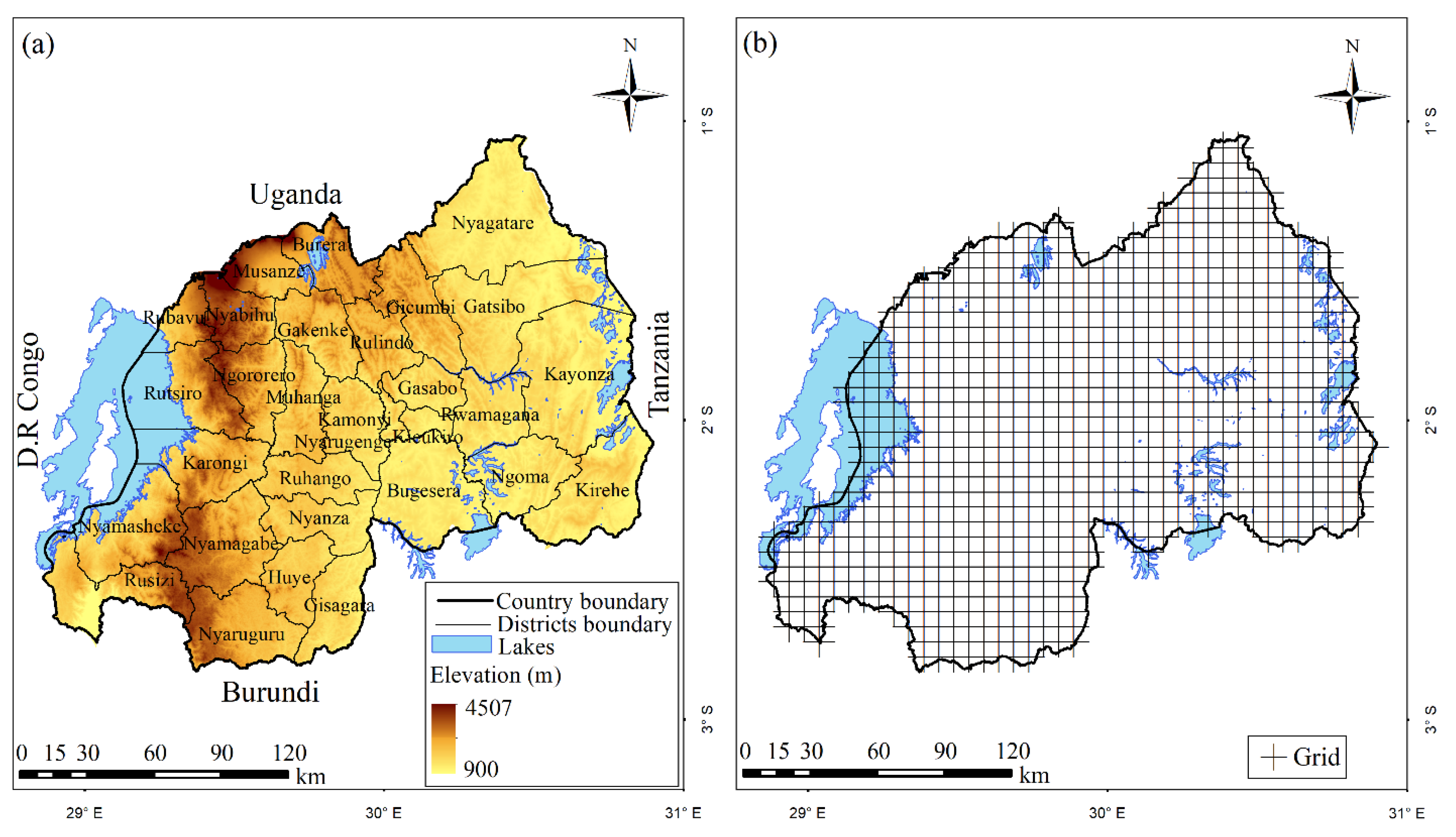
2.1. Study Area

Rwanda is part of the East Africa region with total area of 26,338 km², where land area is about 24,950 km² (94.7%), and inland lakes cover about 1390 km² (5.3%) (Figure 1a). Agricultural land covers 14,020 km² (59%) of total country land. The hydrological network comprise numerous lakes, rivers, and associated wetlands. The topography of Rwanda is complex, ranging from high to lowland areas, with a mixture of mountains, hills, and valleys. Rwanda has five climate types [59]: The first is the savanna type located in the East-Rwandan dry and hot lowland zone lying from the border with neighboring Tanzania in the east and stretching gradually from east to west and spreading beyond the surrounding area of the capital, Kigali City. The second is the temperate type located in the central highlands zone with elevation that increases from east to west. In that area, rainfall also increases markedly following the elevation. The third is the humid mountain climate type covering southern Rwanda area, especially around the Nyungwe National Park located on the Congo-Nile Divide. The fourth is the dry mountain climate type found in the Virunga National Park, located in the volcanic mountains of northern region. The fifth is Kivu-sea climate type along the coastal ridge of Lake Kivu, where land–lake–wind circulation interacts with high evaporation rates prevailing on Lake Kivu to create amounts of rainfall on the western bridge of the Congo-Nile watershed, thus making it a distinct regional climate system.

The country experiences four seasons: the short dry season (January–February, JF), the long rain season (March–April–May, MAM), the long dry season (June–July–August, JJA), and the short rain season (September–October–November–December, SOND). In general, maximum and minimum temperatures decrease gradually with topography from the eastern to the western parts of the country in all seasons. The average temperature for Rwanda is around 20 °C and varies with the topography. The warmest annual average temperatures are found in the eastern plateau (20–21 °C) and south-eastern valley of Rusizi (23–24 °C) in the south-west, and cooler temperatures are found in higher elevations of the central plateau (17.5–19 °C) and high-lands (<17 °C) in the north and north-west.

According to Fifth National Population and Housing Census held in 2022 [60], the country’s population is 13,246,394, which corresponds to an annual growth rate of 2.3% between 2012 and 2022. Men represent 48.5% of the population, while women represent 51.5%. The population accessing improved drinking water is 79%, while 12% have access to safely managed water drinking services. In total, 72.1% of Rwandans live in rural areas, while 27.9% live in urban areas. In 2022, GDP at current market prices was estimated at RWF 13,716 billion. Services sector contributed 47% of GDP, agriculture sector contributed 25% of the GDP, and industry sector contributed 21% of GDP, while 7% was attributed to adjustment for taxes and fewer subsidies on products.

Despite the recent experience that the East African region has known and knows today, the impacts of climate change have not spared Rwanda [14,15,16]. The country has committed to undertake adaptation and mitigation measures to the greatest extent possible for vulnerable communities. However, to achieve this, it is necessary to have objective information from scientifically analyzed meteorological observations. With the development that Rwanda has experienced during last decades after 1994 Genocide Against the Tutsi, meteorological services have significantly increased their capacity and the number of active meteorological stations covering the whole country. This enabled us to undertake an initiative, via collaboration with experts, of displaying observed meteorological data on a grid of 5 km resolution [61,62]. The resulting gridded data set consisted of a combination of quality controlled station data with satellite data for rainfall and reanalysis data for temperature to fill the gaps. Such development has motivated researchers to undertake some studies on climate change in Rwanda.

2.2. Data and Methods

2.2.1. Data

Gridded data sets of the maximum and minimum temperatures covering the period from 1983 to 2022 at a spatial resolution of 0.05 degrees (~5 km) were provided by the Rwanda Meteorology Agency (Meteo Rwanda). They can be accessed online at https://www.meteorwanda.gov.rw, accessed on 1 August 2023. They were reconstructed in Meteo Rwanda following the methodology described by Dinku et al. [61] and Siebert et al. [62]. A quality control (homogeneity test, missing data, and outliers) was first carried out on temperature data from 66 Rwandan weather stations. To address temporal and spatial gaps in the data time series, a combination with bias-adjusted Japanese 55-year reanalysis project (JRA55) was then performed.

2.2.2. Methods

Extreme Temperature Indices

Five extreme temperature indices (

Table 1. List of extreme temperature indices used in this study.

Index	Description	Definition	Unit	Reference
DTR	Diurnal temperature range	Annual mean difference between daily maximum and minimum temperature	°C	Folland et al. [67]
Tn10p	Cold nights	Number of days in a year with minimum temperature below a threshold corresponding to 10th percentile of daily minimum temperature distribution in the 1991–2020 baseline period.	days/year	Karl et al. [63] Zhang et.al [64] Tank et al. [65]
Tx10p	Cold days	Number of days in a year with maximum temperature below a threshold corresponding to 10th percentile of daily maximum temperature distribution in the 1991–2020 baseline period.	days/year	Karl et al. [63] Zhang et.al [64] Tank et al. [65]
Tn90p	Warm nights	Number of days in a year with minimum temperature above a threshold corresponding to 90th percentile of daily minimum temperature distribution in the 1991–2020 baseline period.	days/year	Karl et al. [63] Zhang et.al [64] Tank et al. [65]
Tx90p	Warm days	Number of days in a year with maximum temperature above a threshold corresponding to 90th percentile of daily maximum temperature distribution in the 1991–2020 baseline period.	days/year	Karl et al. [63] Zhang et.al [64] Tank et al. [65]

) were computed based on the methodology provided by Expert Team on Climate Change Detection and Indices (ETCCDI) [63,64,65]. Percentile-based threshold indices were computed for each calendar day using data for consecutive 5-day moving windows centered on that calendar day [65] from the 1991–2020 base period. The computation of extreme temperature indices and their corresponding thresholds was carried out using RClimDex v1.0 base package [66].

The Mann–Kendall (MK) Trend Test and Theil–Sen’s Slope Estimator (TSS)

The non-parametric Mann–Kendall test and the Theil–Sen’s slope estimator approach are widely used as trend tests as well as for estimation of magnitudes of trends in hydrology and climate time series [23,68,69]. They have been recommended by the World Meteorological Organization (WMO) owing to their compatibility with non-normalized data as well as missing values [68].

▪

The Mann–Kendall test

Let $\left(x_1,y_1\right), \left(x_2,y_2\right), \dots , (x_n,y_n)$ be a set of joint observations from two random variables $X$ and $Y$ respectively, such that all the values of the couple $(x_i,y_i)$ are unique. Kendall’s rank correlation measures the strength of monotonic association between the vectors $X$ and $Y$.

The Mann–Kendall test statistic is calculated from the sum of the signs (+ or −) of the slopes. The statistic S called Kendall score is expressed as

$$S=\sum _{k=1}^{n-1}\sum _{j=k+1}^{n}sign(x_j-x_k)$$

(1)

where $n$ is the length of the sample, $x_k$ and $x_j$ are from $k=1, 2, \dots , n-1$ and $j=k+1, 2, \dots , n,$ and the $sign\left(x_j-x_k\right)$ is an indicator function that takes on the values 1, 0, or −1, as indicated below:

$$sign\left(x_j-x_k\right)=\left\{\begin{array}{c}+1 if \left(x_j-x_k\right)>0\\ 0 if \left(x_j-x_k\right)=0\\ -1 if \left(x_j-x_k\right)<0\end{array}\right.$$

(2)

If $n\ge 10$, the statistic $S$ is approximately normally distributed with the mean $\left(S\right)=0$, and the variance of $S$ can be obtained as follows:

$$var\left(S\right)=\frac{n\left(n-1\right)\left(2n+5\right)-\sum _{j=1}^p{t}_j(t_j-1\left)\right(2t_j+5)}{18}$$

(3)

where $p$ is the number of ties in the series, and $t_j$ is the number of data points in the jth tied group.

For trend test, the variable $Y$ can be time. The presence of statistically significant trend is evaluated using the $Z$ value. This statistic is used to test the null hypothesis such that no trend exists. The standardized test statistic Z is given via

$$Z=\left\{\begin{array}{c}\frac{S-1}{\sqrt{var\left(S\right)}}, if S>0\\ 0, if S=0\\ \frac{S+1}{\sqrt{var\left(S\right)}}, if S<0\end{array}\right.$$

(4)

The trend is said to be increasing (decreasing) if $Z$ is positive (negative). To test for either increasing or decreasing monotonic trends with confidence level α, the null hypothesis $H_0$ is rejected if $\left|Z\right|>Z_{(1-\alpha /2)}$, where $Z_{(1-\alpha /2)}$ is the corresponding value of $p=\alpha /2$, following the standard normal cumulative distribution tables, and represents the standard normal deviates, and $p$ is the significant level for the test.

▪

Autocorrelation

The presence of positive or negative autocorrelation in the time series may increase the possibility of detecting trends while there is no trend and vice versa [70,71,72,73]. The existence of positive autocorrelation in the series can lead the Mann–Kendall test to a conclusion of the presence of trend in the series, while it may not be always true. On the other hand, the existence of negative autocorrelation in the series can lead to the opposite.

The coefficient of autocorrelation ${\rho }_k$ of a discrete time series for lag-k is obtained following the formula adopted by Datta and Das [74] as follows:

$${\rho }_k=\frac{\sum _{i=1}^{n-k}(x_i-\overline{x})(x_{i+k}-{\overline{x}}_{i+k})}{{⌊\sum _{i=1}^{n-k}{(x_i-\overline{x})}^2\times \sum _{i=1}^{n-k}{(x_{i+k}-{\overline{x}}_{i+k})}^2⌋}^{\frac{1}{2}}}$$

(5)

▪

The Modified Mann–Kendall (MMK) test

A modified Mann–Kendall test was proposed by Ahmed et al. [75] to take into consideration the influence of autocorrelation in data, which is often ignored. A correction is brought to the variance of $S$ [70,76,77,78], which is replaced by

$${var}^{*}\left(S\right)=var(S)\frac{n}{n_k^{*}}$$

(6)

where $\frac{n}{n_k^{*}}$ represents a correction due to the autocorrelation in the data and is given via

$$\frac{n}{n_k^{*}}=1+\frac{2}{n(n-1)(n-2)}\sum _{i=1}^{n-1}(n-i)(n-i-1)(n-i-2){\rho }_k$$

(7)

where $n$ is the actual number of observations, $n_k^{*}$ represents the effective number of observations to account for the autocorrelation in the data, and ${\rho }_k$ is the autocorrelation function of the ranks of the observations. As the non-significant values of ${\rho }_k$ can badly affect the precision of the variance of $S$, and thus, only significant ${\rho }_k$ values are opted to estimate $\frac{n}{n_k}$ [79]. In this method, the autocorrelation $s {\rho }_k$ between ranks of the observations have been calculated from the respective time series after subtracting from the time series an estimate of Sen’s slope (described below) from the data. The Mann–Kendall test was then applied with the corrected variance ${var}^{*}\left(S\right)$.

▪

Theil–Sen slope estimator

In a case where a linear trend exists in a time series, the slope or magnitude of that trend can be detected using a simple non-parametric procedure first developed by Theil [80] and later modified by Sen [81]. Sen’s slope has the advantage over the slope of regression, in the sense that gross data series errors and outliers do not affect it much. The slope is determined to be the mean of all pair-wise slopes for any pair of points in the dataset. The following equation is used to estimate each individual slope:

$$Q_{ij}=\frac{x_j-x_i}{j-i}, j>i, \mathrm{for} i=\mathrm{1,2},\dots ,N$$

(8)

If in the time series, there are $n$ values of $Q_{ij}$, estimates of the slope will be $N=n(n-2)/2$. The slope of the Sen Estimator is the mean slope of such $N$ values of pair-wise slopes. The Sen’s slope is obtained using

$$Q=\mathrm{Median}\left(\frac{x_j-x_i}{j-i}\right), j>i, \mathrm{for} i=\mathrm{1,2},\dots ,N$$

(9)

$$Q=\left\{\begin{array}{c}{Q}_{⌈\frac{N+1}{2}⌉} if n is odd\\ \frac{1}{2}\left(Q_{\frac{N}{2}}+Q_{⌊\frac{N+2}{2}⌋}\right) if n is even\end{array}\right.$$

(10)

Positive value of $Q$ indicates an upward or increasing trend and a negative value of $Q$ gives a downward or decreasing trend in the time series.

In this present study, trends were computed at each grid point for time series of maximum temperature, minimum temperature, and extreme temperature indices using the Modified Mann–Kendall non-parametric rank statistic test [82] and the Theil–Sen (TS) estimator approach [83] for, respectively, trend analysis and slope estimation. Trends were computed at the scale of a year and then converted at a scale of decade for analysis. Significant trends were considered at confidence level α = 0.05. The standard deviation was computed at each grid for time series of respective indexes to represent their variabilities. They were computed and then analyzed at annual scale for the period of study. In climate studies, spatial interpolation is important for local analysis by Geographic Information Systems (GIS). Two different methods are commonly used: the Kriging method and Inverse Distance Weighted (IDW) method [84,85]. Kriging method is a geostatistical interpolation method that takes into consideration the distance and the degree of variation between known data points when estimating values at neighboring unknown locations. IDW uses a linear weighted combination of known data points, taking into account the distance, i.e., giving more weight to a closer data point and less weight to distant one. The advantage of Kriging interpolation method to IWD is that it is statistically optimal interpolator for dense and well spatially distributed data [86]. However, IWD interpolation method may be preferred over Kriging for sparse data. In this present study, maps were generated using Kriging interpolation method for spatial interpolation with the ArcGIS10 software. Spatially aggregated mean maximum temperature, minimum temperature, and extreme temperature indices were computed by taking simple arithmetic averages of respective indexes for all grids, and their trends were further analyzed.

3. Results

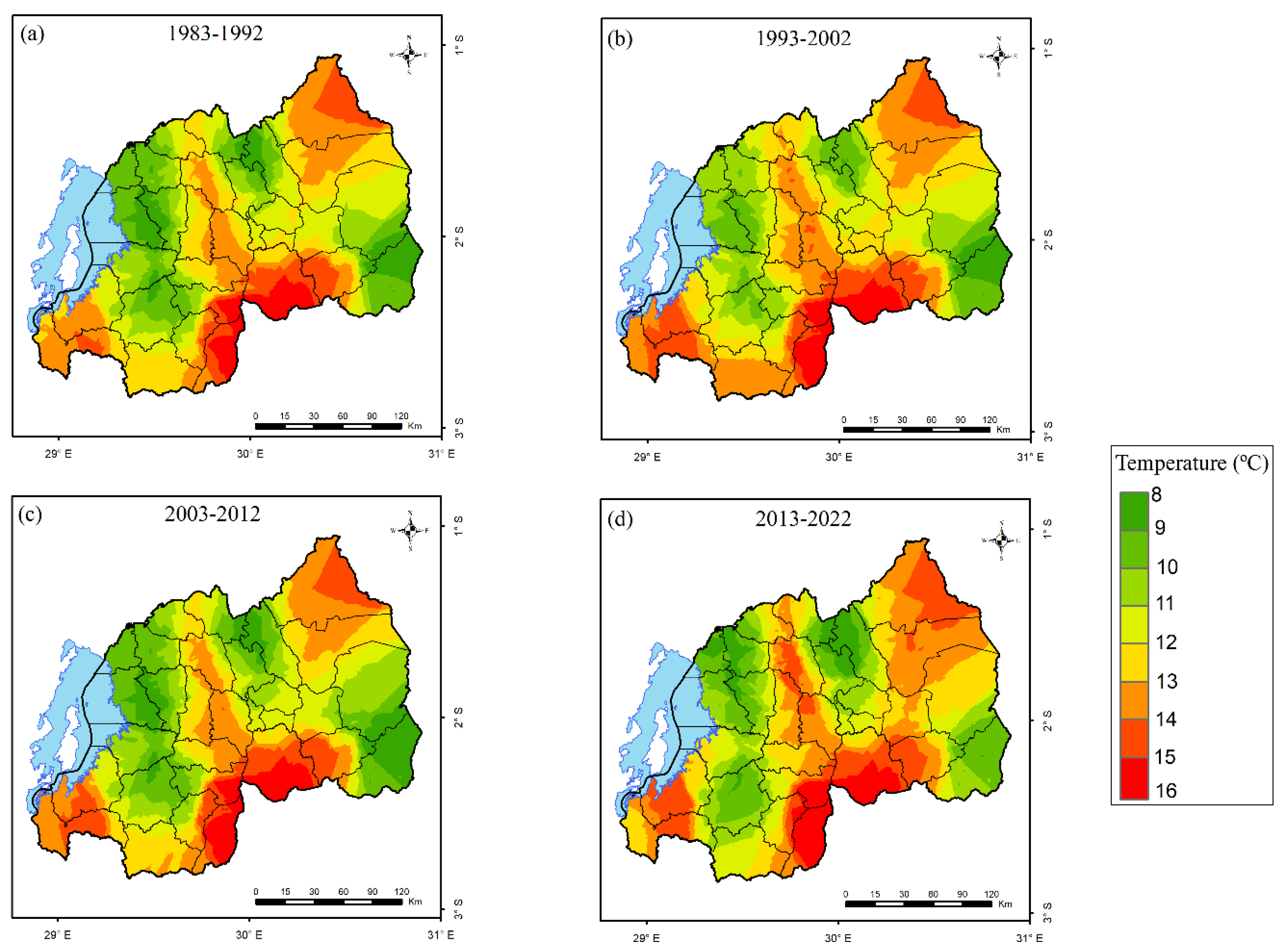
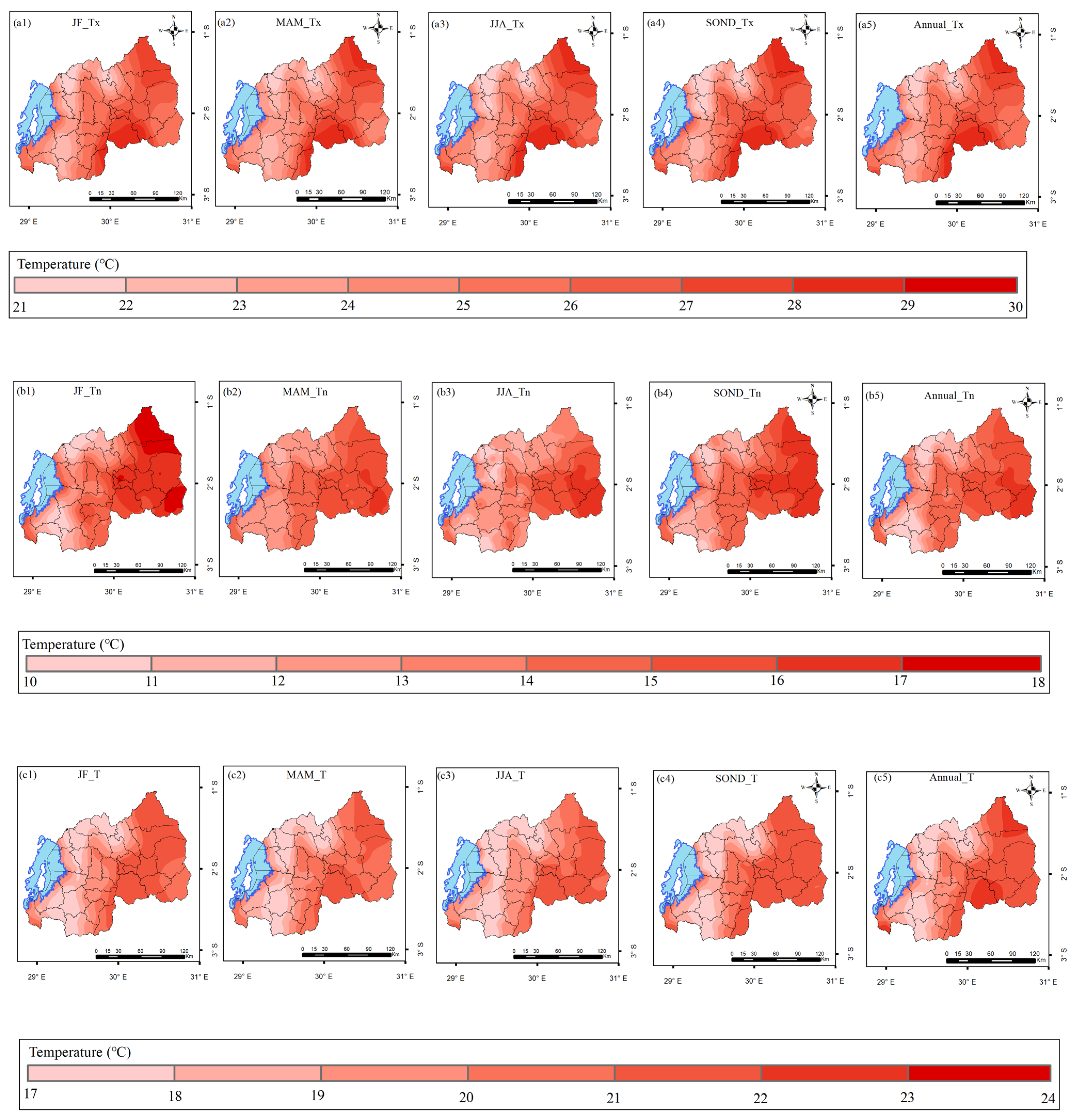
3.1. Spatial Distributions of Long-Term Mean of Tx, Tn, and T

Figure 2 presents the spatial distribution of the long-term mean of Tx, Tn, and T over Rwanda during the period of 1983–2022. In general, Tx, Tn, and T decrease gradually with topography from the eastern to the western parts of the country in all seasons. Tx and T have maximum values during the JJA and JF seasons and minimum values during MAM and SOND. Tn has the lowest value during JJA and the highest value during MAM.

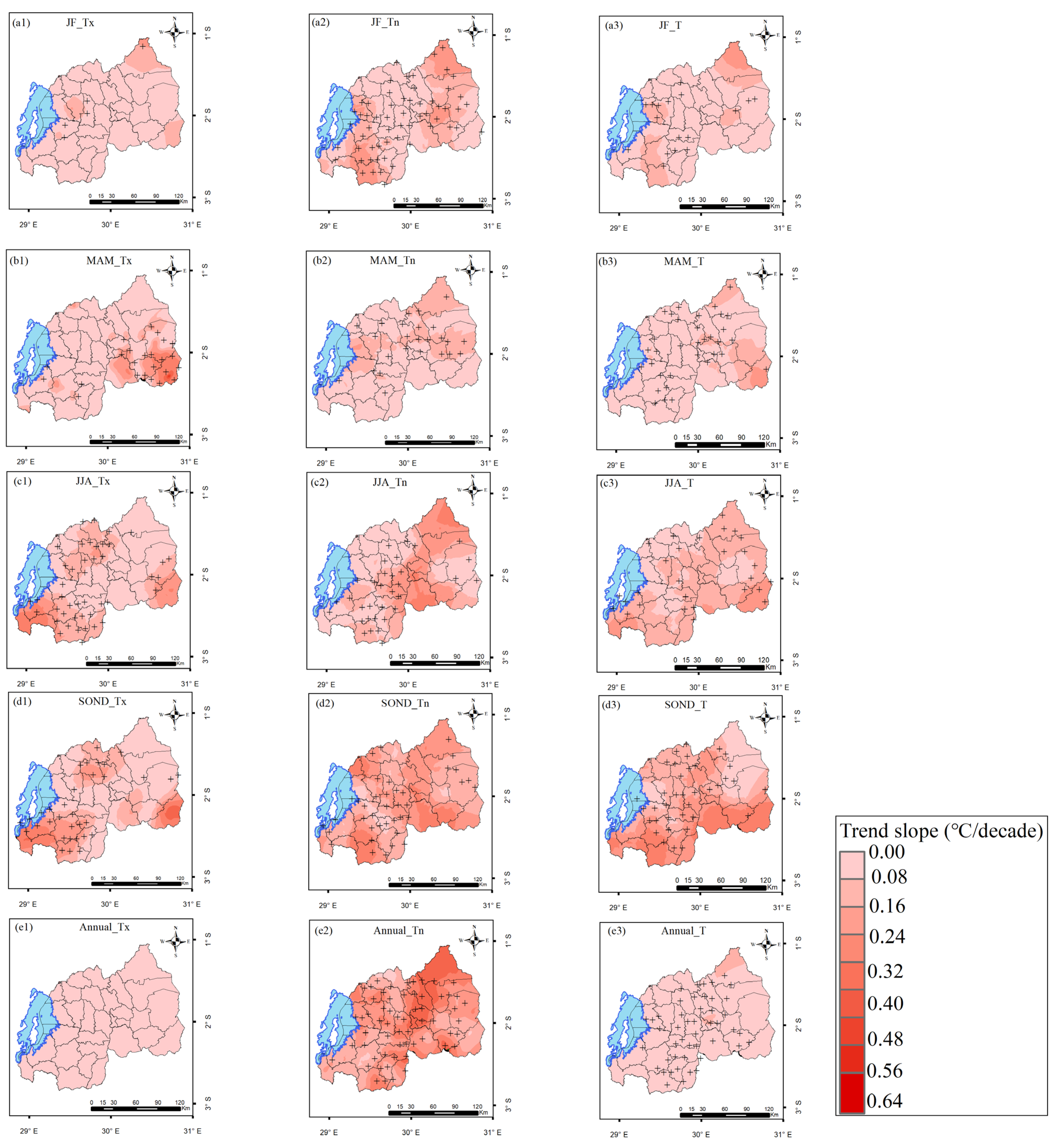
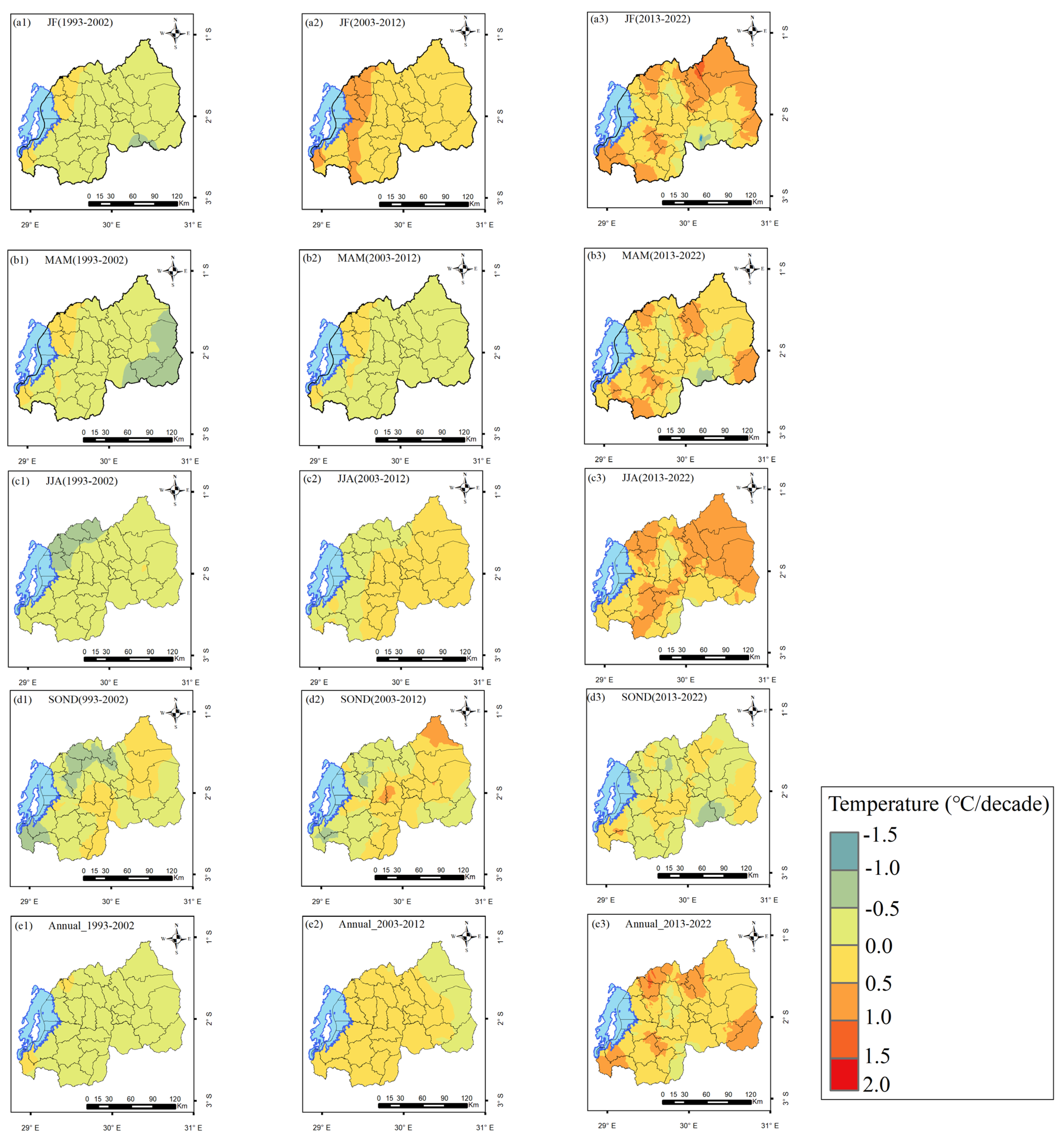
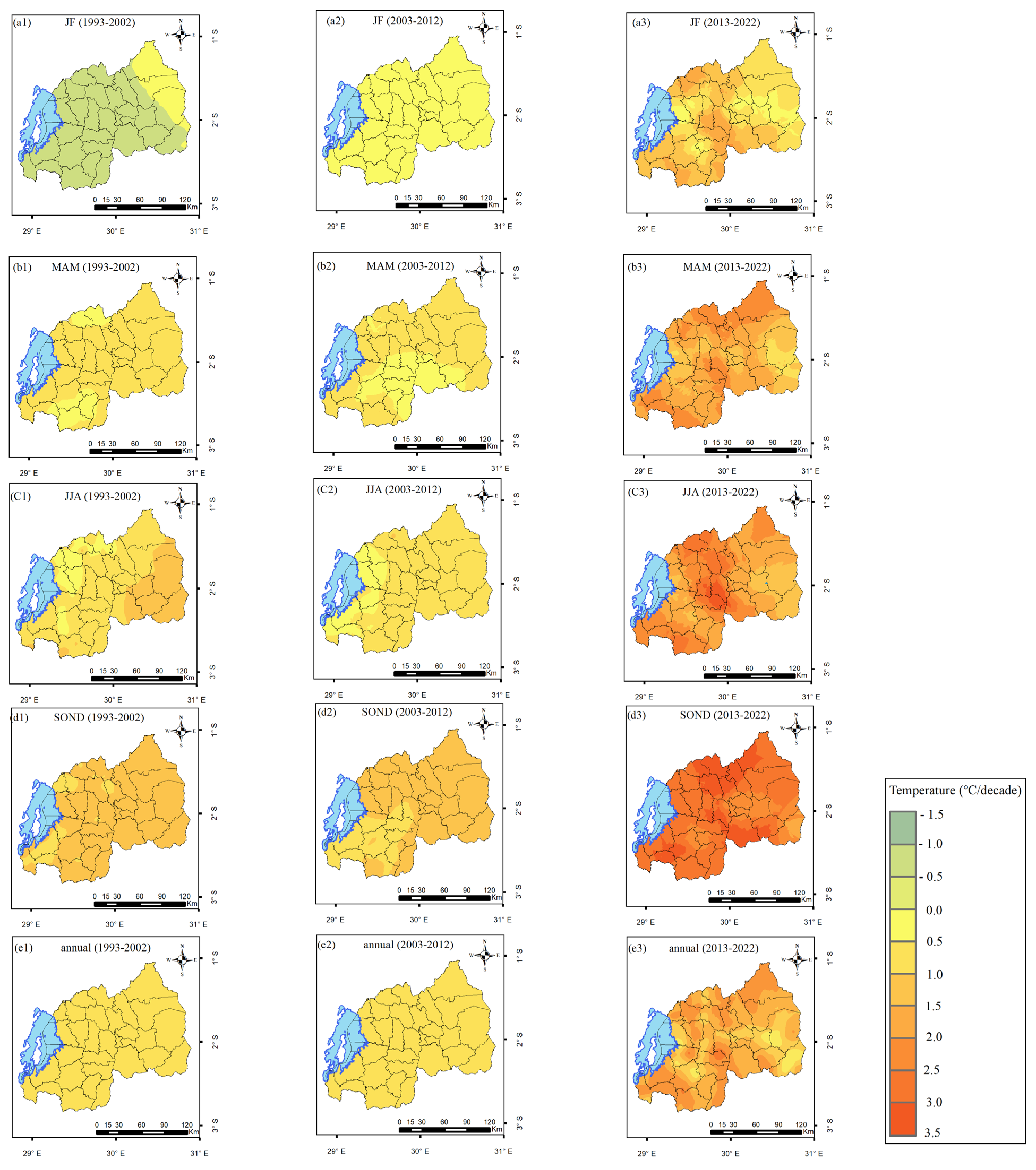
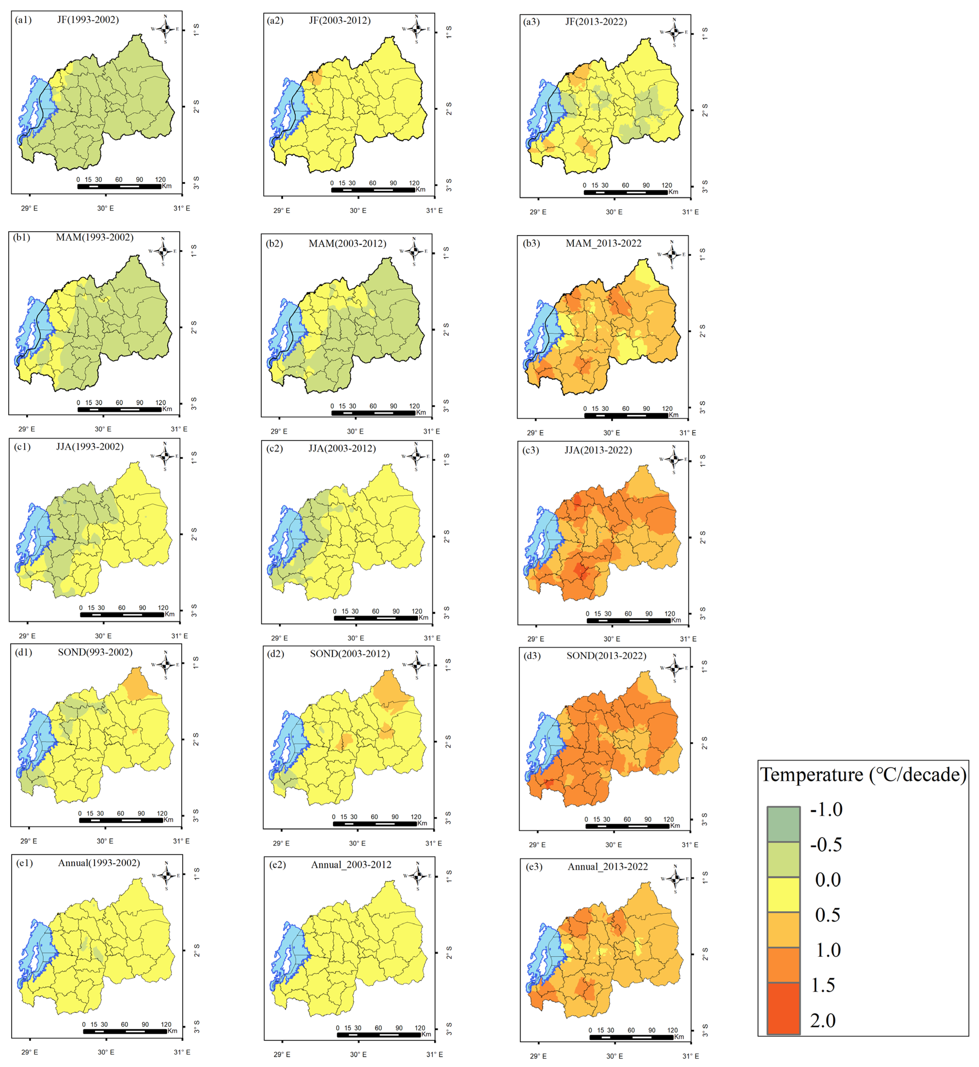
3.2. Trends of Temperatures

Figure 3 presents the spatial distribution of trends Tx, Tn, and T over Rwanda during the period of 1983–2022 expressed in °C/decade for seasons and the annual average. In general, temperatures decrease gradually with topography from the eastern to the western parts of the country in all seasons. The analysis of the spatial distribution of the trends of temperatures indicates that for Tx, the southeastern (Kirehe District) and the southwestern (Nyamasheke and Rusizi Districts) present the highest but moderate statistically significant positive trend (0.24–0.40 °C/decade) during JJA and SOND. During MAM, the southeastern part of the country (Kirehe District) indicates statistically significant high positive trends (0.40–0.56 °C/decade). For Tn, statistically high significant positive trends (0.48–0.64 °C/decade) are observed during SOND across the country. No statistically significant trend is observed for the annual mean of Tn. As for T, statistically significant high positive trends (0.24–0.40 °C/decade) are observed over the southeastern part of the country (Kirehe District) during MAM and over the southwestern (Nyamasheke and Rusizi Districts) and southern of the eastern region (Bugesera and Ngoma Districts) during SOND. Statistically significant increasing trends are observed for spatially averaged Tn during JJA (0.17 °C/decade) and SOND (0.20 °C/decade) as well for T during SOND (0.16 °C/decade).

Table 2. Trends of spatially averaged Tx, Tn, and T during JF, MAM, JJA, SOND, and mean annual over Rwanda during the period of 1983–2022 expressed in °C/decade.

Tn
Season	Z	Tau	Sen’s Slope	p-Value	Significance
JF	0.456	0.051	0.000	0.648	No
MAM	0.949	0.105	0.007	0.342	No
JJA	2.444	0.269	0.017	0.015	Yes
SOND	2.538	0.279	0.020	0.011	Yes
ANNUAL	2.063	0.227	0.013	0.039	Yes
Tx
Season	Z	tau	Sen’s Slope	p-value	Significance
JF	−1.133	−0.126	−0.010	0.257	No
MAM	1.358	0.150	0.013	0.174	No
JJA	−1.535	−0.169	−0.010	0.125	No
SOND	1.367	1.367	0.010	0.172	No
ANNUAL	0.188	0.022	0.000	0.851	No
T
Season	Z	tau	Sen’s Slope	p−value	Significance
JF	−0.281	−0.032	0.000	0.779	No
MAM	1.217	0.135	0.008	0.224	No
JJA	1.280	0.141	0.005	0.201	No
SOND	2.839	0.312	0.016	0.005	Yes
ANNUAL	1.708	0.187	0.007	0.088	No

presents the trends of spatially averaged Tx, Tn, and T for JF, MAM, JJA, SOND, and mean annual during the period of 1983–2022. Statistically significant increasing trends are observed for spatially averaged Tn during JJA (0.17 °C/decade) and SOND (0.20 °C/decade) as well for T during SOND (0.16 °C/decade).

Figure 4 indicates the decadal differences in Tx for JF, MAM, JJA, SOND, and annual mean with reference to the period of 1983–1992.

Figure 5 indicates the decadal differences of Tn for JF, MAM, JJA, SOND, and annual mean with reference to the period of 1983–1992. During the second decade (1993–2002), the JF season shows a general reduction in Tn countrywide. The northeastern part shows a lower decrease (−0.5–0.0 °C) compared to the remaining parts of the country (−1.0–−0.5 °C). Increases in Tn (0.0–1.0 °C) are seen in many areas during MAM, JJA, and the year. During SOND, increases in Tn (1.0–1.5 °C) are observed in most parts of the country. The same range of increase is observed over the eastern part during the JJA season. During the third decade (2003–2012), relatively low increases in Tn (0.0–0.5 °C) are observed countrywide during JF season. During MAM, increases in Tn (0.5–1.0 °C) are observed in many parts of the country, while low increases ([0.0, 0.5] °C) are observed in the southeastern part. During JJA, increases in Tn (0.5–1.0 °C) are observed in many parts of the country, while low increases (0.0–0.5 °C) are observed in the western areas. During the SOND season, most parts of the country experienced increases in Tn (1.0–1.5 °C), while an increase of 0.5–1.0 °C was observed over the southwestern region. Annually, increases in Tn (0.5–1.0 °C) are found in all parts of the country. During the fourth decade (2013–2022), increases in Tn (0.5–1.0 °C) were observed over the central eastern and central western parts, while increases in Tn ([0.1, 1.5] °C) were observed over the remaining parts of the country. During MAM, increases in Tn (0.5–1.0 °C) are observed over the central eastern part, while there were increases in Tn (1.5–2.0 °C) in the remaining parts of the country. During JJA, it is observed that increases in Tn (2.5–3.0 °C) in the central plateau extend to the western highland, while increases in Tn (2.0–2.5 °C) are observed in the remaining parts of the country. During SOND, increases in Tn (3.0–3.5 °C) are observed countrywide. On an annual basis, increases in Tn (0.5–1.0 °C) are observed over the central eastern and central western parts, while increases in Tn (1.0–1.5 °C) are observed in the remaining parts of the country.

Figure 6 indicates the decadal differences in T for JF, MAM, JJA, SOND, and annual mean with reference to the period of 1983–1992.

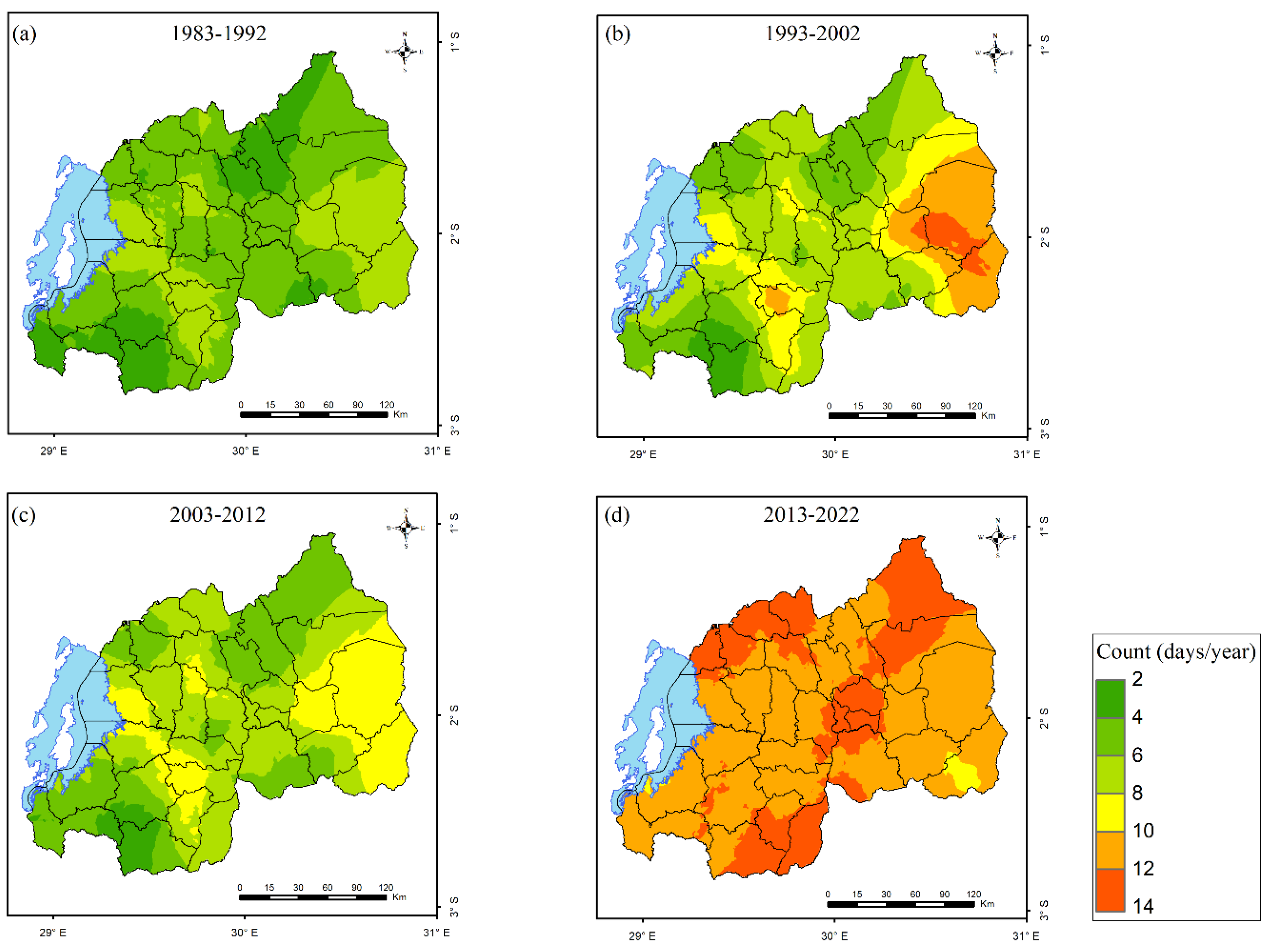
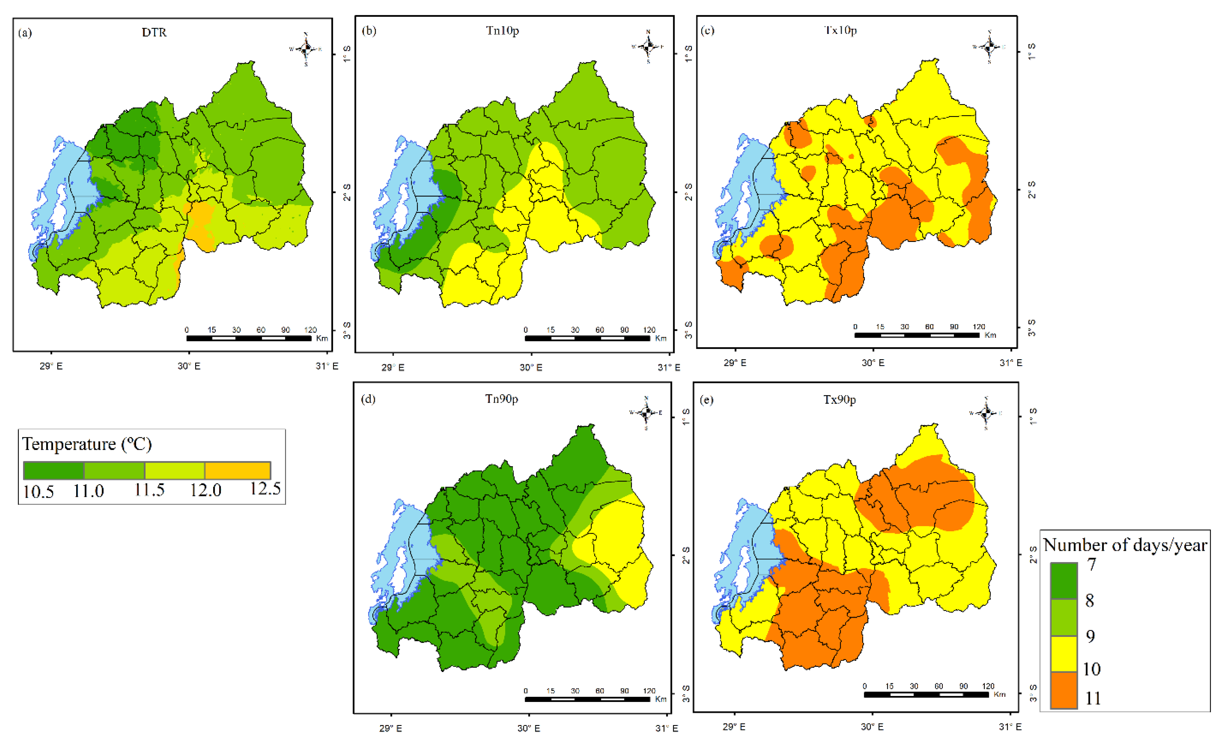
3.3. Spatial Distributions of Long-Term Mean of DTR, Tn10p, Tx10p, and Tn90p

Figure 7 indicates the spatial distribution of the long-term mean of DTR, Tn10p, Tx10p, Tn90p, and Tx90p over Rwanda for the period of 1983–2022. For DTR (Figure 7a), four distinguished parts are observed: the northwestern region (10.5–11 °C), the part extending from the south to the southeastern region (11.5–12.0 °C), the south-central parts of the country (12.0–12.5 °C), and the remaining parts of the country (11.0–11.5 °C). For Tn10p (Figure 7b), three distinguished parts are observed: the extreme western region ([7,8] days/year), the part extending from the south to central parts (9–10 days/year), and the remaining parts of the country (8–9 days/year). For Tx10p (Figure 7c), two distinguished parts are observed: the south, central, and extreme eastern parts (10–11 days/year) and the remaining parts of the country (9–10 days/year). For Tn90p (Figure 7d), two distinguished parts are observed: the central eastern and southeastern (9–10 days/year) and the remaining parts of the country (7–8 days/year). For Tx90p (Figure 7e), two distinguished parts are observed: the southern and northeastern (10–11 days/year) and the remaining parts of the country (9–10 days/year).

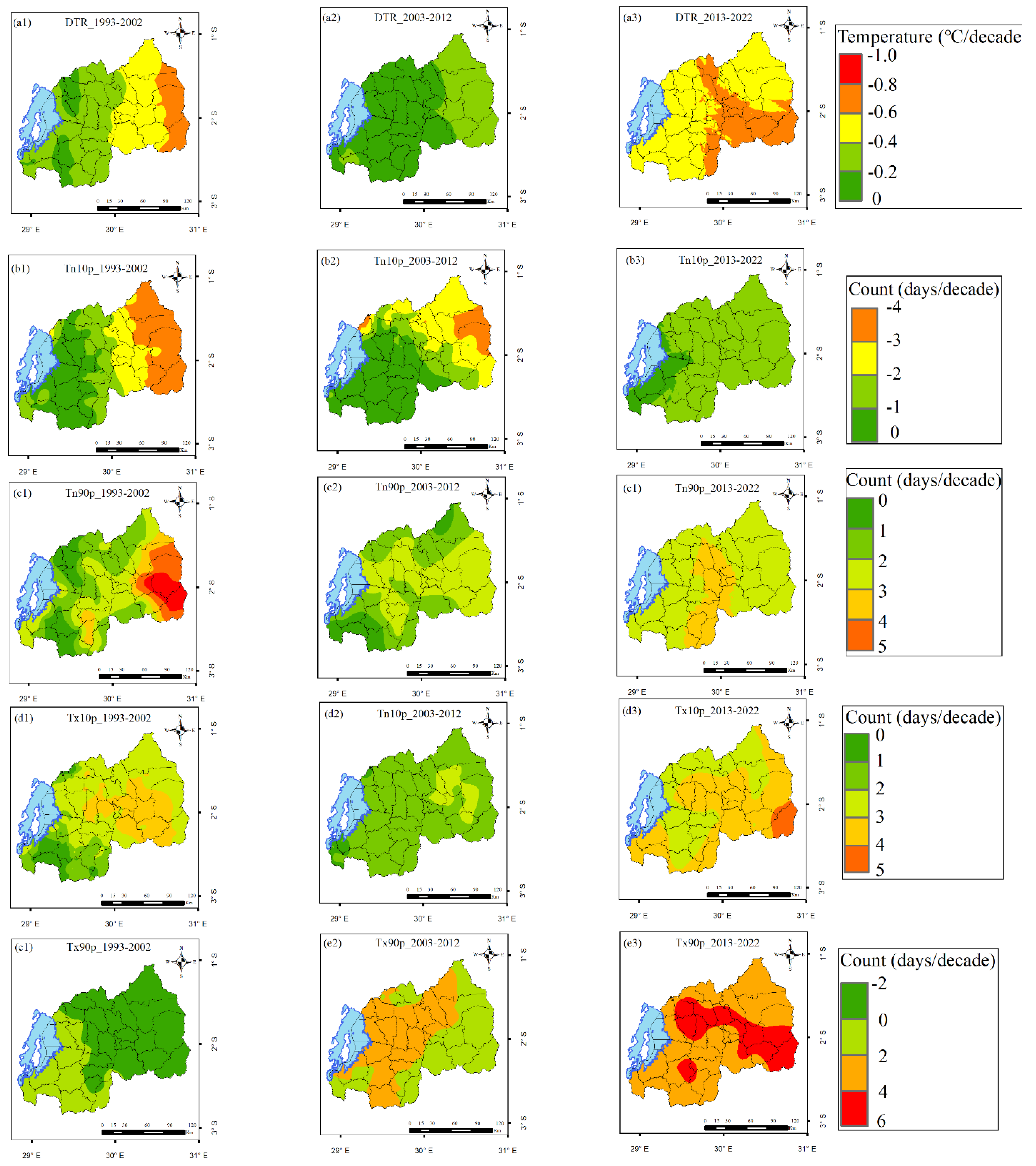
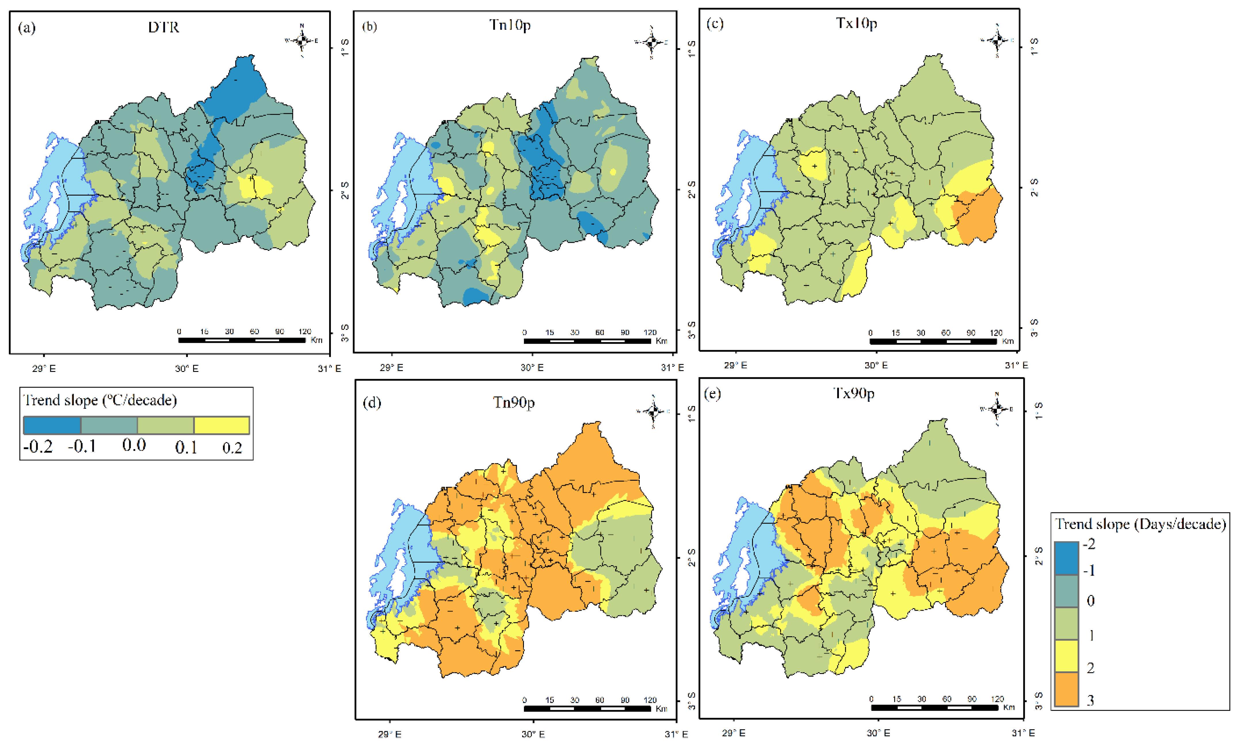
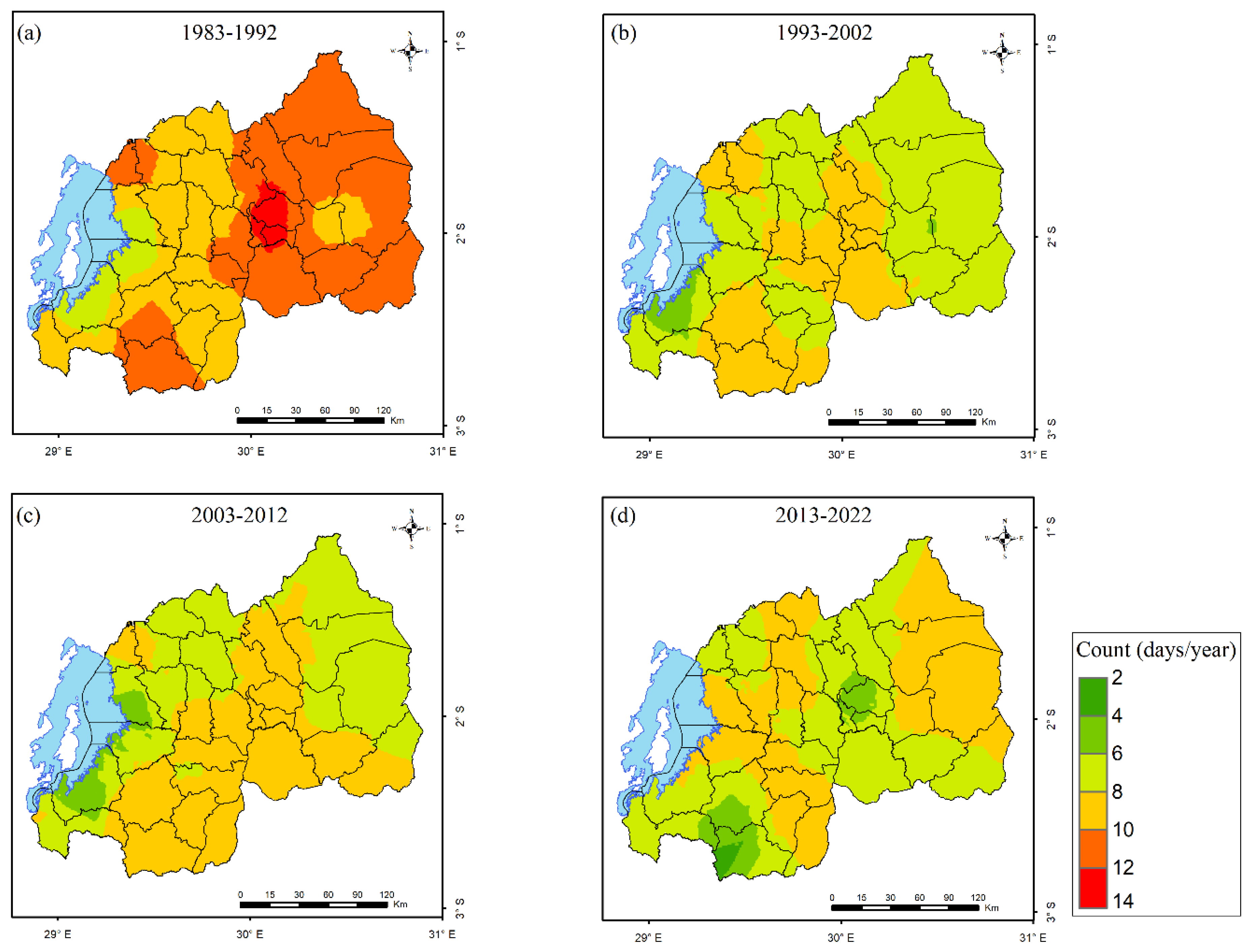
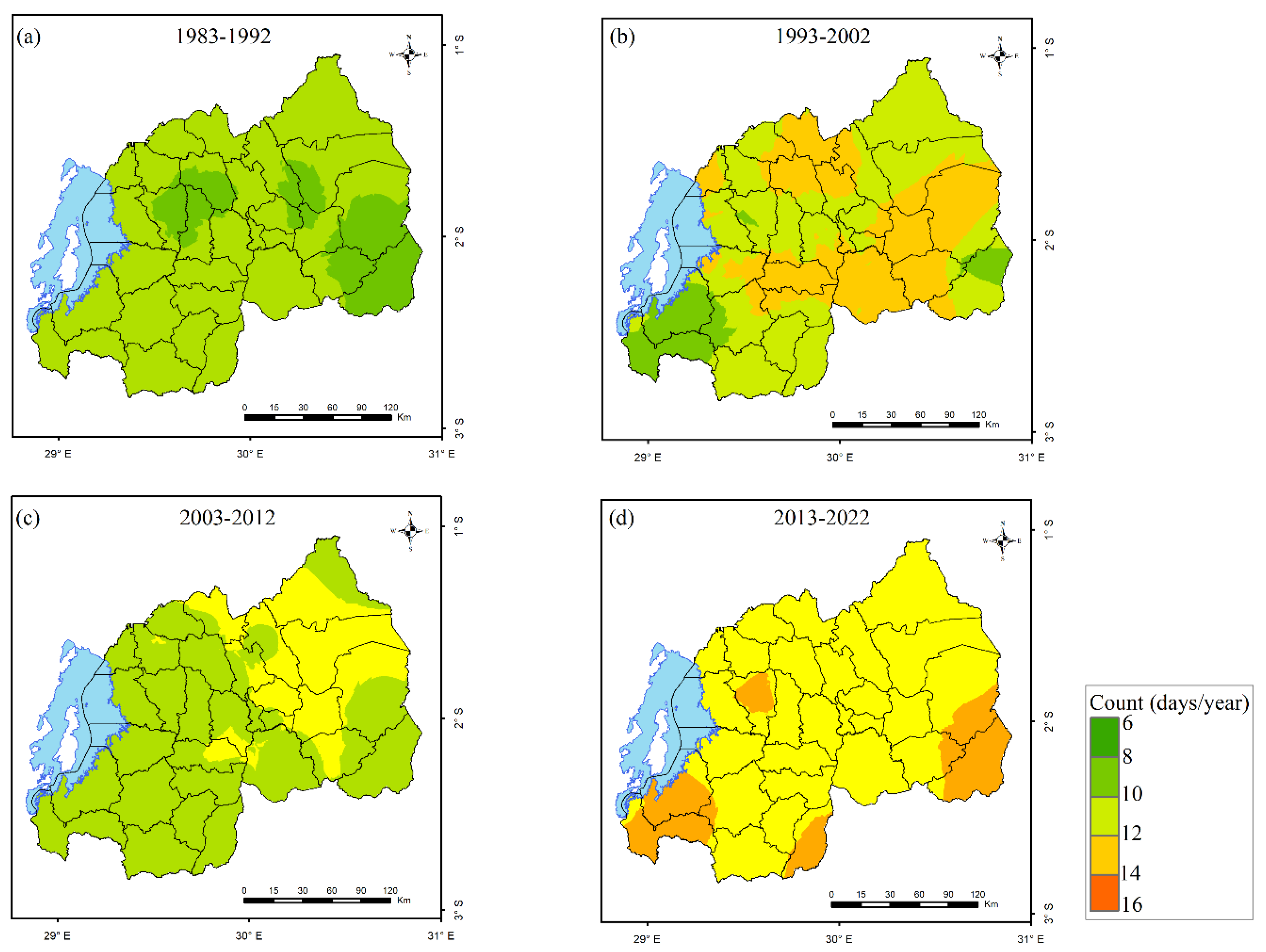
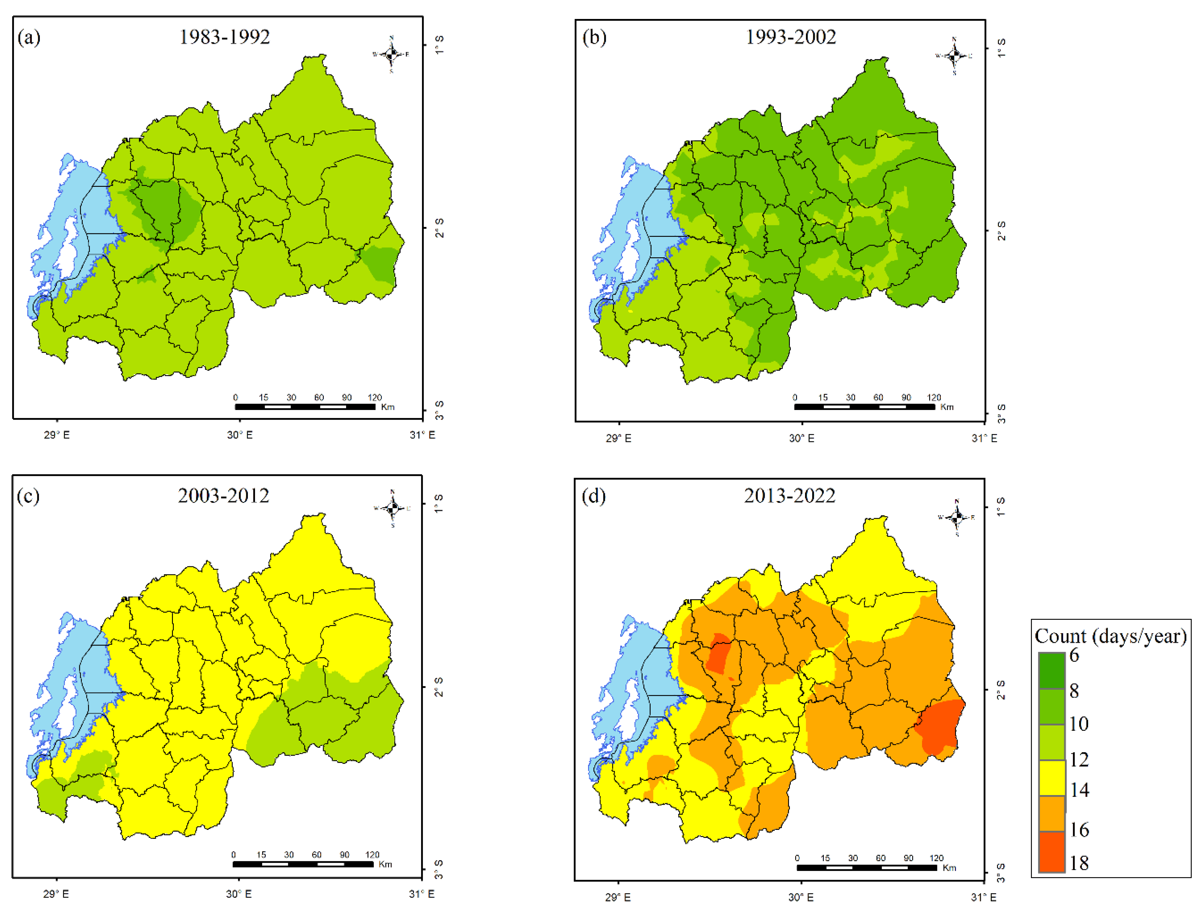
3.4. Trends of Extreme Indices

Figure 8 indicates the spatial distribution of trends of DTR, Tn10p, Tx10p, Tn90p, and Tx90p. Overall, a statistically significant decrease in DTR is observed in most parts of the country except the eastern region and small parts of the western region. The central part (Kigali City and Gicumbi Districts) extended to the northeastern part of the country (Nyagatare District) and exhibits the highest decrease (−0.2–0.0 °C/decade) of DTR. Tn10p presents statistically significant negative trends over the whole country except in a narrow band along the Congo-Nile Divide. The central part of the country (Kigali City, Rulindo, and Gicumbi Districts) has the highest decrease (−2–0 days/decade) of Tn10p. Tn90p presents statistically significant positive trends in most parts of the country. The central part (Kigali City, Kamonyi, Ruhango, Bugesera, and Gicumbi District) extended to the northeastern part (Nyagatare and Gatsibo District), the southern part (Huye, Nyaruguru and Nyamagabe Districts), and the northwestern part of the country (Rubavu, Nyabihu, Musanze and Burera Districts), which presented a high increase (2–3 days/decade) in Tn90p. Tx10p exhibits positive trends over the whole country. Statistically significant high positive trends (1–3 days/decade) are observed on one side in the south-central eastern (Gisagara, Nyanza, and Bugesera Districts) and central eastern parts (Rwamagana District) and on the other side in some portions of the southeastern parts of the country (Kirehe, Kayonza, and Ngoma Districts). Tx90p exhibits over the whole country positive trends. Statistically significant high positive trends (2–3 days/decade) are observed in the western highland (Muhanga, Ngororero, Rutsiro, Rubavu, Nyabihu Musanze, and Gakenke Districts) and central parts of the eastern region (Rwamagana, Ngoma, Kayonza and Kirehe Districts).

Table 3. Trends of spatially averaged DTR_(a) (°C/year) and Tn10p_(b); Tx10p_(c); Tn90p_(d); and Tx90p_(e) (days/year) over Rwanda during the period of 1983–2022.

Season	Z	Tau	Sen’s Slope	p-Value	Significance
DTR	−2.307	0.255	−0.014	0.021	Yes
Tn10p	−0.851	0.095	−0.049	0.395	No
Tn90p	1.317	0.146	0.062	0.029	Yes
Tx10p	2.342	0.259	0.084	0.019	Yes
Tx90p	2.552	0.282	0.128	0.011	Yes

presents the spatially averaged trends of DTR, Tn10p, Tx10p, Tn90p, and Tx90p. Spatially averaged DTR shows a statistically significant decreasing trend (−0.14 °C/decade), while spatially averaged Tn90p, Tx10p and Tx9p show statistically significant increase trends (0.62, 0.84, and 1.28 days/decade).

Figure 9 indicates the DTR for various decades of this present study. Overall, the first three decades (Figure 9a–c) show high values compared to the fourth decade (Figure 9d). The western region, the southeastern region, and small parts of the northern region show low values of DTR (8–10 °C) for all decades. The south-central eastern and northeastern parts indicate high values of DTR (13–16 °C). The remaining parts of the country present moderate values of DTR (10–13 °C).

Figure 10 presents Tn10p for various decades of this present study. During the first decade (Figure 10a), high values (12–14 days/year) are observed in the central region. The southwestern, northwestern highlands, central plateau, and eastern region indicate relatively high values (10–12 days/year). Moderate values (8–10 days/year) are observed over the central and western highlands, while the remaining parts of the country experienced low values (4–6 days/year). During the second and third decades (Figure 10b,c), respectively, the central, southern, and northwestern parts experienced relatively low values (6–8 days/year), while the remaining parts of the country observed low values (4–6 days/year). During the fourth decade (Figure 10d), central parts and a few areas of the southwestern region exhibited low values (4–6 days/year). The southwestern, northwestern, and central parts experienced relatively low values (6–8 days/year), while the remaining parts of the country observed relatively high values (10–12 days/year).

Figure 11 presents Tx10p for various decades of this present study. During the first decade (Figure 11a), low values (6–8 days/year) are observed in the southeastern and few parts of the northern highland. The remaining parts of the country experience relatively low values (8–10 days/year). During the second and third decades (Figure 11b,c), respectively, the central eastern and northern regions experienced moderate values (10–12 days/year). The remaining parts of the country observed relatively moderate values (12–14 days/year). During the fourth decade (Figure 11d), high values (14–16 days/year) are observed over the southeastern and southwestern parts. The remaining parts of the country experienced moderate values (10–12 days/year).

Figure 12 indicates Tn90p for various decades of this present study. During the first decade (Figure 12a), low values (2–4 days/year) are observed over southwestern and northeastern parts. Relatively low values (4–6 days/year) are observed over the central plateau and northern western highland. The remaining parts of the country experience relatively moderate values (6–8 days/year). During the second decade (Figure 12b), relatively high values (10–12 days/year) are observed over the central eastern and central western parts. Many parts of the country experienced moderate values (8–10 days/year), while low values (2–4 days/year) are observed over the southwestern parts of the country. During the third decade (Figure 12c), moderate values (8–10 days/year) are shown over the central eastern and central western parts. Many parts of the country experienced relatively moderate values (6–8 days/year), while low values (2–4 days/year) are observed over the southwestern part of the country. During the fourth decade (Figure 12d), high values (12–14 days/year) are observed over the northern, central, and northeastern regions. The remaining parts of the country observed relatively high values (10–12 days/year).

Figure 13 indicates Tx90p for various decades of this present study. The first decade (Figure 13a) exhibited homogeneous spatial distributions (8–10 days/year) countrywide. During the second decade (Figure 13b), the southwestern region indicates relatively low values (8–10 days/year), while the remaining parts of the country show low values (6–8 days/year). For the third decade (Figure 13c), relatively low values (8–10 days/year) are observed over the southeastern and extreme southwestern. The remaining parts of the country exhibit moderate values (10–12 days/year). During the fourth decade (Figure 13d), high values (14–18 days/year) are observed over the central eastern, southeastern, and highly elevated areas of the western and northern region, while the remaining parts of the country experienced moderate values (10–12 days/year).

Figure 14 indicates the decadal differences of DTR, Tn10p, Tx10p, Tn90p, and Tx90p. The decadal difference in DTR and Tn10p indicate decreasing patterns for all decades, while Tn90p and Tx10p show increasing patterns for all decades. During the second decade (1993–2002), it was found that for DTR (Figure 14a1), the extreme eastern parts of the country showed the highest decrease (−1.0–−0.8 °C/decade). The eastern region extending to the central part of the country presents a moderate decrease of −0.6–−0.4 °C/decade. The areas surrounding the Congo-Nile Divide indicate a very low decrease (−0.2–0 °C/decade), while the remaining parts of the country low decrease (−0.4–−0.2 °C/decade). For Tn10p (Figure 14b1), the eastern part of the country has the highest decrease (−4–−3 days/decade). The western, southern, and northern parts of the country show a low decrease (−2–0 days/decade), while the remaining parts of the country present a moderate decrease (−3–−2 days/decade). For Tn90p (Figure 14c1), the eastern parts of the country have the highest increase (4–5 days/decade). The central plateau shows a moderate increase (2–4 days/decade), while the remaining parts of the country present a low increase (0–2 days/decade). For Tx10p (Figure 14d1), the southwestern and extreme northwestern present very low increases (0–2 days/decade). The central part extending to the western of the eastern region indicates a moderate increase (3–4 days/decade), while in the remaining parts of the country, low increases (2–3 days/decade) are observed. As for Tx90p (Figure 14e1), a relatively low decrease (−2–0 days/decade) is observed in the northern, central plateau, and the eastern parts of the country, while a relatively low increase (0–2 days/decade) is observed in the remaining parts of the country. During the third decade (2003–2012), it is found for DTR (Figure 14a2) that a low decrease (−0.4–0.2 °C/decade) is observed over the eastern parts of the country, while the remaining parts of the country have very low decrease (−0.2–0 °C/decade). For Tn10p (Figure 14b2), the western, southern, and northern parts of the country have a low decrease (−2–0 days/decade). A high decrease (−4–−3 days/decade) is observed over northwestern and extreme eastern, while the remaining parts of the country indicate a moderate decrease (−3–−2 days/decade). For Tn90p (Figure 14c2), the southwestern, northwestern northeastern, and south-central parts of the country present low increases (0–2 days/decade), while the remaining parts of the country show a moderate increase (2–3 days/decade). For Tx10p (Figure 14d2), a few areas of the eastern region present a low increase (2–3 days/decade), while the remaining parts of the country show a very low increase (0–2 days/decade). As for Tx90p (Figure 14e2), the southwestern, south-central, and eastern parts of the country present low increases (0–2 days/decade), while the remaining parts of the country experienced moderate values (2–4 days/decade). During the fourth (2013–2022) decade, (Figure 14a3), a high decrease (−1.0–−0.8 °C/decade) is observed over the southeastern, south-central extending to small areas of central and northern parts of the country, while the remaining parts of the country exhibit moderate decrease (−0.6–−0.4 °C/decade). For Tn10p (Figure 14b3), the whole country shows a low decrease (−2–0 days/decade). For Tn90p (Figure 14c3), the central plateau has a moderate value increase (3–4 days/decade), while the remaining parts of the country experienced a moderate increase (2–3 days/decade). For Tx10p (Figure 14d3), high increases (4–5 days/decade) are observed over the extreme southeastern parts of the country. The central parts of the southern and western regions, the northern highland, and the western parts of the eastern region indicate low increases (2–3 days/decade), while the remaining parts of the country observed moderate values (3–4 days/decade). As for Tx90p (Figure 14e3), the southeastern region extending to the central part and the northern highland present a high increase (4–6 days/decade), while the remaining parts of the country indicated a moderate increase (2–4 days/decade).

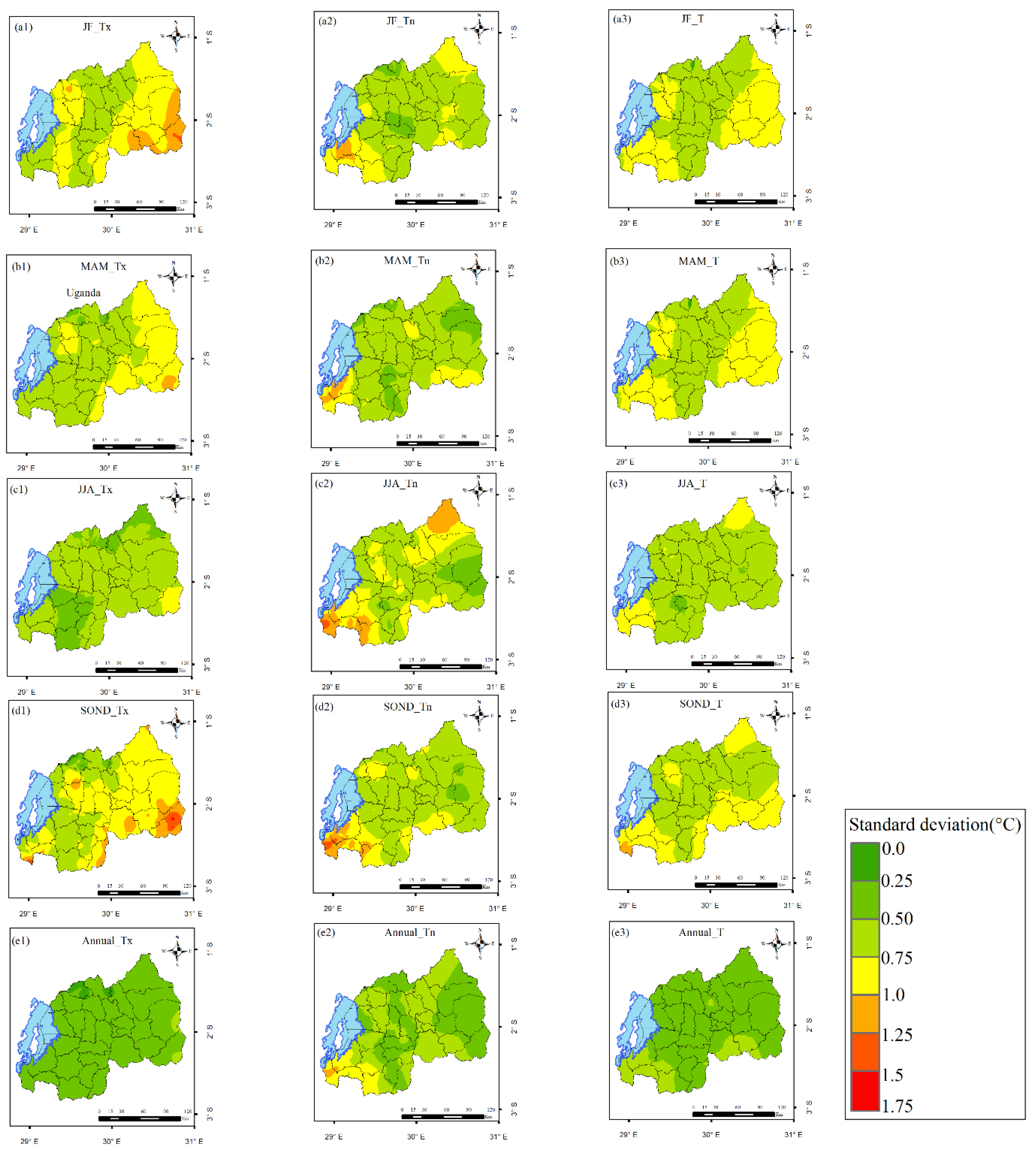
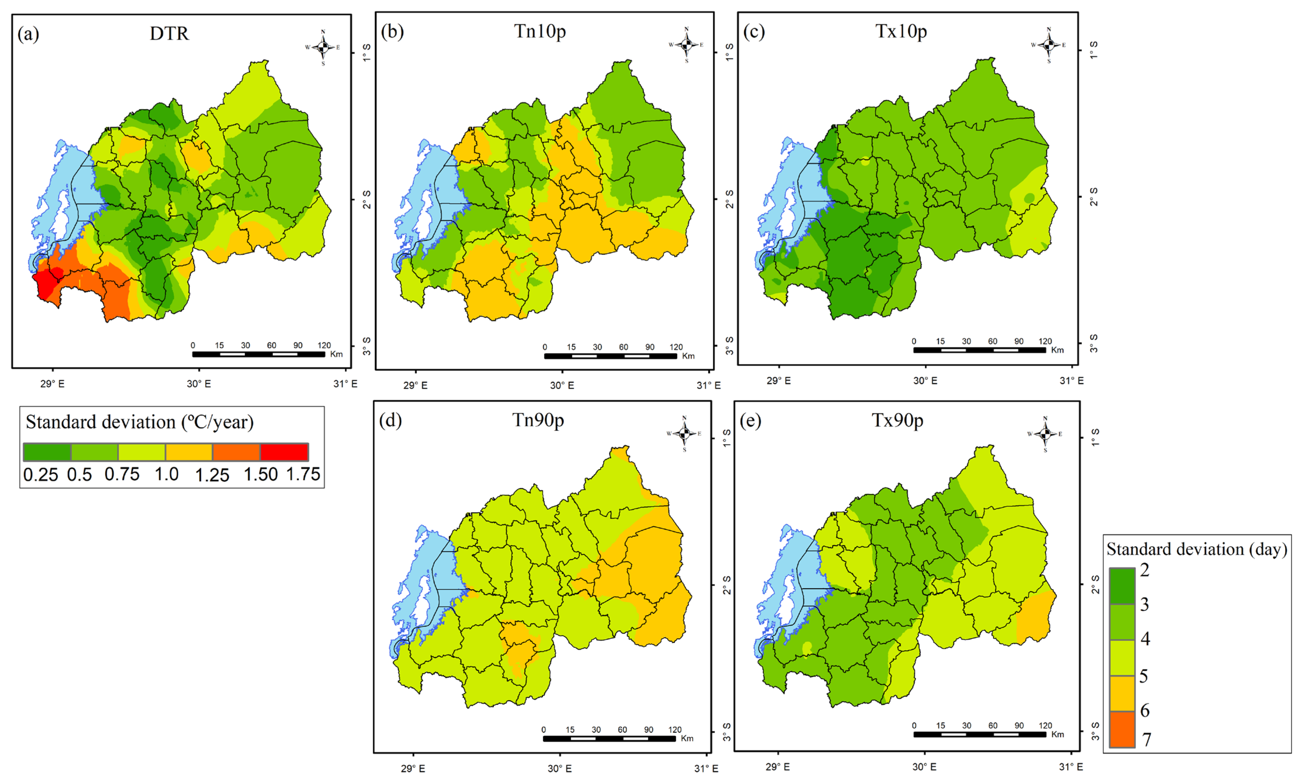
3.5. Variability in Temperatures and Extreme Indices

Figure 15 presents the spatial distributions of temporal variability of Tx, Tn, and T for JF, MAM, JJA, and SOND and the annual mean over Rwanda. In general, Tx represents the highest variability compared to Tn. Tx shows statistically significant high variability (1.4–1.6 °C) over the eastern and northwestern highlands in all seasons, except JJA. The two regions are important for the economy of the country as they constitute areas of intense agricultural activity. Tn country presents statistically significant high variability (1.2–1.4 °C) in the southwestern part of the country during all seasons, while it presents statistically significant high variability (1.0–1.2 °C) in the northeastern part of the country during JF and JJA seasons. The annual means of Tx and Tn indicate no statistically significant high value of variability is observed over the whole country. T shows that no statistically significant variability is observed for all seasons and the annual mean.

Figure 16 presents the spatial variability of DTR, Tn10p, Tx10p, Tn90p, and Tx90p. DTR shows statistically significant high variability (1.25–1.75 °C) in the southwestern parts compared to the south-central eastern part and a few areas of the northern highland (0.75–1.25 °C), while the remaining parts of the country indicate the lowest variability (0.25–0.75 °C). Tn10p shows higher variability ([5,6,7] days) than Tx10p (2–3 days), Tn90p (4–5 days), and Tx90p (3–4 days), especially in the area covering the central, south-western, south-central, and northwestern parts of Rwanda.

4. Discussion

Overall, temperatures decrease gradually with topography from the eastern to the western parts of the country in all seasons. Variations in temperature are primarily due to changes in cloud cover, rainfall, humidity, and winds. Temperatures follow the annual seasonal cycle. The difference in temperature between day and night is the maximum during JF and JJA and the minimum during MAM and SOND. The seasons of MAM and SOND correspond to the periods of crop growth. During those periods, statistically significant high positive trends of T were observed over some areas of great agricultural activity. Such an increase in T can affect crop production in the affected area by altering plant respiration rates and responses to biotic stressors [78].

Some studies have associated the higher rate of Tn compared to that of Tx with soil conditions, radiative cooling, and surface layer stability during the night [75,82]. The warming of surface temperature was linked to human-induced Greenhouse Gases [83,87]. In East Africa, the variability of temperature is in general associated with natural internal variability such as the El Nino Southern Oscillation as well as the Inter-decadal Pacific Oscillation [88,89,90]. In particular, the increased surface air temperature has led to the recently observed extreme dry events in the years of 2016 and 2017 over Rwanda. Rising temperatures may lead to increased evapotranspiration levels [91,92], impacting the water resources by decreasing water discharge, resulting in reduced hydropower generation [93]. In addition, it may intensify the drought conditions, leading to severe impacts on agricultural activities [26]. The observed strong variability of temperature over the eastern and northwestern highlands of Rwanda has negatively impacted the economy of the country as they constitute areas of intense agricultural activity [31].

Extreme temperature indices were found to be not coherent. The results obtained from country averages are in line with previous studies conducted over the East Africa region with the exception of Tx10p, which increases in Rwanda instead of decreasing [8,40,41,93,94,95,96,97]. The decrease in DTR has been observed in many parts of the world and was shown to be mainly related to the increase in Tn [98,99]. The changes in extreme temperature indices have been associated with the variation in convective rainfall events, cloud cover, increase in minimum temperature, or decrease in maximum temperature [100,101,102]. Several studies have revealed that the increase in DTR may affect human health by causing cardiovascular diseases and chronicle respiratory, resulting in low and high respiratory infections [43,103,104,105,106,107,108,109]. Zhou et al. [110] and Meinshausen et al. [111] have related changes in cold nights, cold days, warm nights, and warm days to climate change brought by human activities, including urbanization and industrialization, producing greenhouse gases [112,113,114,115]. The increase in warm nights, cold days, and warm days affects crop growth [95,116,117] and can influence the development and outbreak of new crop diseases [104]. Jang and Chun [103] have indicated that the rise in warm nights and warm days could induce significant impacts on sectors such as the energy necessitating high water for cooling, water supply by increasing freshwater need, and transportation by distortion of roads. The increase in temperature and drying conditions have resulted in increased drought in many places of the Earth [7,118,119,120,121,122,123,124]. During the last years, East Africa has experienced more recurrent, intense, and longer-lasting drought events [11,13,14,15,16,17,119], causing damage to infrastructure, water scarcity, drying of crops, famine, and food insecurity, leading to the frequent migrations of populations [17,18,19,20,21]. Recent observations have indicated that the eastern and southeastern parts of Rwanda have been experiencing rainfall deficits, resulting in severe droughts alternated by prolonged moderated drought. This made those areas vulnerable to water inaccessibility and food insecurity [17,26,30].

This study analyzed the trends and variability in the maximum, minimum, and mean temperatures and their associated extreme indices, as they have an impact on important key sectors of the economy such as agriculture, health, water resources, infrastructure, and energy. Another method of investigation recently developed can be used for comparison, such as the Innovative Trend Analysis methodology [125,126]. The results obtained will be useful in future studies to make a quantitative analysis of the effects of these trends and variables on these sectors. The obtained information will be useful in helping policy makers and decision makers integrate appropriate factors, taking into account mitigation and adaptation to climate change in planning for all sectorial levels.

5. Conclusions

In the present study, an analysis of the trends and variabilities of the maximum, minimum, and mean temperatures and their associated extreme indices was performed using the Modified Mann–Kendall test and the Theil–Sen estimator and the standard deviation, respectively. Statistically significant (α = 0.05) positive trends were observed for spatially averaged minimum temperature in JJA and SOND and for spatially averaged mean temperature in SOND. The maximum temperature presented higher variability than the minimum temperature and mean temperature countrywide. Diurnal temperature range and cold nights indicated a statistically significant (α = 0.05) decrease over the country, while warm days, cold days, and warm nights showed a statistically significant (α = 0.05). The diurnal temperature range showed a statistically significant (α = 0.05) high variability in the southwestern parts compared to the remaining parts of the country. Cold nights show higher variability than cold days, warm nights, and warm days, especially in the area covering the central, south-western, south-central parts, and the northwestern part of Rwanda.

These obtained results will be useful in future studies to make a quantitative analysis of the effects of these trends and variabilities on those sectors. They will serve to inform the community and policy decision making to take objective measures to prevent the impact of temperature increase and its variability on important economic sectors.

Some future directions of research can be mentioned: (i) investigate changes using other methods, i.e., Innovative Trend Analysis methodology recently developed [125,126] for comparison and (ii) recognize that drought is another effect of climate change in Rwanda. Some studies have recently been conducted on the East African region to determine the variability and trends in factors related to drought [127,128,129]. Further studies are still needed to investigate those factors to understand the effect of climate warming.

References

1. Brohan, P.; Kennedy, J.J.; Harris, I.; Tett, S.F.B.; Jones, P.D. Uncertainty estimates in regional and global observed temperature changes: A new data set from 1850. J. Geophys. Res. Atmos. 2006, 111, 1–21. [Google Scholar] [CrossRef]
2. IPCC. Climate Change 2007: Synthesis Report; Contribution of Working Groups I, II and III to the Fourth Assessment Report; IPCC: Geneva, Switzerland, 2007. [Google Scholar]
3. IPCC. Physical Science Basis: Summary for Policymakers. In Climate Change 2013; Contribution of Working Group I to the Fifth Assessment Report of the Intergovernmental Panel on Climate Change; Stocker, T.F., Qin, D., Plattner, G.-K., Tignor, M., Allen, S.K.J., Eds.; Cambridge University Press: Cambridge, UK; New York, NY, USA, 2013. [Google Scholar]
4. Bouwer, L.M. Have disaster losses increased due to anthropogenic climate change? Bull. Am. Meteorol. Soc. 2011, 92, 39–46. [Google Scholar] [CrossRef]
5. Comiso, J.C.; Perez, G.J.P.; Stock, L.V. Enhanced Pacific Ocean Sea surface temperature and its relation to typhoon Haiyan. J. Environ. Sci. Manag. 2015, 18, 1–10. [Google Scholar] [CrossRef]
6. Thomas, V.; López, R. Global Increase in Climate-Related Disasters. ADB Econ. Asian Dev. Bank (ADB), Manila, Work. Pap. Ser. 2015, 466, 1–33. [Google Scholar] [CrossRef]
7. IPCC. Climate Change 2021: The Physical Science Basis; Contribution of Working Group I to the Sixth Assessment Report of the Intergovernmental Panel on Climate Change; Masson-Delmotte, V., Zhai, P., Pirani, A., Connors, S.L., Péan, C., Berger, S., Caud, N., Chen, Y., Eds.; Cambridge University Press: Cambridge, UK, 2021. [Google Scholar] [CrossRef]
8. East Africa Hazards Watch “Cities Warming”. Available online: https://eahazardswatch.icpac.net/map/use/ (accessed on 26 June 2023).
9. Engelbrecht, F.; Adegoke, J.; Bopape, M.J.; Naidoo, M.; Garland, R.; Thatcher, M.; McGregor, J.; Katzfey, J.; Werner, M.; Ichoku, C.; et al. Projections of rapidly rising surface temperatures over Africa under low mitigation. Environ. Res. Lett. 2015, 10, 085004. [Google Scholar] [CrossRef]
10. WMO. World Meteorological Organization Commission for Climatology. In State of the Climate in Africa 2019; Report WMO-No.1253; World Meteorological Organisation: Geneva, Switzerland, 2020; 37p. [Google Scholar]
11. Gebrechorkos, S.H.; Hülsmann, S.; Bernhofer, C. Long-term trends in rainfall and temperature using high-resolution climate datasets in East Africa. Sci. Rep. 2019, 9, 11376. [Google Scholar] [CrossRef]
12. Daron, J.D. Regional Climate Messages: East Africa; Scientific Report from the CARIAA Adaptation at Scale in Semi-Arid Regions (ASSAR) Project; Springer: Cape Town, South Africa, 2014; pp. 1–30. [Google Scholar]
13. Russo, S.; Marchese, A.F.; Sillmann, J.; Immé, G. When will unusual heat waves become normal in a warming Africa? Environ. Res. Lett. 2016, 11, 054016. [Google Scholar] [CrossRef]
14. Herold, N.; Alexander, L.; Green, D.; Donat, M. Greater increases in temperature extremes in low versus high income countries. Environ. Res. Lett. 2017, 12, 10–13. [Google Scholar] [CrossRef]
15. Nashwan, M.S.; Shahid, S. Spatial distribution of unidirectional trends in climate and weather extremes in Nile River Basin. Theor. Appl. Climatol. 2019, 137, 1181–1199. [Google Scholar] [CrossRef]
16. Choi, Y.W.; Campbell, D.J.; Eltahir, E.A.B. Near-term regional climate change in East Africa. Clim. Dyn. 2022, 61, 961–978. [Google Scholar] [CrossRef]
17. Ayugi, B.; Tan, G.; Niu, R.; Dong, Z.; Ojara, M.; Mumo, L.; Babaousmail, H.; Ongoma, V. Evaluation of Meteorological Drought and Flood Scenarios over Kenya, East Africa. Atmosphere 2020, 11, 307. [Google Scholar] [CrossRef]
18. Abebe, M.A. Climate Change, Gender Inequality, and Migration in East Africa. Washingt. J. Environ. Law Policy 2014, 4, 104–140. [Google Scholar]
19. Mueller, V.; Sheriffc, G.; Dou, X.; Gray, C. Temporary migration and climate variation in Eastern Africa. World Dev. 2020, 126, 104704. [Google Scholar] [CrossRef]
20. Bannor, F.; Magambo, I.H.; Mahabir, J.; Tshitaka, J.-L.M. Interdependence between climate change and migration: Does Agriculture, geography and development level matter in sub-Saharan Africa? SAJE 2022, 91, 141–160. [Google Scholar] [CrossRef]
21. Richardson, K.; Calow, R.; Pichon, F.; New, S.; Osborne, R. Climate Risk Report for the East Africa Region; Met Office, ODI, FCDO: Cape Town, South Africa, 2022. [Google Scholar]
22. Zhou, G.; Minakawa, N.; Githeko, A.K.; Yan, G. Association between climate variability and malaria epidemics in the East Africian highlands. Proc. Natl. Acad. Sci. USA 2004, 101, 2375–2380. [Google Scholar] [CrossRef] [PubMed]
23. Safari, B. Trend Analysis of the Mean Annual Temperature in Rwanda during the Last Fifty-Two Years. J. Environ. Prot. 2012, 3, 538–551. [Google Scholar] [CrossRef]
24. Safari, B. A review of energy in Rwanda. Renew. Sustain. Energy Rev. 2010, 14, 524–529. [Google Scholar] [CrossRef]
25. Li, C.; Yang, M.; Li, Z.; Wang, B. How will Rwandan land use/land cover change under high population pressure and changing climate? Appl. Sci. 2021, 11, 5376. [Google Scholar] [CrossRef]
26. Uwimbabazi, J.; Jing, Y.; Iyakaremye, V.; Ullah, I.; Ayugi, B. Observed Changes in Meteorological Drought Events during 1981–2020 over Rwanda, East Africa. Sustainability 2022, 14, 1519. [Google Scholar] [CrossRef]
27. Loevinsohn, M.E. Climatic warming and increased malaria incidence in Rwanda. Lancet 1994, 343, 714–718. [Google Scholar] [CrossRef]
28. Henninger, S.M. Local climate changes and the spread of malaria in Rwanda. Health 2013, 5, 728–734. [Google Scholar] [CrossRef]
29. Maniragaba, A.; Muse, S.G.; Benjamin, M.N.; Kato, N.J. Impact of Climate Variation on Malaria Incidence in Rwandan Highland. East African J. Sci. Technol. 2018, 8, 75–76. [Google Scholar]
30. Muneza, L. Droughts and Floodings Implications in Agriculture Sector in Rwanda: Consequences of Global Warming. In The Nature, Causes, Effects and Mitigation of Climate Change on the Environment; IntechOpen: London, UK, 2016; p. 11. [Google Scholar] [CrossRef]
31. Hunter, R.; Crespo, O.; Coldrey, K.; Cronin, K.; New, M. Research Highlights—Climate Change and Future Crop Suitability in Rwanda; Undertaken in support of Adaptation for Smallholder Agriculture Programme’ (ASAP) Phase 2; International Fund for Agricultural Development (IFAD): Rome, Italy; University of Cape Town: Cape Town, South Africa, 2020. [Google Scholar]
32. Easterling, D.R.; Meehl, G.A.; Parmesan, C.; Changnon, S.A.; Karl, T.R.; Mearns, L. Climate extremes: Observations, modelling and impacts. Science 2000, 289, 2068–2074. [Google Scholar] [CrossRef] [PubMed]
33. Meehl, G.A.; Karl, T.; Easterling, D.R.; Changnon, S.; Pielke, R.; Changnon, D., Jr.; Evans, J.; Groisman, P.Y.; Knutson, T.R.; Knukel, K.E.; et al. An introduction to trends in extreme weather and climate events: Observations, socioeconomic impacts, terrestrial ecological impacts, and model projections. Bull. Am. Meteorol. Soc. 2000, 81, 413–416. [Google Scholar] [CrossRef]
34. Walther, G.R.; Post, E.; Convey, P.; Menzel, A.; Parmesan, C.; Beebee, T.J.C.; Fromentin, J.M.; Hoegh Guldberg, O.; Bairlein, F. Ecological responses to recent climate change. Nature 2002, 416, 389–395. [Google Scholar] [CrossRef] [PubMed]
35. Intergovernmental Panel on Climate Change. Managing the Risks of Extreme Events and Disasters to Advance Climate Change Adaptation; A Special Report of Working Groups I and II of the Intergovernmental Panel on Climate Change; Field, C.B., Barros, V., Stocker, T.F., Qin, D., Dokken, D.J., Ebi, K.L., Mastrandrea, M.D., Mach, K.J., Plattner, G.-K., Allen, S.K., et al., Eds.; Cambridge University Press: Cambridge, UK; New York, NY, USA, 2012. [Google Scholar]
36. Revadekar, J.V.; Kothawale, D.R.; Patwardhan, S.K.; Pant, G.B.; Rupa Kumar, K. About the observed and future changes in temperature extremes over India. Nat. Hazards. 2012, 60, 1133–1155. [Google Scholar] [CrossRef]
37. Stephenson, D.B. Definition, diagnosis, and origin of extreme weather and climate events. In Climate Extremes and Society; Diaz, H.F., Murnane, R.J., Eds.; Cambridge University Press: New York, NY, USA, 2008; pp. 11–23. [Google Scholar]
38. Alexander, L.V.; Zhang, X.; Peterson, T.C.; Caesar, J.; Gleason, B.; Klein Tank, A.; Haylock, M.; Collins, D.; Trewin, B.; Rahimzadeh, F.; et al. Global observed changes in daily climate extremes of temperature and precipitation. J. Geophys. Res. 2006, 111, D05109. [Google Scholar] [CrossRef]
39. Caeser, J.; Alexander, L.; Vose, R. Large-scale changes in observed daily maximum and minimum temperatures: Creation and analysis of a new gridded dataset. J. Geophys. Res. 2006, 111, D05101. [Google Scholar] [CrossRef]
40. Ngaina, J.; Mutai, B. Observational evidence of climate change on extreme events over East Africa. Glob. Meteorol. 2013, 2, e2. [Google Scholar] [CrossRef]
41. Omondi PA, O.; Awange, J.L.; Forootan, E.; Ogallo, L.A.; Barakiza, R.; Girmaw, G.B.; Fesseha, I.; Kululetera, V.; Kilembe, C.; Mbati, M.M.; et al. Changes in temperature and precipitation extremes over the Greater Horn of Africa region from 1961 to 2010. Int. J. Climatol. 2014, 34, 1262–1277. [Google Scholar] [CrossRef]
42. Ngarukiyimana, J.P.; Fu, Y.; Sindikubwabo, C.; Nkurunziza, I.F.; Ogou, F.K.; Vuguziga, F.; Ogwang, B.A.; Yang, Y. Climate Change in Rwanda: The Observed Changes in Daily Maximum and Minimum Surface Air Temperatures during 1961–2014. Front. Earth Sci. 2021, 9, 619512. [Google Scholar] [CrossRef]
43. Cheng, J.; Xu, Z.; Zhu, R.; Wang, X.; Jin, L.; Song, J.; Su, H. Impact of diurnal temperature range on human health: A systematic review. Int. J. Biometeorol. 2014, 58, 2011–2024. [Google Scholar] [CrossRef] [PubMed]
44. Lei, L.; Bao, J.; Guo, Y.; Wang, Q.; Peng, J.; Huang, C. Effects of diurnal temperature range on first-ever strokes in different seasons: A time-series study in Shenzhen, China. BMJ 2020, 10, e033571. [Google Scholar] [CrossRef] [PubMed]
45. Bastin, J.F.; Clark, E.; Elliott, T.; Hart, S.; Van Den Hoogen, J.; Hordijk, I.; Ma, H.; Majumder, S.; Manoli, G.; Maschler, J.; et al. Understanding climate change from a global analysis of city analogues. PLoS ONE 2019, 14, e0224120. [Google Scholar] [CrossRef]
46. Rwanda. National Adaptation Programmes of Action for Climate Change; Ministry of Lands, Environment, Forestry, Water and Mines: Kigali, Rwanda, 2006.
47. Rwanda. Green Growth and Climate Resilience-National Strategy on Climate Change and Low Carbon Development; Ministry of Natural Resources: Kigali, Rwanda, 2011.
48. Rwanda. Evaluation of the Green Growth and Climate Resilience Strategy Implementation; Ministry of Environment: Kigali, Rwanda, 2018.
49. Rwanda. National Environment and Climate Change Policy; Ministry of Environment: Kigali, Rwanda, 2019.
50. Rwanda. Rwanda’s Revised Nationally Determined Contributions—NDCs; Ministry of Environment: Kigali, Rwanda, 2020.
51. Clay, N.; King, B. Smallholders’ uneven capacities to adapt to climate change amid Africa’s ‘green revolution’: Case study of Rwanda’s crop intensification program. World Dev. 2019, 116, 1–14. [Google Scholar] [CrossRef]
52. Kim, S.K.; Marshall, F.; Dawson, N.M. Revisiting Rwanda’s agricultural intensification policy: Benefits of embracing farmer heterogeneity and crop-livestock integration strategies. Food Secur. 2022, 14, 637–656. [Google Scholar] [CrossRef]
53. Rwanda. Revised Green Growth and Climate Resilience National Strategy for Climate Change and Low Carbon Development & Acknowledgements; Ministry of Environment: Kigali, Rwanda, 2022.
54. Trevor, M.L. The Impacts of Climate Change: A Comprehensive Study of Physical, Biophysical, Social and Political Issues; Elsevier: Amsterdam, The Netherlands, 2021; pp. 547–557. ISBN 978-0-12-822373-4. [Google Scholar] [CrossRef]
55. WMO. Report of the CCl/CLIVAR Expert Team on Climate Change Detection, Monitoring and Indices (ETCCDMI); WMO-TD No. 1205; World Meteorological Organization: Geneva, Switzerland, 2004. [Google Scholar]
56. White, J.W.C.; Alley, R.B.; Archer, D.E.; Barnosky, A.D.; Dunlea, E.; Foley, J.; Fu, R.; Holland, M.M.; Lozier, M.S.; Schmitt, J.; et al. Abrupt Impacts of Climate Change: Anticipating Surprises; The National Academies Press: Washington, DC, USA, 2013. [Google Scholar] [CrossRef]
57. STAP. Strengthening Monitoring and Evaluation of Climate Change Adaptation: A STAP Advisory Document; Global Environment Facility: Washington, DC, USA, 2017. [Google Scholar]
58. FAO. Tracking Adaptation in Agricultural Sectors: Climate Change Adaptation Indicators; Food and Agriculture Organization of the United Nations: Rome, Italy, 2018. [Google Scholar] [CrossRef]
59. Henninger, M.S. Does the global warming modify the local Rwandan climate? Nat. Sci. 2013, 5, 124–129. [Google Scholar] [CrossRef]
60. National Institute of Statistics of Rwanda. Main Indicators: 5th Rwandan Population and Housing Census (PHC); National Institute of Statistics of Rwanda: Kigali, Rwanda, 2023. [Google Scholar]
61. Dinku, T.; Hailemariam, K.; Maidment, R.; Tarnavsky, E.; Connor, S. Combined use of satellite estimates and rain gauge observations to generate high-quality historical rainfall time series over Ethiopia. Int. J. Climatol. 2014, 34, 2489–2504. [Google Scholar] [CrossRef]
62. Siebert, A.; Dinku, T.; Vuguziga, F.; Twahirwa, A.; Kagabo, M.D.; DelCorral, J.; Robertson, A.W. Evaluation of ENACTS-Rwanda: A new multi-decade, highresolution rainfall and temperature data set—Climatology. Int. J. Climatol. 2019, 34, 1262–1277. [Google Scholar] [CrossRef]
63. Karl, T.; Nicholls, N.; Ghazi, A. CLIVAR/RCOS/WMO Workshop on Indices and Indicators for Climate Extremes. Clim. Change 1999, 42, 3–7. [Google Scholar] [CrossRef]
64. Zhang, X.; Alexander, L.; Hegerl, G.C.; Jones, P.; Tank, A.K.; Peterson, T.C.; Trewin, B.; Zwiers, F.W. Indices for monitoring changes in extremes based on daily temperature and precipitation data. Wiley Interdiscip. Rev. Clim. Change 2011, 2, 851–870. [Google Scholar] [CrossRef]
65. Tank, A.M.G.K.; Zwiers, F.W.; Zhang, X. Guidelines on Analysis of Extremes in a Changing Climate in Support of Informed Decisions for Adaptation; Climate Data and Monitoring Rep.WCDMP 72; WMO-TD 1500, no. 72; World Meteorological Organization: Geneva, Switzerland, 2009; 56p. [Google Scholar]
66. Zhang, X.; Yang, F. RClimDex (1.0) User Manual; Climate Research Branch Environment Canada: Downsview, ON, Canada, 2004; pp. 1–23. [Google Scholar]
67. Folland, C.K.; Christy, J.R.; Clarke, R.A.; Gruza, G.V.; Jouzel, J.; Mann, M.E.; Oerlemans, J.; Salinger, M.J.; Wang, S.-W. Observed Climate variability and Climate Change. In Climate 2001: The Scientific Basis; Cambrige University Press, Cambrdge, 2001; p. 108.
68. Sneyers, R. On the Statistical Analysis of Series of Obervations; WMO Technical Note 143; WMO No. 415, TP-103; World Meteorological Organization: Geneva, Switzerland, 1990. [Google Scholar]
69. Tan, C.; Yang, J.; Li, M. Temporal-Spatial Variation of Drought Indicated by SPI and SPEI in Ningxia Hui Autonomous Region, China. Atmosphere 2015, 6, 1399–1421. [Google Scholar] [CrossRef]
70. Hamed, K.H.; Rao, A.R. A modified Mann-Kendall trend test for autocorrelated data. J. Hydrol. 1998, 204, 182–196. [Google Scholar] [CrossRef]
71. Serrano, A.; Mateos, V.L.; Garcia, J.A. Trend analysis of monthly precipitation over the Iberian Peninsula for the Period 1921–1995. Phys. Chem. Earth 1999, 24, 85–90. [Google Scholar] [CrossRef]
72. Yue, S.; Pilon, P.; Phinney, B. Canadian streamflow trend detection: Impacts of serial and cross-correlation. Hydrol. Sci. J. 2003, 48, 51–63. [Google Scholar] [CrossRef]
73. Novotny, E.V.; Stefan, H.G. Stream flow in Minnesota: Indicator of Climate Change. J. Hydrol. 2007, 334, 319–333. [Google Scholar] [CrossRef]
74. Datta, P.; Das, S. Analysis of long-term seasonal and annual temperature trends in North Bengal, India. Spat. Inf. Res. 2019, 27, 475–496. [Google Scholar] [CrossRef]
75. Ahmed, K.; Shahid, S.; Ali, R.O.; Bin Harun, S.; Wang, X.J. Evaluation of the performance of gridded precipitation products over Balochistan Province, Pakistan. Desalin. Water Treat. 2017, 79, 73–86. [Google Scholar] [CrossRef]
76. Taxak, A.K.; Murumkar, A.R.; Arya, D.S. Long term spatial and temporal rainfall trends and homogeneity analysis in Wainganga basin, Central India. Weather. Clim. Extrem. 2014, 4, 50–61. [Google Scholar] [CrossRef]
77. Mahrt, L. Stably stratified atmospheric boundary layers. Annu. Rev. Fluid Mech. 2014, 46, 23–45. [Google Scholar] [CrossRef]
78. Das, S.; Datta, P.; Sharma, D.; Goswami, K. Trends in Temperature, Precipitation, Potential Evapotranspiration, and Water Availability across the Teesta River Basin under 1.5 and 2 °C Temperature Rise Scenarios of CMIP6. Atmosphere 2022, 13, 941. [Google Scholar] [CrossRef]
79. Arun, M.; Sananda, K.; Anirban, M. Rainfall Trend Analysis by Mann-Kendall Test: A Case Study of North-Eastern Part of Cuttack District, Orissa. JGEE 2012, 2, 70–78. [Google Scholar]
80. Sen, P.K. Estimates of the Regression Coefficient Based on Kendall’s Tau. J. Am. Stat. Assoc. 1968, 63, 1379–1389. [Google Scholar] [CrossRef]
81. Theil, H. A rank-invariant method of linear and polynomial regression analysis, part 3. In Henri Theil’s Contributions to Economics and Econometrics; Springer: Dordrecht, The Netherlands, 1992. [Google Scholar]
82. Chechin, D.G.; Makhotina, I.A.; Lüpkes, C.; Makshtas, A.P. Effect of wind speed and leads on clear-sky cooling over Arctic Sea ice during polar night. J. Atmos. Sci. 2019, 76, 2481–2503. [Google Scholar] [CrossRef]
83. Allabakash, S.; Lim, S. Anthropogenic influence of temperature changes across East Asia using CMIP6 simulations. Sci. Rep. 2022, 12, 11896. [Google Scholar] [CrossRef]
84. Weber, D.; Englund, E. Evaluation and comparison of spatial interpolators. Math Geol. 1992, 24, 381–391. [Google Scholar] [CrossRef]
85. Weber, D.D.; Englund, E.J. Evaluation and comparison of spatial interpolators II. Math Geol. 1994, 26, 589–603. [Google Scholar] [CrossRef]
86. Setianto, A.; Triandini, T. Comparison of Kriging and Inverse Distance Weighted (IDW) Interpolation Methods in Lineament Extraction and Analysis. J. SE Asian Appl. Geol. 2013, 5, 21–29. [Google Scholar] [CrossRef]
87. Lu, C.; Sun, Y.; Zhang, X. Anthropogenic Influence on the Diurnal Temperature Range since 1901. J. Clim. 2022, 35, 3583–3598. [Google Scholar] [CrossRef]
88. Gu, G.; Adler, R.F. Interdecadal variability/long-term changes in global precipitation patterns during the past three decades: Global warming and/or pacific decadal variability? Clim. Dyn. 2013, 40, 3009–3022. [Google Scholar] [CrossRef]
89. Lyon, B. Seasonal drought in the Greater Horn of Africa and its recent increase during the March-May long rains. J. Clim. 2014, 27, 7953–7975. [Google Scholar] [CrossRef]
90. Dai, A. Future Warming Patterns Linked to Today’s Climate Variability. Sci. Rep. 2016, 6, 6–11. [Google Scholar] [CrossRef]
91. Bunyasi, M. Vulnerability of Hydro-Electric Energy Resources in Kenya Due to Climate Change Effects: The Case of the Seven Forks Project. J. Agric. Environ. Sci. 2012, 1, 36–49. [Google Scholar]
92. Machina, B.M.; Sharma, S. Assessment of Climate Change Impact on Hydropower Generation: A Case Study of Nigeria. Int. J. Eng. Technol. Sci. Res. 2017, 4, 753–762. [Google Scholar]
93. Kachaje, O.; Kasulo, V.; Chavula, G. The potential impacts of climate change on hydropower: An assessment of Lujeri micro hydropower scheme, Malawi. Afr. J. Environ. Sci. Technol. 2016, 10, 476–484. [Google Scholar] [CrossRef]
94. Owoyesigire, B.; Mpairwe, D.; Ericksen, P.; Peden, D. Trends in variability and extremes of rainfall and temperature in the cattle corridor of Uganda. Uganda J. Agric. Sci. 2016, 17, 231–244. [Google Scholar] [CrossRef]
95. Mekasha, A.; Tesfaye, K.; Duncan, A.J. Trends in daily observed temperature and precipitation extremes over three Ethiopian eco-environments. Int. J. Climatol. 2014, 34, 1990–1999. [Google Scholar] [CrossRef]
96. Gebrechorkos, S.H.; Hülsmann, S.; Bernhofer, C. Changes in temperature and precipitation extremes in Ethiopia, Kenya, and Tanzania. Int. J. Climatol. 2019, 39, 18–30. [Google Scholar] [CrossRef]
97. Chang’a, L.B.; Kijazi, A.L.; Luhunga, P.M.; Ng’ongolo, H.K.; Mtongor, H.I. Spatial and Temporal Analysis of Rainfall and Temperature Extreme Indices in Tanzania. Atmos. Clim. Sci. 2017, 7, 525–539. [Google Scholar] [CrossRef]
98. Easterling, D.R.; Horton BJones, P.D.; Peterson, T.C.; Karl, R.R.; Parker, D.E.; Salinger MJFolland, V.C.L. Maximum and Minimum Temperature trends for the globe. Science 1997, 277, 364–367. [Google Scholar] [CrossRef]
99. Vose, R.S.; Easterling, D.R.; Gleason, B. Maximum and Minimum Temperature Trends for the Globe: An Update Through 2004. Geophys. Res. Lett. 2005, 32, L23822. [Google Scholar] [CrossRef]
100. Camberlin, P. Temperature trends and variability in the Greater Horn of Africa: Interactions with precipitation. Clim. Dyn. 2017, 48, 477–498. [Google Scholar] [CrossRef]
101. Dike, V.N.; Lin, Z.; Wang, Y.; Nnamchi, H. Observed trends in diurnal temperature range over Nigeria. Atmos. Ocean. Sci. Lett. 2019, 12, 131–139. [Google Scholar] [CrossRef]
102. Zhou, L.; Dai, A.; Dai, Y.; Vose, R.S.; Zou, C.Z.; Tian, Y.; Chen, H. Spatial dependence of diurnal temperature range trends on precipitation from 1950 to 2004. Clim. Dyn. 2009, 32, 429–440. [Google Scholar] [CrossRef]
103. Wang, Z.; Zhou, Y.; Luo, M.; Yang, H.; Xiao, S.; Huang, X.; Ou, Y.; Zhang, Y.; Duan, X.; Hu, W.; et al. Association of diurnal temperature range with daily hospitalization for exacerbation of chronic respiratory diseases in 21 cities, China. Respir. Res. 2020, 21, 251. [Google Scholar] [CrossRef] [PubMed]
104. Jang, J.Y.; Chun, B.C. Effect of diurnal temperature range on emergency room visits for acute upper respiratory tract infections. Environ. Health Prev. Med. 2021, 26, 55. [Google Scholar] [CrossRef] [PubMed]
105. Carreras, H.; Zanobetti, A.; Koutrakis, P. Effect of daily temperature range on respiratory health in Argentina and its modification by impaired socio-economic conditions and PM10 exposures. Environ. Pollut. 2015, 206, 175–182. [Google Scholar] [CrossRef]
106. King’uyu, S.M.; Ogallo, L.A.; Anyamba, E.K. Recent trends of minimum and maximum surface temperatures over Eastern Africa. J. Clim. 2000, 13, 2876–2886. [Google Scholar] [CrossRef]
107. Lim, Y.H.; Hong, Y.C.; Kim, H. Effects of diurnal temperature range on cardiovascular and respiratory hospital admissions in Korea. Sci. Total Environ. 2012, 15, 417–418. [Google Scholar] [CrossRef]
108. Wang, M.Z.; Zheng, S.; He, S.L.; Li, B.; Teng, H.J.; Wang, S.G.; Yin, L.; Shang, K.Z.; Li, T.S. The association between diurnal temperature range and emergency room admissions for cardiovascular, respiratory, digestive and genitourinary disease among the elderly: A time series study. Sci. Total Environ. 2013, 1, 456–457. [Google Scholar] [CrossRef]
109. Zheng, S.; Wang, M.; Li, B.; Wang, S.; He, S.; Yin, L.; Shang, K.; Li, T. Gender, Age and Season as Modifiers of the Effects of Diurnal Temperature Range on Emergency Room Admissions for Cause-Specific Cardiovascular Disease among the Elderly in Beijing. Int. J. Environ. Res. Public Health 2016, 13, 447. [Google Scholar] [CrossRef] [PubMed]
110. Meinshausen, M.; Meinshausen, N.; Hare, W.; Raper, S.C.B.; Frieler, K.; Knutti, R.; Frame, D.J.; Allen, M.R. Greenhouse-gas emission targets for limiting global warming to 2 °C. Nature 2009, 458, 1158–1162. [Google Scholar] [CrossRef]
111. Unger, J. Intra-urban relationship between surface geometry and urban heat island: Review and new approach. Clim. Res. 2004, 27, 253–264. [Google Scholar] [CrossRef]
112. Hu, W.; Zhou, W.; He, H. The effect of land-use intensity on surface temperature in the dongting lake area, China. Adv. Meteorol. 2015, 2015, 632151. [Google Scholar] [CrossRef]
113. Chen, L.; Dirmeyer, P.A. Distinct Impacts of Land Use and Land Management on Summer Temperatures. Front. Earth Sci. 2020, 8, 245. [Google Scholar] [CrossRef]
114. Lu, Y.; Yue, W.; Huang, Y. Effects of land use on land surface temperature: A case study of Wuhan, China. Int. J. Environ. Res. Public Health 2021, 18, 9987. [Google Scholar] [CrossRef] [PubMed]
115. Marigi, S.N.; Njogu, A.K.; Githungo, W.N. Trends of Extreme Temperature and Rainfall Indices for Arid and Semi-Arid Lands of South Eastern Kenya. J. Geosci. Environ. Prot. 2016, 4, 158. [Google Scholar] [CrossRef]
116. Leng, G.; Tang, Q.; Rayburg, S. Climate change impacts on meteorological, agricultural and hydrological droughts in China. Glob. Planet. Chang. 2015, 126, 23–34. [Google Scholar] [CrossRef]
117. Sheffield, J.; Wood, E.F.; Roderick, M.L. Little change in global drought over the past 60 years. Nature 2012, 491, 435–438. [Google Scholar] [CrossRef]
118. Feng, T.; Jianjun, W.; Leizhen, L.; Song, L.; Jianhua, Y.; Wenhui, Z.; Qiu, S. Exceptional Drought across Southeastern Australia Caused by Extreme Lack of Precipitation and Its Impacts on NDVI and SIF in 2018. Remote Sens. 2020, 12, 54. [Google Scholar] [CrossRef]
119. Agutu, N.O.; Awange, J.L.; Zerihun, A.; Ndehedehe, C.E.; Kuhn, M.; Fukuda, Y. Assessing multi-satellite remote sensing, reanalysis, and land surface models’ products in characterizing agricultural drought in East Africa. Remote Sens. Environ. 2017, 194, 287–302. [Google Scholar] [CrossRef]
120. REMA. Assessment of Climate Change Vulnerability in Rwanda—2018; REMA: Kigali, Rwanda, 2019. [Google Scholar]
121. Polong, F.; Chen, H.; Sun, S.; Ongoma, V. Temporal and spatial evolution of the standard precipitation evapotranspiration index (SPEI) in the Tana River Basin, Kenya. Theor. Appl. Climatol. 2019, 138, 777–792. [Google Scholar] [CrossRef]
122. Mutsotso, R.B.; Sichangi, A.W.; Makokha, G.O. Spatio-Temporal Drought Characterization in Kenya from 1987 to 2016. Adv. Remote Sens. 2018, 7, 125–143. [Google Scholar] [CrossRef]
123. Kew, S.F.; Philip, S.Y.; Hauser, M.; Hobbins, M.; Wanders, N.; van Oldenborgh, G.J.; van der Wiel, K.; Veldkamp, T.I.E.; Kimutai, J.; Funk, C.; et al. Impact of precipitation and increasing temperatures on drought trends in eastern Africa. Earth Syst. Dyn. 2021, 12, 17–35. [Google Scholar] [CrossRef]
124. Khodzhimetov, T.A. Measuring devices for monitoring parodontium resistance and endurance towards chewing load. Biomed. Eng. 1997, 31, 56–58. [Google Scholar] [CrossRef]
125. Birpınar, M.E.; Kızılöz, B.; Şişman, E. Classic trend analysis methods’ paradoxical results and innovative trend analysis methodology with percentile ranges. Theor. Appl. Climatol. 2023, 153, 1–18. [Google Scholar] [CrossRef]
126. Alashan, S. Combination of modified Mann-Kendall method and Şen innovative trend analysis. Eng. Rep. 2020, 2, e12131. [Google Scholar] [CrossRef]
127. Lobell, D.B.; Field, C.B. Global scale climate-crop yield relationships and the impacts of recent warming. Environ. Res. Lett. 2007, 2, 014002. [Google Scholar] [CrossRef]
128. Christiansen, D.E.; Markstrom, S.L.; Hay, L.E. Impacts of climate change on the growing season in the United States. Earth Interact. 2011, 15, 1–17. [Google Scholar] [CrossRef]
129. Pita-Díaz, O.; Ortega-Gaucin, D. Analysis of anomalies and trends of climate change indices in Zacatecas, Mexico. Climate 2020, 8, 55. [Google Scholar] [CrossRef]
Figure 1. The elevation map of Rwanda (a) and the grid covering the study area (b).
Atmosphere 14 01449 g001
Figure 2. Spatial distribution of long-term mean of Tx, Tn, and T over Rwanda during the period of 1983–2022 expressed in °C. Tx for JF (a1), Tx for MAM (a2), Tx for JJA (a3), Tx for SOND (a4), Tx for mean annual (a5),Tn for JF (b1), Tn for MAM (b2), Tn for JJA (b3), Tn for SOND (b4), Tn for mean annual (b5), T for JF (c1), T for MAM (c2), T for JJA (c3), T for SOND (c4), T for mean annual (c5), (Computed from the data used in this study, obtained from Rwanda Meteorology Agency).
Atmosphere 14 01449 g002
Figure 3. Spatial distribution of trends for Tx, Tn, and T over Rwanda during the period of 1983–2022 expressed in °C/decade. Tx for JF (a1), Tn for JF (a2), T for JF (a3), Tx for MAM (b1), Tn for MAM (b2), T for MAM (b3), Tx for JJA (c1), Tn for JJA (c2), T for JJA (c3), Tx for SOND (d1), Tn for SOND (d2), T for SOND (d3), mean annual Tx (e1), mean annual Tn (e2), and mean annual T (e3). Trend slope in °C/decade (obtained by multiplying by 10 the computed trend slope in °C/year using the MMK method). Areas with statistically significant positive trends are indicated with + sign, and areas with statistically significant negative trends are indicated with − sign.
Atmosphere 14 01449 g003
Figure 4. Decadal differences of Tx for JF, MAM, JJA, SOND, and the annual mean with reference to the period of 1983–1992. Tx for JF (1993–2002) (a1), Tx for JF (2003–2012) (a2), Tx for JF (2013–2022) (a3), Tx for MAM (1993-2002) (b1), Tx for MAM (2003–2012) (b2), Tx for MAM (2013–2022) (b3), Tx for JJA (1993–2002) (c1), Tx for JJA (2003–2012) (c2), Tx for JJA (2013–2022) (c3), Tx for SOND (1993–2002) (d1), Tx for SOND (2003–2012) (d2), Tx for SOND (2013–2022) (d3), annual Tx (1993–2002) (e1), annual Tx (2003–2012) (e2), and for annual Tx (2013–2022) (e3).
Atmosphere 14 01449 g004
Figure 5. Decadal differences of Tn for JF, MAM, JJA, SOND, and the annual mean with reference to the period of 1983–1992. Tn for JF (1993–2002) (a1), Tn for JF (2003–2012) (a2), Tn for JF (2013–2022) (a3), Tn for MAM (1993–2002) (b1), Tn for MAM (2003–2012) (b2), Tn for MAM (2013–2022) (b3), Tn for JJA (1993–2002) (c1), Tn for JJA (2003–2012) (c2), Tn for JJA (2013–2022) (c3), Tn for SOND (1993–2002) (d1), Tn for SOND (2003–2012) (d2), Tn for SOND (2013–2022) (d3), annual Tn (1993–2002) (e1), annual Tn (2003–2012) (e2), and annual Tn (2013–2022) (e3).
Atmosphere 14 01449 g005
Figure 6. Decadal differences of T for JF, MAM, JJA, SOND, and the annual mean with reference to the period of 1983–1992. T for JF (1993–2002) (a1), T for JF (2003–2012) (a2), T for JF (2013–2022) (a3), T for MAM (1993–2002) (b1), T for MAM (2003–2012) (b2), T for MAM (2013–2022) (b3), T for JJA (1993–2002) (c1), T for JJA (2003–2012) (c2), T for JJA (2013–2022) (c3), T for SOND (1993–2002) (d1), T for SOND (2003–2012) (d2), T for SOND (2013–2022) (d3), annual T (1993–2002) (e1), annual T (2003–2012) (e2), and annual T (2013–2022) (e3).
Atmosphere 14 01449 g006
Figure 7. Spatial distribution of long-term mean of DTR (a) expressed in °C, Tn10p (b); Tx10p (c); Tn90p (d); and Tx90p (e) expressed in days over Rwanda for the period 1983–2022. Legend is common for Tn10p, Tn90p, Tx10p, and Tx90p.
Atmosphere 14 01449 g007
Figure 8. Spatial distribution of trends of DTR (a) expressed in °C/decade, Tn10p (b); Tx10p (c); Tn90p (d); and Tx90p (e) expressed in days/decade over Rwanda during the period of 1983–2022. “Trend slope in °C/decade (obtained by multiplying by 10 the computed trend slope in °C/year by the MMK method) for DRT” and “Trend slope in Days/decade (obtained by multiplying by 10 the computed trend slope in Days/year by the MMK method) for Tn10p, Tn90p, Tx10p, and Tx90p”. Areas with statistically significant positive trends are indicated with + sign, and areas with statistically significant negative trends are indicated with − sign. Legend is common for Tn10p, Tn90p, Tx10p, and Tx90p.
Atmosphere 14 01449 g008
Figure 9. Decadal spatial distribution of DTR expressed in °C over Rwanda for the period of 1983–2022. The first decade (1983–1992) (a), the second decade (1993–2002) (b), the third decade (2003–2012) (c), and the fourth decade (2013–2022) (d).
Atmosphere 14 01449 g009
Figure 10. Decadal spatial distribution of Tn10p expressed in day/year over Rwanda for the period of 1983–2022. The first decade (1983–1992) (a), the second decade (1993–2002) (b), the third decade (2003–2012) (c), and the fourth decade (2013–2022) (d).
Atmosphere 14 01449 g010
Figure 11. Decadal spatial distribution of Tx10p expressed in day/year over Rwanda for the period of 1983–2022. The first decade (1983–1992) (a), the second decade (1993–2002) (b), the third decade (2003–2012) (c), and the fourth decade (2013–2022) (d).
Atmosphere 14 01449 g011
Figure 12. Decadal spatial distribution of Tn90p expressed in day/year over Rwanda for the period of 1983–2022. The first decade (1983–1992) (a), the second decade (1993–2002) (b), the third decade (2003–2012) (c), and the fourth decade (2013–2022) (d).
Atmosphere 14 01449 g012
Figure 13. Decadal spatial distribution of Tx90p expressed in day/year over Rwanda for the period of 1983–2022. The first decade (1983–1992) (a), the second decade (1993–2002) (b), the third decade (2003–2012) (c), and the fourth decade (2013–2022) (d).
Atmosphere 14 01449 g013
Figure 14. Spatial distribution of decadal differences of DTR, Tn10p, Tx10p, Tn90p and Tx90p. DTR for the second decade (1993–2002) (a1), DTR for the third decade (2003–2012) (a2), DTR for the fourth decade (2013–2022) (a3). Tn10p for the second decade (1993–2002) (b1), Tn10p for the third decade (2003–2012) (b2), Tn10p for the fourth decade (2013–2022) (b3). Tn90p for the second decade (1993–2002) (c1), Tn90p for the third decade (2003–2012) (c2), and Tn90p for the fourth decade (2013–2022) (c3). Tx10p for the second decade (1993–2002) (d1), Tx10p for the third decade (2003–2012) (d2), and Tx10p for the fourth decade (2013–2022) (d3). Tx90p for the second decade (1993–2002) (e1), Tx90p for the third decade (2003–2012) (e2), and Tx90p for the fourth decade (2013–2022) (e3). Legend is common for each extreme temperature index for all decades.
Atmosphere 14 01449 g014
Figure 15. Spatial variability of Tx, Tn, and T over Rwanda during the period of 1983–2022 expressed in terms of standard deviation in °C. Tx for JF (a1), Tn for JF (a2), T for JF (a3), Tx for MAM (b1), Tn for MAM (b2), T for MAM (b3), Tx for JJA (c1), Tn for JJA (c2), T for JJA (c3), Tx for SOND (d1), Tn for SOND (d2), T for SOND (d3), mean annual Tx (e1), mean annual Tn (e2), and mean annual T (e3).
Atmosphere 14 01449 g015
Figure 16. Spatial variability expressed in terms of standard deviation for DTR (a) in °C/year, Tn10p (b); Tx10p (c); Tn90p (d); and Tx90p (e) in days/year over Rwanda during the period of 1983–2022. Legend is common for Tn10p, Tn90p, Tx10p, and Tx90p.
Atmosphere 14 01449 g016