Abstract
Imported air pollution has a significant impact on urban air quality. Relevant studies have shown that many urban air pollution events are not resourced by local emissions but are imported by air pollution from surrounding areas transported across regions. The prevention and control of air pollution is very necessary. However, the existing supervision of urban air quality mostly relies on ground monitoring stations, which are extremely limited in time and space, and cannot satisfy continuous time-space air pollution research. Therefore, aiming at the problem of urban air pollution control, this paper used MERRA-2 reanalysis data and ground monitoring data to establish a “Time-Longitude-Latitude” three-dimensional pollution curve, and then a genetic algorithm was used to optimize its fitting. This study finally reconstructed the imported air pollution transmission route. This paper takes an air pollution event that occurred in Xuzhou City, China, on 12 January 2020, as an example. Through the analysis of aerosol optical depth (AOD), particulate matter (PM), wind speed, and other factors, we found the source, transmission route, and impact time of this pollution. We have verified the correctness and accuracy of the reconstructed contamination transport paths. It is proved that the method is universal and it can quickly and accurately restore the air pollution transmission route and identify the urban imported air pollution transmission entrance. This method will also provide strong data support for the division of responsibilities of environmental protection departments in various regions for severe air pollution transmission events and provide effective governance ideas for the prevention and control of imported air pollution in recipient cities.
1. Introduction
In recent years, the energy consumption of human beings has witnessed a significant increase due to the rapid development of society and ongoing advancements in industrialization and urbanization. The waste and pollution that humans need to discharge in daily production and life far exceed the self-purification ability of nature itself, which has led to increasingly serious air pollution problems [1,2]. The concentration of particulate matter (PM) repeatedly exceeds the limit value (75 ), according to the “Ambient Air Quality Standard” formulated by China Environmental Monitoring Station (GB3095-2012). Poor air quality remains a big issue in China’s urban environment, especially in large cities like Beijing and Shanghai, as well as major urban agglomerations such as the Beijing-Tianjin-Hebei region, the Pearl River Delta, and the Yangtze River Delta [3,4]. Therefore, urban areas with a high concentration of population have become the main focus of air pollution control [5]. However, due to the physical properties of the atmosphere itself, the air quality of a city or region is not only affected by the emission of local air pollutants, but is also related to the regional transport of air pollutants in surrounding areas [6,7]. Relevant studies have shown that regional transmission plays an important role in the formation and evolution of air pollution events and the air quality in downstream regions [8,9,10,11]. If we want to achieve efficient control of urban air pollution, it is far from enough to only consider internal factors to carry out local air control. A regional joint prevention and control of air pollution needs to be implemented. We should clarify the transport process and characteristics of air pollutants across regions, find imported air pollution sources, and formulate targeted pollution control strategies [12,13,14,15]. This is the key to solving the air pollution problem.
However, in actual application and work, most of the understanding and grasp of urban air quality and atmospheric particle concentration by government environmental protection departments are mainly based on the observation data of ground monitoring stations. As far as China is concerned, the urban air quality data released by the Ministry of Ecology and Environment in real-time comes from various state-controlled automatic monitoring stations for ambient air quality. Although ground monitoring stations have their advantages, such as continuous automatic real-time monitoring and high monitoring accuracy, their disadvantages are also obvious. The distribution of their monitoring data is discrete, so these data cannot form a continuous “surface” result. Although the number of ground monitoring stations is increasing and their distribution is becoming increasingly dense, based on the distribution density of China’s existing automatic monitoring stations for environmental air quality, there is an average of one monitoring station per 25–30 square kilometers. However, there is still a reality of uneven distribution, especially in the vast ocean and special areas where the environment is very harsh and even the foundation site cannot be involved. This method of monitoring air quality by relying only on essentially discrete point data is obviously not enough to support the monitoring needs of air environmental quality and pollution sources in cities and even larger areas. The real urban atmospheric environment is a complex system with multi-scale correlations, multiple pollution sources compounded, and multiple pollution processes coexisting. It exhibits a strong spatiotemporal correlation feature [16,17,18]. The “large scale” and “continuity” characteristics of satellite remote sensing data can solve the current problems of ground monitoring sites. Through high-frequency and wide-ranging satellite remote sensing observations, we can quickly respond to the distribution and change process of air pollution in a large area. This method can understand the causes, sources, and transportation process of air pollution from a macroscopic “surface”. Therefore, satellite remote sensing data has been applied by numerous researchers to study the spatiotemporal distribution of atmospheric pollutant concentrations [19,20,21,22,23,24]. In addition, after repeated experiments, it has been proven that aerosol optical depth (AOD) has a high correlation with the concentration of particulate matter near the ground, and therefore it has been widely used in the analysis and research of atmospheric particulate matter concentration [25,26,27,28,29].
The research on the regional transmission of air pollution can be traced back to the 1960s. When studying the relationship between sulfur emissions from the European continent and the acidification of Scandinavian lakes, Odén found that air pollutants undergo long-distance transmission before settling [30]. These studies have also facilitated cooperation among the international community in the quantitative evaluation of air pollution and the joint management of atmospheric problems. At present, research methods on the regional transport of atmospheric particulate matter can be roughly classified into three categories: atmospheric physical modeling methods [31,32,33,34,35], air quality modeling methods [36,37,38,39], and spatial statistical methods [40,41]. That is to say, existing relatively mature research methods almost all involve the use of models. While using models has its advantages, its disadvantages are also obvious: for example, the preliminary preparation work is complex, and experiments require a large amount of manpower and material resources to prepare extremely diverse types of input data, including various meteorological data, ground data, etc., which is difficult to achieve; and the running data volume of the model is also large, which requires very high-powered hardware equipment and cannot be achieved by ordinary computers.
Based on the summary of the research status above, we found that most of the existing research results utilize satellite remote sensing data and models to explore the overall atmospheric pollution situation over a long period of time and in a wide range of fields. (MERRA-2), a reanalysis dataset that combines satellite remote sensing data and ground-based data, has greater advantages in terms of spatiotemporal continuity and coverage, and its download and acquisition methods are also relatively convenient. Therefore, this paper will fully utilize the advantages of this data, while combining ground monitoring data to conduct research on the regional transmission of urban imported air pollution. We expect to be able to clearly and accurately discover the source of urban imported air pollution and discover the “culprit”. This will also avoid the input of air pollutants in the surrounding areas to the greatest extent, so as to improve the urban air quality and the living environment of citizens more scientifically and efficiently.
2. Materials and Methods
2.1. Overview of the Study Area
Xuzhou, Jiangsu Province, China, was selected as the research city. Xuzhou (116°22′–118°40′E, 33°43′–34°58′ N) is located in the northwest of Jiangsu Province and the southeast of the North China Plain. It is the central city of the Huaihai Economic Zone, which is composed of the border areas of Jiangsu, Shandong, Anhui, and Henan provinces, as shown in Figure 1. As a very important coal producing area in China, Xuzhou’s environment was used to be summarized as “one city with coal ash and half city soil”. It can be seen that coal mining has a significant negative impact on the environment in Xuzhou. Nowadays, with the strong governance of the municipal government, although the serious burden of coal mining on the environment in Xuzhou has been greatly alleviated, it is still the power base in North China, with an installed power generation capacity of 10 million kilowatts in the region. This huge amount of power generation engineering also adds a serious burden to Xuzhou’s air pollution. From a geographical perspective, Xuzhou is located downwind in the Beijing-Tianjin-Hebei region, with severe air pollution. The pollutants from the north come to Xuzhou and cannot dissipate, which is also one of the important reasons for exacerbating Xuzhou’s air pollution. Therefore, in recent years, although the Xuzhou Municipal Government and various environmental protection departments have made great efforts in air pollution control, the results are still not satisfactory. From the recent environmental quality bulletins of Xuzhou and real-time monitoring data from national control stations, it can be seen that there are relatively few days when Xuzhou’s air quality reaches excellent levels. According to the Air Quality Index (AQI) statistics, in 2020, there were 110 days when the AQI index in Xuzhou exceeded 100, especially in winter (the AQI index even exceeded 200). Therefore, this paper chooses the Huaihai Economic Zone (Hereinafter referred to as HHEZ) as the research area. An analysis was conducted on the sources of imported air pollution in the central city of Xuzhou.
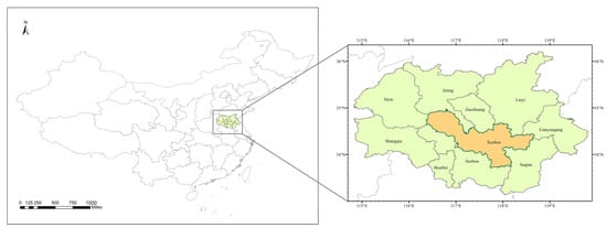
Figure 1.
The study area (116°22′–118°40′ E, 33°43′–34°58′ N).
2.2. Data source and Description
2.2.1. Reanalysis Data—MERRA-2
Global Modeling and Assimilation Office (GMAO) of NASA has produced Modern-Era Retrospective analysis for Research and Applications version 2 (MERRA-2), which is the latest version of global atmospheric reanalysis for the satellite era. It utilizes GEOS5.12.4 to generate a long time series of reanalysis datasets. MERRA-2 is committed to providing a regular and uniform set of meteorological data covering the world, and it provides up to 21 types of product data.
This paper chooses to use the “MERRA-2 tavg1_2d_aer_Nx in MERRA-2: 2 d, 1–Hourly, Time-averaged, Single-Level, Assimilation, Aerosol Diagnostics V5.12.4“ dataset [42]. The data collection in MERRA-2 consists of two-dimensional data that is averaged over hourly intervals. This collection consists of assimilated aerosol diagnostics, including various types, and in this paper, the total extinction (and scattering) AOD at 550 nm is selected for the experiment. Its spatial resolution is 0.5° × 0.625°, its temporal resolution is 1 h, and its data format is NetCDF4.
2.2.2. Ground Monitoring Data
The ground monitoring data used in this paper is the hourly pollutant concentration data released by the China National Environmental Monitoring Station, which is collected from the National Real-Time Release Platform for Urban Air Quality [43]. Ground measurement data includes AQI, PM2.5, and PM10. After regional screening, 65 sites can be used in this study and the distribution of sites is shown in Figure 2. Furthermore, to guarantee data accuracy, this study has performed elimination of invalid values, which are displayed as null, and aberrant values exceeding 1000 or below 0, resulting from instrument calibration issues.
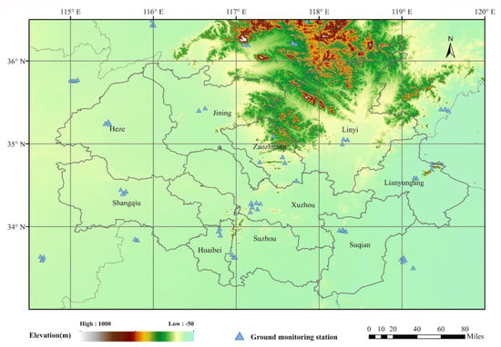
Figure 2.
Spatial distributions of ground monitoring stations (blue triangles) in 2020 across the HHEZ, where the background is the surface elevation (m).
Since other data used in this study are all in United Technology Corporation (UTC), while the ground monitoring data are in local time (LT), a step of time conversion is required before using these data. The specific conversion formula in this study is shown in Equation (1).
2.2.3. Wind Data
The meteorological data such as wind speed and wind direction used in this study are ERA5 from European Center for Medium Weather Forecasting (ECMWF), Shinfield Park, Reading, United Kingdom [44]. ERA5, the fifth-generation ECMWF reanalysis for global climate and weather, is a comprehensive and consistent global dataset that covers a wide range of variables. The two parameters used in this paper are 10 m u-component of wind and 10 m v-component of wind. The 10 m u-component of wind is the horizontal component of the wind at 10 m height in the eastward direction. Similarly, the 10 m v-component of wind refers to the northward component of wind in the horizontal direction.
The details of the aforementioned variables are shown in Table 1.

Table 1.
Description of data used in the study.
2.3. Research Methodology
This study used MERRA-2 AOD data at 550 nm and combined it with ground monitoring data to determine the pollution threshold. The region where the polluted air mass is located can be obtained by screening with this threshold value. In this paper, a “Time-Longitude-Latitude” three-dimensional pollution curve is established with time as the independent variable and longitude and latitude as the dependent variable. Genetic algorithm was used to optimize the curve fitting. Finally, the maximum possible pollution transmission route within the experimental area can be reconstructed. The overall procedure of the pollution route reconstruction is shown in Figure 3.
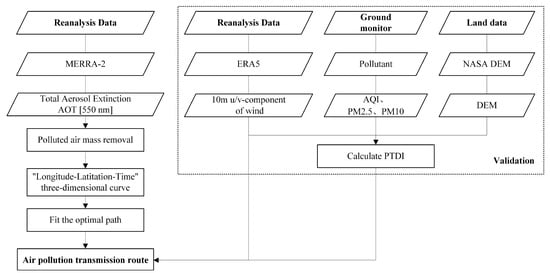
Figure 3.
The flowchart of the pollution transmission route reconstruction method in this study. DEM is the digital elevation model and PTDI stands for the Pollution Transfer Diffusion Index.
2.3.1. AOD Pollution Threshold Screening
To investigate the relationship between AOD and air pollution, this study analyzed the corresponding pollutant concentration data and AOD values in the study area on 12 January 2020. Hourly pollutant concentration data from 65 air quality ground monitoring stations were utilized. The results revealed that when the AOD is greater than 1.2, 90.53% of the hourly PM2.5 concentration exceeded 75 , as shown in Figure 4, indicating a polluted air quality level. Furthermore, the study aimed to determine the presence of a transmission route, which requires further conditional judgment and fulfillment of the following two conditions: firstly, the polluted AOD remote sensing image should demonstrate a continuous shape; secondly, the pollution range should exhibit a consistent direction of movement. In order to achieve accurate judgment of these two conditions, after repeated experiments, this paper selected an AOD value of 1.2 as the threshold for screening polluted air masses for the pollution process on 12 January 2020. In addition, the experiment also removed the dirty values of the data to avoid large errors caused by outliers of AOD products and scattered grids.
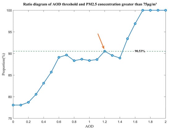
Figure 4.
The relationship between AOD and PM2.5. The point indicated by the arrow is the critical value we have chosen, and the green line indicates that when the AOD is greater than 1.2, 90.53% of the hourly PM2.5 concentration exceeds 75 .
2.3.2. Construction of “Time-Longitude-Latitude” Three-Dimensional Pollution Curve
This paper analyzes the pollution transport process using total extinction (and scattering) aerosol optical depth at 550 nm data of MERRA-2. In order to unify and standardize the spatiotemporal multivariate data of multidimensional information such as time, AOD concentration values, and geographic coordinates, this paper restructured the MERRA-2 data. Based on the AOD, this study establishes a “Time-Longitude-Latitude” three-dimensional pollution curve with time as the independent variable and longitude and latitude as the dependent variables. It simplifies the expression of abstract pollution processes for subsequent calculations and analyses.
2.3.3. Optimal Path Fitting Based on Genetic Algorithm
Genetic algorithm (GA) was originally proposed by J. H. Holland in the United States in 1975 in his monograph “Adaptation in nature and artificial systems” [45]. It is an optimal solution search algorithm that simulates natural genetic theory and biological evolution theory. GA simulates the phenomena of reproduction, crossover, and gene mutation in natural genetic processes, retaining a set of solutions in each iteration process and selecting the optimal individuals from the solution group according to indicators. Then, genetic operators are used to combine these individuals to generate a new generation of solution groups, and the above process is repeated until the convergence goal is met to obtain the optimal solution.
In order to obtain the maximum possible pollution transmission route within the study area, this paper uses genetic algorithm to perform optimal curve fitting on the “Time-Longitude-Latitude” three-dimensional pollution curve. The basic idea is to know a set of filtered polluted air mass data and then set a reference expression based on prior knowledge that can simulate the pollution transfer curve. Under certain criteria, the simulated three-dimensional pollution curve is most consistent with the filtered pollution data. The technical route is shown in Figure 5.
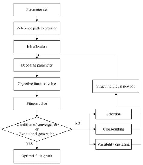
Figure 5.
Technical route of genetic algorithm.
In the parameter setting process of GA, this study specifically adds the step of setting reference path expressions based on prior knowledge to prevent significant errors in the path iteration and fitting processes [46]. This step ensures the correctness and accuracy of path fitting to the greatest extent. In the process of parameter optimization in GA, the most crucial step is to select the appropriate fitness function, which is the basis for judging the quality of each solution, that is, the formulation of the objective function. The objective function used in this article is as follows:
where is the corresponding latitude on the simulated pollution transfer curve, represents the center latitude of each grid of the actual filtered polluted air masses, is the actual distance length represented by each grid at that latitude, and R is the difference between the two, which reflects the error between the simulated curve and the actual transmission path of the polluted air masses. The objective function uses absolute values to prevent mutual cancellation of positive and negative errors.
2.3.4. Calculation of Pollution Transfer Diffusion Index
To verify the correctness of the fitting path, this paper proposes the Pollution Transfer Diffusion Index (PTDI), which is calculated by overlaying the pollutant concentration of ground monitoring stations, wind speed, terrain, and other influencing factors. The biggest advantage of PTDI is that it does not require the specific calculation of pollutant emissions in the target area, but directly uses the pollutant concentration values from ground monitoring stations for calculation. The specific equations are as follows:
where C is the concentration of pollutants, in units of , obtained from monitoring data from the China National Environmental Monitoring Station; K is the diffusion coefficient, in units of , it reflects the effect of wind speed on the transport of pollutants; u is the wind speed, in ; h is the atmospheric stability parameter. This formula uses the Pasquill-Gifford stability classification method to divide the atmosphere into six stability levels, A-F, with each stability level corresponding to a range of h values; H is the air quality stability parameter. The index can be used to describe the transport, diffusion, and concentration distribution of pollutants in the atmosphere. It is a comprehensive indicator that reflects the changes in air pollutants over time and distance.
3. Results and Discussion
3.1. Reconstruction of Pollution Transmission Route
This paper used total extinction (and scattering) aerosol optical depth at 550 nm data of reanalysis data MERRA-2 as the main basis for hourly AOD concentration values. According to the analysis of AOD values and transmission route judgment criteria, a serious air pollution event occurred on 12 January 2020 from 9:00 to 24:00 (UTC) in the central and southern regions of the HHEZ. It has an obvious pollution transmission process. Figure 6a–i shows the transmission process of this pollution. It can be concluded that the transmission process of this pollution primarily occurred from 9:00 to 24:00. This process originated in Zhoukou City, Henan Province and continued to spread in an east-north direction. It passed through the northern part of Fuyang, the southern part of Shangqiu, the northern part of Huaibei, and the central part of Suzhou. At 16:00 (UTC), the pollution center arrived in the southwestern part of Xuzhou and began to transmit towards the southeast due to factors such as wind and terrain. Subsequently, the pollution centers stayed in the central part of Suzhou and the southeastern part of Xuzhou, spanning across the central part of Suqian. It arrived in the northern part of Huai’an at 22:00 (UTC). Then, it began to circulate westward due to the influence of wind direction and pollution emissions from areas such as Suzhou and Huaibei. Figure 7 shows the specific transmission route and corresponding time nodes of this pollution process. It is reconstructed by combining the optimal “Time-Longitude-Latitude” three-dimensional pollution curve fitted based on genetic algorithm.
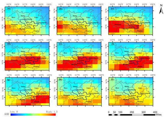
Figure 6.
The pollution transmission process demonstrated with AOD of MERRA-2 on 12 January 2020 in the HHEZ. (a–i) display images of 9:00, 10:00, 12:00, 14:00, 16:00, 18:00, 20:00, 22:00 and 23:00 insequence.
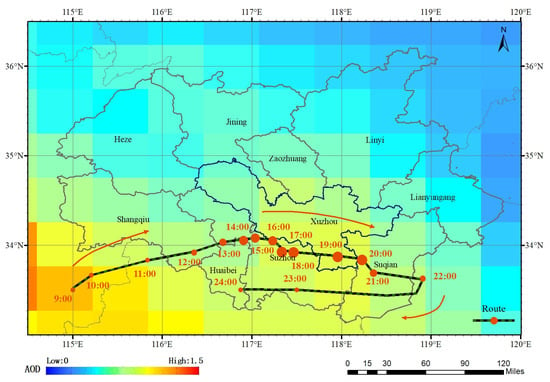
Figure 7.
The specific transmission route and corresponding time nodes of the pollution process on 12 January 2020 in the HHEZ.
On a larger scale, this pollution is not entirely caused by the local pollution in these four provinces of Jiangsu, Shandong, Anhui, and Henan. The long-distance transmission of pollution from external areas has further exacerbated the severity of this pollution, with a large portion of the pollution sources appearing to come from the border between Shaanxi and Gansu provinces. Specifically, it mainly came from the northern part of Baoji City and the northwest part of Xianyang City in Shaanxi Province. Figure 8a–i clearly illustrates this process. The polluted air mass moved eastward from the central region of Shaanxi Province and began to affect the westernmost city of the HHEZ at 9:00(UTC) on 12 January 2020.
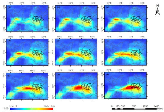
Figure 8.
The pollution transmission process demonstrated with AOD of MERRA-2 on 12 January 2020 on a larger scale. (a–i) display images of 2:00, 4:00, 5:00, 6:00, 7:00, 8:00, 9:00, 10:00 and 12:00 insequence.
3.2. Validation and Analysis of Pollution Transmission Route
3.2.1. Comparison and Verification with Pollution Index
PTDI was calculated using data such as pollutant concentration of ground monitoring stations (Figure 9) and wind speed (Figure 10). PTDI to generate a pollution index. The contour map is drawn, as shown in Figure 11. Then, the paper conducts a gradient change analysis (Figure 12) to assist in determining the pollution transmission situation on that day. Based on the above analysis, it can be determined that the severe air pollution event in Xuzhou City on 12 January 2020 was not caused by local emissions. It was mainly caused by external transmission. The pollution source came from the southwest direction. This result is basically consistent with the experimental results of the pollution transmission route reconstruction mentioned in this paper.
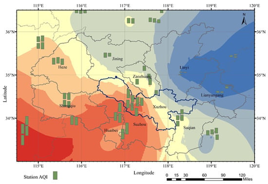
Figure 9.
AQI distribution of ground monitoring stations on 12 January 2020 in the HHEZ.
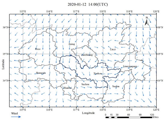
Figure 10.
Wind speed and direction at 10 m at 14:00 on 12 January 2020 in the HHEZ.
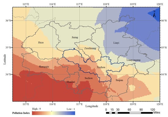
Figure 11.
Distribution of pollution index on 12 January 2020 in the HHEZ.
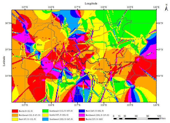
Figure 12.
The results of the gradient change analysis of the pollution index.
3.2.2. Comparison Analysis with Wind Field Data
In addition, this paper also used wind speed and direction data at 10 m from 7:00 to 24:00 (UTC) on 12 January 2020 from ERA5 to perform mean simulation, as shown in Figure 13. On that day, the airflow in the heavily polluted central and southern regions of the HHEZ mainly showed a trend of moving from west to east, which led to the continuous transportation of pollutants from west to east. Specifically, there were many local circulations in the wind field on that day. Among them, there was a significant change in wind direction at the junction of Xuzhou, Suqian, and Suzhou. This is highly consistent with the pollution transmission route results mentioned above, as analyzed from the AOD data of MERRA-2.
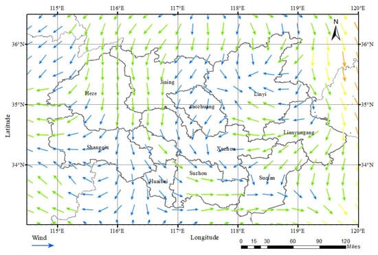
Figure 13.
Average modelled wind speed and direction at 10 m on 12 January 2020 in the HHEZ. The direction of the arrow represents the wind direction, and the color of the arrow represents the size of the wind speed. The bluer the color, the lower the wind speed, and the redder the color, the higher the wind speed.
3.2.3. Comparison Analysis with Other Trajectory Models
A Hybrid Single Particle Lagrangian Integrated Trajectory Model (HYSPLIT) is one of the most widely used transport and diffusion models in the field of atmospheric science [47,48]. In order to more intuitively show the prediction effect of the fit, we chose the backward trajectory analysis in the HYSPLIT. It was used to simulate the trajectory of atmospheric air masses at different altitudes in the area during this period, thereby establishing the origin of the air masses and establishing a source receptor relationship. We used the cluster analysis method to integrate trajectories and simulated the possible source directions and composition proportions of this pollution transmission. The results showed that they have a high similarity, as shown in Figure 14. This figure shows the backward trajectory clustering results of Global Data Assimilation System (GDAS) meteorological data at a height of 1000 m. We can see in the figure that the blue trajectory accounts for 32%. It started at the border between Shaanxi and Gansu provinces, passed through Henan Province, and finally entered HHEZ. It is the largest proportion of the possible source direction for this pollution transmission, which is highly consistent with the reconstruction path analysis in Section 3.1 above.
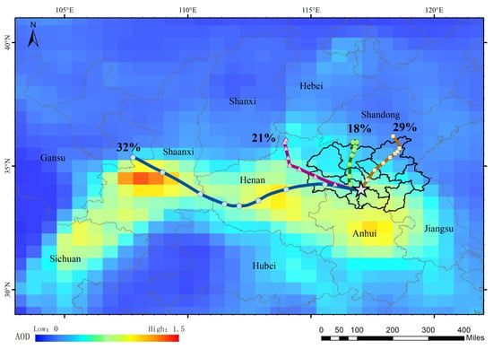
Figure 14.
Backward trajectory clustering results of HYSPLIT. The five−pointed star represents the polluted areas in the HHEZ and the four color lines represent possible sources of pollution.
3.3. Application of This Method in Other Regions
To verify the universality of this method and ensure its generalizability, another region in China with distinct characteristics was chosen for experimentation in this study. The experimental area is mainly composed of an urban cluster of the Beijing-Tianjin-Hebei Urban Agglomeration, including the Bohai Sea located on its east side. This experiment’s selected air pollution event occurred on 1 June 2020.
Figure 15a–l shows the transmission process of the pollution. It can be determined that the transmission process of this pollution mainly occurred from 8:30 (UTC) on June 1st to 00:30 (UTC) the next day. The pollution originated at the junction of Baoding and Beijing. Specifically, it is in the northeast of Baoding City, Hebei Province, and continues to spread eastward, passing through Fangshan District and Daxing District of Beijing, and then the pollution center shifted slightly southward and returned to Langfang, Hebei Province. At 12:30 (UTC), the pollution center arrived in Tianjin, passed through Wuqing District, Beichen District, Dongli District, and Jinnan District once, and reached Binhai New District at 14:30 (UTC). Subsequently, the polluted air masses arrived over the Bohai Sea, and under the influence of wind and other factors, pollutants were transported and diffused deep into the Bohai Sea, ultimately dissipating at sea. Figure 16 shows the specific transmission route and corresponding time nodes of the pollution process reconstructed by combining the optimal “Time-Longitude-Latitude “ three-dimensional pollution curve fitted based on genetic algorithm.
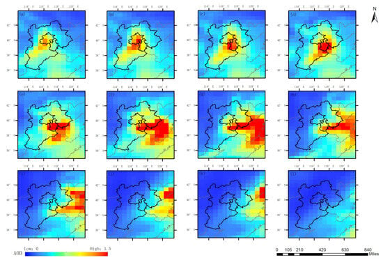
Figure 15.
The pollution transmission process demonstrated with AOD of MERRA-2 on 1 June 2020 in the Beijing-Tianjin-Hebei Urban Agglomeration. (a–l) display the images of 9:00, 10:00, 11:00, 12:00, 14:00, 18:00, 20:00, 22:00 on June 1, and 0:00, 2:00, 4:00 on June 2, in turn.
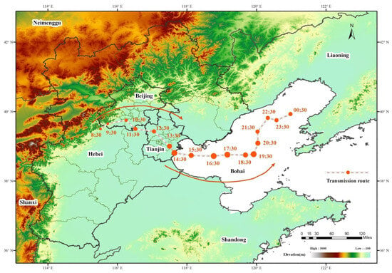
Figure 16.
The specific transmission route and corresponding time nodes of the pollution process on 1 June 2020 in the Beijing-Tianjin-Hebei Urban Agglomeration. The arrows represent the direction of pollution transport.
4. Conclusions
This paper introduced a method for reconstructing pollution transmission routes based on the “Time-Longitude-Latitude” three-dimensional pollution curve, combining the AOD dataset of reanalysis data MERRA-2, hourly pollutant concentration data of ground monitoring stations, and meteorological data of reanalysis dataset ERA5. It is worth mentioning that this article innovatively combines the concept of three-dimensional curves and genetic algorithms to unify and standardize the spatiotemporal multivariate data of atmospheric pollution from satellite remote sensing. This article used this method to restore and reconstruct two instances of air pollution transmission processes that occurred in two representative regions in China in 2020. By applying this method, we successfully identified the sources, input paths, and affected time periods of these severe air pollution events. The successful application of this method can enable the environmental protection department to accurately reconstruct the air pollution transmission route in the later stage, accurately identify the imported air pollution source, and quickly find the air pollution transmission entrance. Thanks to the support of these data and technologies, policy-making departments can be more targeted to propose scientific and efficient imported air pollution prevention and control strategies. At the same time, it is also possible to trace pollution responsibilities more effectively and achieve regional joint governance. As such, urban air quality would be improved more scientifically and efficiently.
Author Contributions
Conceptualization, X.L. and Y.X.; methodology, X.L. and Y.X.; software, X.L. and B.H.; validation, X.L. and B.H.; formal analysis, X.L.; investigation, X.L. and B.H.; resources, Y.X.; data curation, X.L. and X.J.; writing—original draft preparation, X.L.; writing—review and editing, X.L., B.H. and Y.X.; visualization, X.L. and B.H.; supervision, S.W. and X.W.; project administration, Y.X.; funding acquisition, Y.X. All authors have read and agreed to the published version of the manuscript.
Funding
This work was jointly supported by the National Natural Science Foundation of China (NSFC) under Grant No. 42275147.
Institutional Review Board Statement
Not applicable.
Informed Consent Statement
Not applicable.
Data Availability Statement
The datasets generated during and/or analyzed during the current study are available from the corresponding author on reasonable request.
Acknowledgments
We thank the contributors and supporters of the datasets used in the study, including MERRA-2 AOD product, ERA5 hourly data, and ground monitoring data from the China National Environmental Monitoring Station. And we gratefully acknowledge the NOAA Air Resources Laboratory (ARL) for the provision of the HYSPLIT transport and dispersion model and/or READY website (https://www.ready.noaa.gov/ accessed on 3 September 2023) used in this publication.
Conflicts of Interest
The authors declare no conflict of interest.
References
- Han, L.; Zhou, W.; Li, W.; Li, L. Impact of urbanization level on urban air quality: A case of fine particles (PM2.5) in Chinese cities. Environ. Pollut. 2014, 194, 163–170. [Google Scholar] [CrossRef] [PubMed]
- Hao, Y.; Liu, Y. The influential factors of urban PM2.5 concentrations in China: A spatial econometric analysis. J. Clean. Prod. 2016, 112, 1443–1453. [Google Scholar] [CrossRef]
- Chan, C.K.; Yao, X. Air pollution in mega cities in China. Atmos. Environ. 2008, 42, 1–42. [Google Scholar] [CrossRef]
- Shi, M.; Wu, H.; Zhang, S.; Li, H.; Yang, T.; Liu, W.; Liu, H. Weekly cycle of magnetic characteristics of the daily PM2.5 and PM2.5–10 in Beijing, China. Atmos. Environ. 2014, 98, 357–367. [Google Scholar] [CrossRef]
- Zhang, L.; Zhao, N.; Zhang, W.; Wilson, J.P. Changes in long-term PM2.5 pollution in the urban and suburban areas of China’s three largest urban agglomerations from 2000 to 2020. Remote Sens. 2022, 14, 1716. [Google Scholar] [CrossRef]
- Wang, H.; Xu, J.; Zhang, M.; Yang, Y.; Shen, X.; Wang, Y.; Chen, D.; Guo, J. A study of the meteorological causes of a prolonged and severe haze episode in January 2013 over central-eastern China. Atmos. Environ. 2014, 98, 146–157. [Google Scholar] [CrossRef]
- Kozáková, J.; Pokorná, P.; Vodička, P.; Ondráčková, L.; Ondráček, J.; Křůmal, K.; Mikuška, P.; Hovorka, J.; Moravec, P.; Schwarz, J. The influence of local emissions and regional air pollution transport on a European air pollution hot spot. Environ. Sci. Pollut. R. 2019, 26, 1675–1692. [Google Scholar] [CrossRef] [PubMed]
- Sorte, S.; Arunachalam, S.; Naess, B.; Seppanen, C.; Rodrigues, V.; Valencia, A.; Borrego, C.; Monteiro, A. Assessment of source contribution to air quality in an urban area close to a harbor: Case-study in Porto, Portugal. Sci. Total Environ. 2019, 662, 347–360. [Google Scholar] [CrossRef]
- Wang, Y.; Li, Y.; Qiao, Z.; Lu, Y. Inter-city air pollutant transport in the Beijing-Tianjin-Hebei urban agglomeration: Comparison between the winters of 2012 and 2016. J. Environ. Manag. 2019, 250, 109520. [Google Scholar] [CrossRef]
- Bai, Y.; Zhao, T.; Hu, W.; Zhou, Y.; Xiong, J.; Wang, Y.; Liu, L.; Shen, L.; Kong, S.; Meng, K.; et al. Meteorological mechanism of regional PM2.5 transport building a receptor region for heavy air pollution over central China. Sci. Total Environ. 2022, 808, 151951. [Google Scholar] [CrossRef]
- Tessum, M.W.; Anenberg, S.C.; Chafe, Z.A.; Henze, D.K.; Kleiman, G.; Kheirbek, I.; Marshall, J.D.; Tessum, C.W. Sources of ambient PM2.5 exposure in 96 global cities. Atmos. Environ. 2022, 286, 119234. [Google Scholar] [CrossRef]
- Macpherson, A.J.; Simon, H.; Langdon, R.; Misenheimer, D. A mixed integer programming model for National Ambient Air Quality Standards (NAAQS) attainment strategy analysis. Environ. Modell. Softw. 2017, 91, 13–27. [Google Scholar] [CrossRef]
- Wu, D.; Fung, J.C.H.; Yao, T.; Lau, A.K.H. A study of control policy in the Pearl River Delta region by using the particulate matter source apportionment method. Atmos. Environ. 2013, 76, 147–161. [Google Scholar] [CrossRef]
- Ji, Y.; Qin, X.; Wang, B.; Xu, J.; Shen, J.; Chen, J.; Huang, K.; Deng, C.; Yan, R.; Xu, K.; et al. Counteractive effects of regional transport and emission control on the formation of fine particles: A case study during the Hangzhou G20 summit. Atmos. Chem. Phys. 2018, 18, 13581–13600. [Google Scholar] [CrossRef]
- Grennfelt, P.; Hov, O. Regional air pollution at a turning point. Ambio 2005, 34, 2–10. [Google Scholar] [CrossRef] [PubMed]
- Holnicki, P.; Kałuszko, A.; Nahorski, Z.; Tainio, M. Intra-urban variability of the intake fraction from multiple emission sources. Atmos. Pollut. Res. 2018, 9, 1184–1193. [Google Scholar] [CrossRef] [PubMed]
- Bohnenstengel, S.I.; Belcher, S.E.; Aiken, A.; Allan, J.D.; Allen, G.; Bacak, A.; Bannan, T.J.; Barlow, J.F.; Beddows, D.; Bloss, W.J.; et al. Meteorology, air quality, and health in London the clearflo project. Bull. Am. Meteorol. Soc. 2015, 96, 779–804. [Google Scholar] [CrossRef]
- Liu, M.; Lei, Y.; Wang, X.; Xue, W.; Zhang, W.; Jiang, H.; Wang, J.; Bi, J. Source contributions to PM2.5-related mortality and costs: Evidence for emission allocation and compensation strategies in China. Environ. Sci. Technol. 2023, 57, 4720–4731. [Google Scholar] [CrossRef]
- Park, S.; Lee, J.; Im, J.; Song, C.; Choi, M.; Kim, J.; Lee, S.; Park, R.; Kim, S.; Yoon, J.; et al. Estimation of spatially continuous daytime particulate matter concentrations under all sky conditions through the synergistic use of satellite-based AOD and numerical models. Sci. Total Environ. 2020, 713, 136516. [Google Scholar] [CrossRef]
- Hoff, R.M.; Christopher, S.A. Remote sensing of particulate pollution from space: Have we reached the promised land? J. Air Waste Manag. 2009, 59, 645–675. [Google Scholar] [CrossRef]
- Martin, R.V. Satellite remote sensing of surface air quality. Atmos. Environ. 2008, 42, 7823–7843. [Google Scholar] [CrossRef]
- Lin, C.; Li, Y.; Yuan, Z.; Lau, A.K.H.; Li, C.; Fung, J.C.H. Using satellite remote sensing data to estimate the high-resolution distribution of ground-level PM2.5. Remote Sens. Environ. 2015, 156, 117–128. [Google Scholar] [CrossRef]
- Zhang, L.; Wilson, J.P.; Macdonald, B.; Zhang, W.; Yu, T. The changing PM2.5 dynamics of global megacities based on long-term remotely sensed observations. Environ. Int. 2020, 142, 105862. [Google Scholar] [CrossRef] [PubMed]
- Zhang, L.; Wilson, J.P.; Zhao, N.; Zhang, W.; Wu, Y. The dynamics of cardiovascular and respiratory deaths attributed to long-term PM2.5 exposures in global megacities. Sci. Total Environ. 2022, 842, 156951. [Google Scholar] [CrossRef] [PubMed]
- Lee, H.J.; Liu, Y.; Coull, B.A.; Schwartz, J.; Koutrakis, P. A novel calibration approach of MODIS AOD data to predict PM2.5 Concentrations. Atmos. Chem. Phys. 2011, 11, 7991–8002. [Google Scholar] [CrossRef]
- Sun, Y.; Xue, Y.; Jiang, X.; Jin, C.; Wu, S.; Zhou, X. Estimation of the PM2.5 and PM10 mass concentration over land from FY-4A aerosol optical depth data. Remote Sens. 2021, 13, 4276. [Google Scholar] [CrossRef]
- Chudnovsky, A.A.; Koutrakis, P.; Kloog, I.; Melly, S.; Nordio, F.; Lyapustin, A.; Wang, Y.; Schwartz, J. Fine particulate matter predictions using high resolution aerosol optical depth (AOD) retrievals. Atmos. Environ. 2014, 89, 189–198. [Google Scholar] [CrossRef]
- Wang, J.; Christopher, S.A. Intercomparison between satellite-derived aerosol optical thickness and PM2.5 mass: Implications for air quality studies. Geophys. Res. Lett. 2003, 30. [Google Scholar] [CrossRef]
- Liu, Y.; Park, R.J.; Jacob, D.J.; Li, Q.; Kilaru, V.; Sarnat, J.A. Mapping annual mean ground-level PM2.5 concentrations using multiangle imaging spectroradiometer aerosol optical thickness over the contiguous united states. J. Geophys. Res. Atmos. 2004, 109. [Google Scholar] [CrossRef]
- Odén, S. Acidification of Air and Precipitation and Its Consequences on the Natural Environment; Swedish State Natural Science Research Council: Stockholm, Sweden, 1968. [Google Scholar]
- Tian, J.; Fang, C.; Qiu, J.; Wang, J. Analysis of pollution characteristics and influencing factors of main pollutants in the atmosphere of Shenyang city. Atmosphere 2020, 11, 766. [Google Scholar] [CrossRef]
- Jorba, O.; Perez, C.; Rocadenbosch, F.; Baldasano, J.M. Cluster analysis of 4-day back trajectories arriving in the Barcelona area, Spain, from 1997 to 2002. J. Appl. Meteorol. 2004, 43, 887–901. [Google Scholar] [CrossRef]
- Escudero, M.; Stein, A.; Draxler, R.R.; Querol, X.; Alastuey, A.; Castillo, S.; Avila, A. Determination of the contribution of northern Africa dust source areas to pm10 concentrations over the central Iberian peninsula using the hybrid single-particle Lagrangian integrated trajectory model (HYSPLIT) model. J. Geophys. Res. 2006, 111. [Google Scholar] [CrossRef]
- Ara Begum, B.; Kim, E.; Jeong, C.; Lee, D.; Hopke, P.K. Evaluation of the potential source contribution function using the 2002 Quebec forest fire episode. Atmos. Environ. 2005, 39, 3719–3724. [Google Scholar] [CrossRef]
- Stohl, A.; Forster, C.; Frank, A.; Seibert, P.; Wotawa, G. Technical note: The Lagrangian particle dispersion model FLEXPART version 6.2. Atmos. Chem. Phys. 2005, 5, 2461–2474. [Google Scholar] [CrossRef]
- Xu, R.; Zhang, H.; Yang, X.; Cheng, S.; Zhang, T.; Jiang, Q. Concentration characteristics of PM2.5 and the causes of heavy air pollution events in Beijing during autumn and winter. Huan Jing Ke Xue 2019, 40, 3405–3414. [Google Scholar] [CrossRef] [PubMed]
- Ma, J.; Shen, J.; Wang, P.; Zhu, S.; Wang, Y.; Wang, P.; Wang, G.; Chen, J.; Zhang, H. Modeled changes in source contributions of particulate matter during the covid-19 pandemic in the Yangtze River Delta, China. Atmos. Chem. Phys. 2021, 21, 7343–7355. [Google Scholar] [CrossRef]
- Livingstone, P.L.; Magliano, K.; Guerer, K.; Allen, P.D.; Zhang, K.M.; Ying, Q.; Jackson, B.S.; Kaduwela, A.; Kleeman, M.; Woodhouse, L.F.; et al. Simulating pm concentration during a winter episode in a subtropical valley: Sensitivity simulations and evaluation methods. Atmos. Environ. 2009, 43, 5971–5977. [Google Scholar] [CrossRef]
- Xue, W.; Wang, J.; Yang, J.; Lei, Y.; Wang, Y.; Chen, X. Domestic and Foreign Research Progress of Air Quality Model. Environ. Sustain. Dev. 2013, 38, 14–20. (In Chinese) [Google Scholar]
- Eun Kim, S. Nonlinear estimation for PM2.5 transmission effects in Jefferson Co., Texas. Environmetrics 2004, 15, 369–380. [Google Scholar] [CrossRef]
- Wang, Y.; Du, H.; Xu, Y.; Lu, D.; Wang, X.; Guo, Z. Temporal and spatial variation relationship and influence factors on surface urban heat island and ozone pollution in the Yangtze River Delta, China. Sci. Total Environ. 2018, 631–632, 921–933. [Google Scholar] [CrossRef]
- Global Modeling and Assimilation Office (GMAO). MERRA-2 tavg1_2d_aer_Nx: 2d,1-Hourly, Time-Averaged, Single-Level, Assimilation, Aerosol Diagnostics V5.12.4; Goddard Earth Sciences Data and Information Services Center (GES DISC): Greenbelt, MD, USA, 2015. [Google Scholar] [CrossRef]
- China National Environmental Monitoring Centre. National Environmental Air Quality Monitoring Network. 8 November 2017. Available online: http://www.cnemc.cn/zzjj/jcwl/dqjcwl/201711/t20171108_645109.shtml (accessed on 10 November 2022).
- Radu, R.C.; Rozum, I.; Schepers, D.; Simmons, A.; Soci, C.; Dee, D.; Thépaut, J.-N. ERA5 Hourly Data on Single Levels from 1959 to Present; Copernicus Climate Change Service (C3S) Climate Data Store (CDS): Reading, UK, 2018. [Google Scholar] [CrossRef]
- Holland, J.H. Adaptation in Natural and Artificial Systems: An Introductory Analysis with Applications to Biology, Control, and Artificial Intelligence; MIT Press: Cambridge, MA, USA, 1992. [Google Scholar]
- Marinakis, Y.; Marinaki, M. A hybrid genetic-particle swarm optimization algorithm for the vehicle routing problem. Expert Syst. Appl. 2010, 37, 1446–1455. [Google Scholar] [CrossRef]
- Stein, A.; Draxler, R.; Rolph, G.; Stunder, B.; Cohen, M.; Ngan, F. NOAA’s HYSPLIT Atmospheric Transport and Dispersion Modeling System. Bull. Am. Meteorol. Soc. 2015, 96, 2059–2077. Available online: https://journals.ametsoc.org/view/journals/bams/96/12/bams-d-14-00110.1.xml (accessed on 3 September 2023). [CrossRef]
- Rolph, G.; Stein, A.; Stunder, B. Real-time environmental applications and display system: Ready. Environ. Modell. Softw. 2017, 95, 210–228. [Google Scholar] [CrossRef]
Disclaimer/Publisher’s Note: The statements, opinions and data contained in all publications are solely those of the individual author(s) and contributor(s) and not of MDPI and/or the editor(s). MDPI and/or the editor(s) disclaim responsibility for any injury to people or property resulting from any ideas, methods, instructions or products referred to in the content. |
© 2023 by the authors. Licensee MDPI, Basel, Switzerland. This article is an open access article distributed under the terms and conditions of the Creative Commons Attribution (CC BY) license (https://creativecommons.org/licenses/by/4.0/).