Application of Machine Learning Techniques to Improve Multi-Radar Mosaic Precipitation Estimates in Shanghai

Abstract

In this study, we applied an explainable machine learning technique based on the LightGBM method, a category of gradient boosting decision tree algorithm, to conduct a quantitative radar precipitation estimation and move to understand the underlying reasons for excellent estimations. By introducing 3D grid radar reflectivity data into the LightGBM algorithm, we constructed three LightGBM models, including 2D and 3D LightGBM models. Ten groups of experiments were carried out to compare the performances of the LightGBM models with traditional Z–R relationship methods. To further assess the performances of the LightGBM models, rainfall events with 11,483 total samples during August-September of 2022 were used for statistical analysis, and two heavy rainfall events were specifically chosen for the spatial distribution evaluation. The results from both the statistical analysis and spatial distribution demonstrate that the performance of the LightGBM 3D model with nine points is the best method for quantitative precipitation estimation in this study. Through analyzing the explainability of the LightGBM models from Shapley additive explanations (SHAP) regression values, it can be inferred that the superior performance of the LightGBM 3D model is mainly attributed to its consideration of the rain gauge station attributes, diurnal variation characteristics, and the influence of spatial offset.

1. Introduction

Quantitative precipitation estimation (QPE), as the basis of quantitative precipitation forecasting and short-term and imminent warnings of heavy precipitation, plays an important supporting role in agriculture, flash flood warning operations, streamflow predictions, and water resource management [1,2,3,4]. Given the good performance of radar data in spatial distributions, using radar data to produce a QPE is also conducive to solving the problem that precipitation data are only available at limited sites [5]. For instance, blending radar precipitation estimates that have better spatial and temporal coverage with accurate rain gauge data can produce a gridded precipitation dataset over regions of insufficient gauge density [5,6,7]. The multi-radar system can provide observational data for producing rapid update quantitative precipitation estimations over special terrain surfaces, such as lakes and high-altitude mountainous areas, with high spatial and temporal resolution [1].

Radar reflectivity reflects the content of hydrometeors (such as water droplets or ice particles) in the atmosphere, which correlates well with the rainfall rate [8]. Therefore, the radar reflectivity factor is often used as an input variable to estimate the precipitation rate [9,10]. An operational radar QPE method, the Z–R relationship [11], was proposed by the assumed nonlinear relationship between the radar reflectivity factor (Z) and rainfall rate (R). However, the Z–R relationship is dependent on the raindrop size distribution, which can vary across different precipitation types and regions [12,13], and this uncertainty is one of the primary error sources of radar QPEs [1,14]. Fixed Z–R relationship approaches can be problematic in cases where the relationships vary spatially or temporally throughout a region [15]. For example, the radar precipitation fields obtained from the currently used Marshall–Palmer Z–R relationship show a systematic underestimation [15].

It is important to consider these variations when using the Z–R relationship to estimate rainfall rates since the localized differences can affect its accuracy. Many studies take these factors into account to develop region-specific Z–R relationships for more accurate precipitation estimations. In order to improve the radar QPE, a real-time adjustment to the radar reflectivity–rainfall rates (Z–R) relationship scheme with inverse distance weighting interpolation was developed by Wang et al. (2012) [16]. Alfieri et al. (2010) suggested that the Z–R relationship varies over time [17], and thus they proposed a time-dependent (dynamic) Z–R relationship. This Z–R relationship in a short period should be redetermined by the observed precipitation and radar reflectivity [17]. Shao et al. (2021) reconstructed a local Z–R relationship using a genetic optimization algorithm to minimize the errors from different rainfall patterns and climate zones [7]. Wu et al. (2018) proposed a dynamical Z–R relationship to improve the precipitation estimation over the Yangtze River based on radar echo-top height classification [13]. However, these optimized Z–R relationship methods still struggle to capture the features of rainfall intensity or spatial distribution accurately.

The development of artificial intelligence technology also provides new technical support for QPEs. Concurrent research applying the techniques from artificial intelligence literature has shown that quantitative precipitation can be estimated using machine learning methods. For example, Kuang et al. (2016) improved rainfall estimation accuracy by proposing a random forest and linear chain conditional spatiotemporal model [18]. Wolfensberger et al. (2021) proposed a QPE model by training a random forest regression that can significantly reduce the bias of precipitation intensities but overestimate weak precipitation [19]. Based on support vector machine (SVM) algorithms [20], Sehad et al. (2017) improved the rainfall estimation over the north of Algeria using Meteosat Second Generation [21]. Although artificial intelligence methods have shown some advantages in radar precipitation estimations, there are still lots of challenges in explaining the ability of artificial intelligence technology.

In recent research, the application of explainable artificial intelligence techniques has shown great promise in evaluating how various machine learning techniques make predictions or estimations [22,23,24,25,26]. Silva et al. (2022) used XGBoost classification trees [27] and Shapley additive explanations (SHAP) analysis to explore errors in the prediction of lightning occurrence [25]. Stirnberg et al. (2021) applied the SHAP regression values to quantify the importance of various meteorological drivers on particulate matter concentrations [28].

The radar–precipitation estimation dataset in this research is a category of tabular data that reflects the point-to-point mapping relationship between radar reflectivity and precipitation in space. Grinsztajn et al. (2022) suggested that tree-based machine learning algorithms have strong advantages in typical tabular data processing and even outperform deep learning on tabular data [29]. For instance, Li et al. (2020) proposed a method to quickly evaluate aircraft icing severity based on the XGBoost tree-based machine learning method and found that the proposed approach can provide a suitable alternative to the numerical simulation approach with reasonable accuracy [30]. However, the efficiency and scalability of XGBoost are still unsatisfactory, especially when the feature dimension is high, and the data size is large because the algorithms need to scan all the data instances to estimate the information gain of all possible split points [31]. Due to the great potential of machine learning for QPEs, we used the light gradient boosting machine (LightGBM) to estimate precipitation in this study, which is a variant of the gradient boosting decision tree algorithm [31]. Based on the histogram algorithm, the LightGBM can greatly improve calculation speed and save calculation time.

The following paper is organized as follows: Section 2 briefly introduces the study area and data used in this research, as well as the experimental design. Section 3 describes the proposed method to conduct the radar QPE as well as the evaluation methods. Section 4 presents the performance of the estimation results via statistical analysis and a case study. The conclusions and discussion are shown in Section 5.

2. Study Data and Experiments Design

2.1. Study Area and Data

Figure 1a illustrates the study area and the geographic distributions of the observed 10 min accumulated rainfall amount. The study area encompassed the entire city of Shanghai located in the southeast of China. The 10 min precipitation rate observations were obtained from the Automated Weather Station (AWS) network, which consists of over 170 sites in Shanghai. It is important to note that due to measurement limitations and other factors, the automatic stations may not always provide accurate rainfall data during the observation process. Therefore, we eliminated the unqualified rainfall data according to the quality code provided by the dataset.

The radar data used in this research were obtained from the new generation of 3D grid and mosaic weather radar network data developed by the Chinese Academy of Meteorological Sciences. The mosaic data can mitigate various problems caused by the geometry of radar beams, such as data voids with the cone of silence above the radar and in regions below the lowest beam. Multi-radar mosaic data have presented good stability and real-time performance in operational applications. For this study, we selected the multi-radar data with 0.01° resolution and 10 min precipitation observations during the rainy season (June–October) of 2022. The radar data employed in this study consist of 24 vertical levels, and the height information for each vertical layer is provided in

Table 1. Vertical levels of radar data and corresponding height information for each layer.

Level	Ref00	Ref01	Ref02	Ref03	Ref04	Ref05	Ref06	Ref07
Height (m)	500	1000	1500	2000	2500	3000	3500	4000
Level	Ref08	Ref09	Ref10	Ref11	Ref12	Ref13	Ref14	Ref15
Height (m)	4500	5000	5500	6000	6500	7000	7500	8000
Level	Ref16	Ref17	Ref18	Ref19	Ref20	Ref21	Ref22	Ref23
Height (m)	8500	9000	9500	10,000	10,500	11,000	11,500	12,000

. Notably, in order to investigate the stability and adaptability of different methods, the non-precipitation echoes from the multi-radar data were not eliminated in this study.

We constructed a training dataset with preprocessed radar and rainfall data. Since weather phenomena are continuous in both time and space, each grid point is impacted by its neighboring points. Therefore, it is crucial to take these impacts into account [32]. For this reason, the radar data from 9 points surrounding the location of rainfall station were selected in the training dataset to reduce the impact of spatial offset. In this study, we also compared the QPE results from the LightGBM method with 9 points (Figure 1b) to that with single point (Figure 1c). However, the dataset contained a small proportion of heavy precipitation samples, which can limit the estimation ability for heavy precipitation during the training process. To address this, we resampled the dataset by increasing the proportion of heavy precipitation samples to improve the estimation ability for heavy precipitation.

2.2. Experiments Design

Based on the 2D and 3D LightGBM algorithm and the traditional Z–R relationship, ten groups of experiments were designed to estimate the rainfall amounts (

Table 2. Precipitation estimation skills of MAE, MSLE, R² score, and CORR of the ten groups of experiments for the testing dataset in August 2022.

Algorithm	Experiments	Description	MAE	MSLE	R2 Score	CORR
LightGBM 3D	Exe 1	24 levels 1 point	0.017	0.005	0.423	0.680
	Exe 2	24 levels 9 points	0.015	0.004	0.494	0.722
LightGBM 2D	Exe 3	CR 9 points	0.017	0.005	0.283	0.598
Z–R	Exe 4	Z–R Ref00	0.028	0.009	−5.027	0.422
	Exe 5	Z–R Ref01	0.041	0.010	−8.715	0.554
	Exe 6	Z–R Ref02	0.051	0.011	−12.846	0.607
	Exe 7	Z–R Ref03	0.054	0.011	−13.570	0.656
	Exe 8	Z–R Ref04	0.056	0.012	−14.926	0.650
	Exe 9	Z–R Ref05	0.058	0.012	−17.794	0.636
	Exe 10	Z–R CR	0.133	0.031	−58.296	0.535

). The 3D LightGBM method used the radar reflectivity data from all 24 vertical layers specified in Table 1 in the model-building process. In the second experiment (Exe 2), the radar data from the corresponding positions of the rain gauge station and its surrounding 9 points (Figure 1b) were considered in the model to reduce the impact of spatial location errors. In the first experiment (Exe 1), only radar data corresponding to the location of the rain gauge station were considered for precipitation estimation (Figure 1c). The 2D LightGBM method used the composite reflectivity (CR) to estimate the precipitation (Exe 3).

It was found that using low-level radar data can estimate more realistic precipitation via the traditional Z–R relationship method. Consequently, the radar data from 6 layers ranging from 500 to 3000 m were used to estimate the precipitation with the Z–R relationship method. In comparison to the 2D LightGBM, we also applied the composite reflectivity to estimate rainfall using the Z–R relationship method (Exe 10).

3. Analysis Methods

3.1. The LightGBM Methods

The LightGBM is a decision tree-based machine learning method that is suitable for structured or tabular datasets and is commonly used in regression problems [29,31]. It was chosen in this research to estimate the amount of the precipitation rate and has an efficient, distributed, and high-performance gradient boosting framework [31]. The LightGBM machine learning algorithm is an improvement of the gradient enhancement iterative decision tree (GBDT) by adopting an enhanced histogram-based algorithm to accelerate the training process and mitigate memory consumption. The LightGBM splits the tree leafwise with the histogram-based algorithm for selecting the most optimal split and buckets continuous feature values into discrete bins to curtail memory usage [33]. The application of a histogram-based algorithm also has a regularization effect, serving as a preventive measure against overfitting. In tandem with the histogram-based algorithm, the LightGBM employs a leafwise generation strategy during the training process distinguished from the traditional depth-wise strategy in the GBDT. The leafwise generation strategy demonstrates superior performance in minimizing losses during the growth of the same leaf in comparison to the traditional depth-wise strategy employed by the GBDT [34]. In summary, based on the histogram algorithm and leafwise tree growth, the LightGBM provides faster training times and significantly lower memory consumption compared to other gradient-boosting frameworks. For example, the LightGBM can achieve 10 times faster training than some similar algorithms while ensuring accurate results. Additionally, through the adoption of the leafwise leaf growth strategy with depth restrictions to further optimize the histogram algorithm, the LightGBM can reduce calculation errors.

During the training process with the LightGBM, various features are inputted into the model. The categorical features include the index of rain gauge stations and month and hour information on precipitation. The numerical characteristics consist of the reflectivity of the radar data at the nine points surrounding the rain gauge station (Figure 1b), as well as the longitude and latitude information of the rainfall station. The input values for the LightGBM model are summarized in Figure 2. Here, Ref00 to Ref24 represent the radar reflectivity data from all 24 vertical layers, Station_Id_C corresponds to the index of the rain gauge station, Mon and Hour, respectively, denote the month and hour of the precipitation occurrence, and Lon as well as Lat indicate the longitude and latitude of the rain gauge station. These input variables were selected for the following three reasons: Firstly, factors such as longitude, latitude, altitude, and other environmental attributes of the rain gauge station can significantly influence the accuracy of the precipitation intensity estimation. As a result, we have assigned a distinct index (Station_Id_C) to each grid point within the research area. This index was used as a categorical feature to incorporate the inherent attributes of each rain gauge station and their impact on the precipitation estimation. Secondly, since the weather phenomenon is continuous in both time and space, each grid point is impacted by its neighboring points, and it is imperative to consider the influence of neighboring points when estimating precipitation using radar data. To address this, the radar data from nine points surrounding the location of the rainfall station were selected in the training dataset to reduce the impact of spatial offset. Thirdly, Shanghai is situated along the eastern coast of China and is notably affected by local terrain features, such as the distribution of land and sea. These factors contribute to distinct diurnal variations in precipitation. To effectively account for this diurnal variability within our estimation method, the “Hour” information was integrated as a categorical feature. In summary, the choice of these inputs stems from a multi-faceted consideration of the geographical attributes of the rain gauge stations, the interconnectedness of the neighboring grid points, and the region-specific seasonal and diurnal precipitation variations in Shanghai. This comprehensive approach aims to enhance the precision of our estimation methods.

3.2. The Traditional Z–R Relationship Method

The traditional Z–R relationship, expressed as Z = aR^b, establishes a connection between radar reflectivity (Z) and precipitation (R). The relationship between the radar reflectivity and precipitation is determined by coefficients a, b. Hence, choosing appropriate coefficients a, b is crucial in the Z–R relationship. In this study, we adopted the formula Z = 200 R^1.2 to represent the Z–R relationship and to estimate the rainfall amount. This particular formulation is commonly used in meteorological operations in Shanghai.

3.3. Evaluation Methods

The evaluation methods used in this study include the pattern correlations (CORRs), the mean absolute error (MAE), the mean squared logarithmic error (MSLE), and the R² score. These metrics were used to assess the accuracy and performance of the rainfall amount estimation. A larger CORR and smaller MAE and MSLE indicate a better estimation of the rainfall amount. The MSLE is a variation of the mean squared error that is commonly used in cases when the target values are positive and distributed with a long tail. It is particularly useful in evaluating variables that increase exponentially and is more sensitive to values that are much lower than the observations. The R² score is defined as the coefficient of determination [35], which is used to determine the matching degree between the estimations and the observations in the regression analysis. The R² score represents the fitness and evaluates how much of the variation in the dataset the estimations are able to explain. The values of the R² score range from 0 to 1 where a value of 1 indicates that the estimations and the observations are equal. An R² score closer to 1 indicates a better estimation of the precipitation, while a negative R² score usually indicates poor estimating performance. The equations of the CORR, MAE, MSLE, and R² score are as follows:

$$\mathrm{CORR}\left(\mathrm{fore},\mathrm{obs}\right)=\frac{\sum \left(for{e}_i-\overline{fore}\right)\left(ob{s}_{\mathrm{i}}-\overline{obs}\right)}{\sqrt{\sum {\left(for{e}_i-\overline{fore}\right)}^2}\sqrt{{\left(ob{s}_{\mathrm{i}}-\overline{obs}\right)}^{2 }}}$$

$$\mathrm{MAE}\left(\mathrm{fore},\mathrm{obs}\right)=\frac{1}{N}{\displaystyle \sum }_{i=1}^N\left|for{e}_i-ob{s}_i\right|$$

$$\mathrm{MSLE}\left(\mathrm{fore},\mathrm{obs}\right)=\frac{1}{N}{\displaystyle \sum }_{i=1}^N\left(lo{g}_e\left(1+ob{s}_i\right)-lo{g}_e(1+for{e}_i\right){)}^2$$

$${\mathrm{R}}^2\left(\mathrm{fore},\mathrm{obs}\right) \mathrm{score}=1-\frac{{{\displaystyle \sum }}_{i=1}^N{\left(for{e}_i-ob{s}_i\right)}^2}{{{\displaystyle \sum }}_{i=1}^N{\left(ob{s}_{\mathrm{i}}-\overline{obs}\right)}^2}$$

where fore_i denotes the estimated precipitation, obs_i denotes the observed precipitation, ($\overline{fore}$) denotes the mean precipitation estimations, ($\overline{obs}$) denotes the mean precipitation observations, and N denotes the number of observed stations.

4. Estimation Results and Evaluation

4.1. Explain Ability Analysis

In this study, we used the SHAP regression values [36] to evaluate the contribution of the input features to the estimations made by the machine learning estimating model. An input variable with a positive SHAP value indicates a contribution towards increasing the estimated value, and a negative SHAP value denotes a contribution toward decreasing the estimation [25]. Figure 2 summarizes the SHAP value magnitude for all input variables in the LightGBM 3D model with a single point (Exe 1). For a given estimation and input variable, larger SHAP values correspond to a greater contribution from that variable to that estimation. Accordingly, the magnitude of the SHAP value is commonly perceived as a metric of variable importance [37], which also means that variables with larger SHAP values are interpreted as more important for the estimation task. In the case of Exe 1, the most important variables for estimating the quantitative precipitation are the radar data at the heights of 1500 m, 2500 m, 2000 m, and 1000 m (Ref02, Ref04, Ref03, and Ref01). Exe 4 to Exe 9 in Table 2 presents the skill scores of the MAE, MSLE, R2 score, and CORR for the Z–R relationship from Ref00 to Ref05, which may indirectly explain this SHAP result. It was found that the closer the radar echo is to the ground, the smaller the error that exists between the estimation and observation. For example, as the height increases (from Ref00 to Ref05), the MAE of the Z–R relationship estimating the precipitation continues to increase. However, the correlation coefficient between the estimated precipitation and the observed precipitation first increases and then decreases with the increase in height. At Ref03, the correlation coefficient reaches its maximum. We speculate that the estimation may be more easily affected by ground clutter at lower levels, such as the heights of 500–1000 m (Ref00 to Ref01), making the correlation coefficient at these two layers smaller. The SHAP value shows that the most important variables for estimating the quantitative precipitation are the radar data at Ref02, which might be because the LightGBM algorithm comprehensively considers the combined effects of the estimation errors and correlation coefficients during the training process. Additionally, the inherent features of the rain gauge station (Station_Id_C) and diurnal variation (Hour) also make substantial contributions to the estimations. Figure 2 further suggests that the low-level radar data seem to play a more significant role in building the estimation model.

Figure 3 provides a summary of the top 20 input variables with the largest SHAP value magnitude in the LightGBM 3D model with the surrounding nine points (Exe 2). The figure highlights the variables that have the most significant influence on the estimation process. In the case of Exe 2, similar to Exe 1, the most important variable for building the estimation model is also the radar data at the height of 1500 m (Ref02). Specifically, the radar data at the locations “Z0” (Ref02_Z0) and “DZR1” (Ref02_DZR1) exhibit larger average contributions to the estimation task. This suggests that these specific radar data points, when considering the surrounding nine points, have a substantial impact on the estimation process. It is likely that the inclusion of the radar data from the surrounding points helps mitigate the influence of spatial offset and improves the accuracy of the estimation model. Similar to Exe 1, the inherent features of the rain gauge station (Station_Id_C) and diurnal variation (Hour) also demonstrate significant average contributions to the estimations in Exe 2. These variables consistently play important roles in both modeling scenarios.

4.2. Performance of the Estimation Results

4.2.1. Statistical Analysis

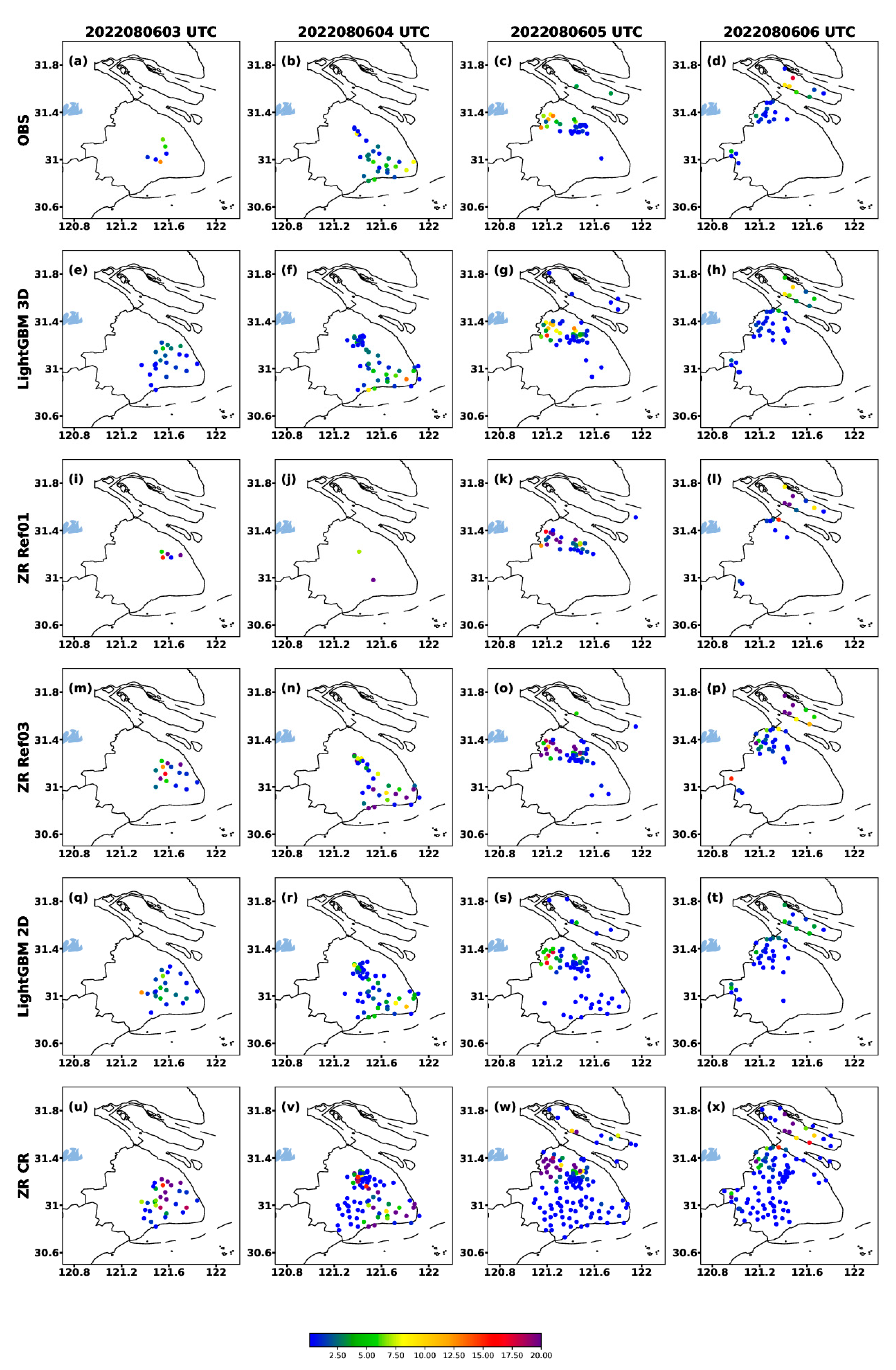
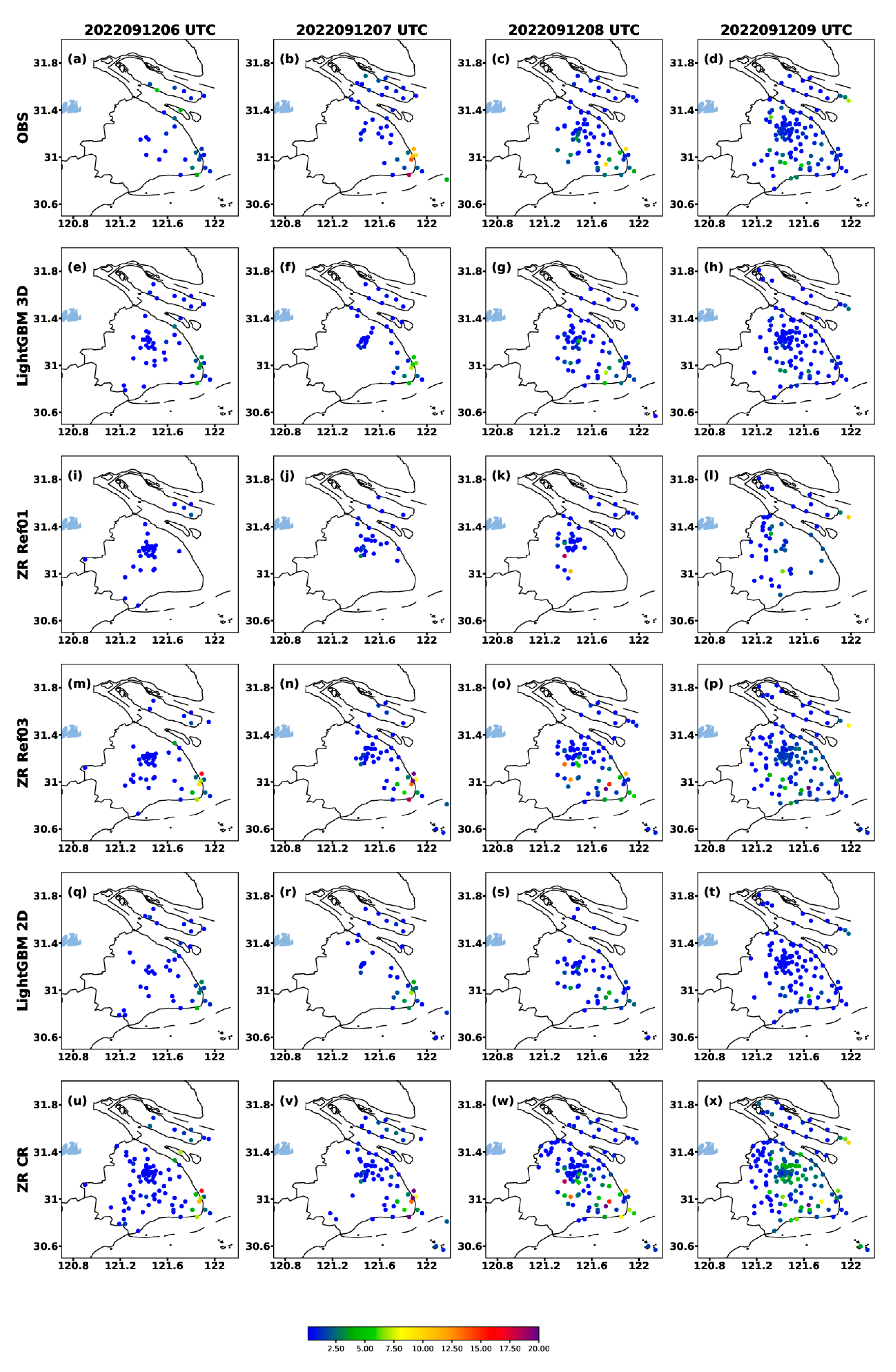
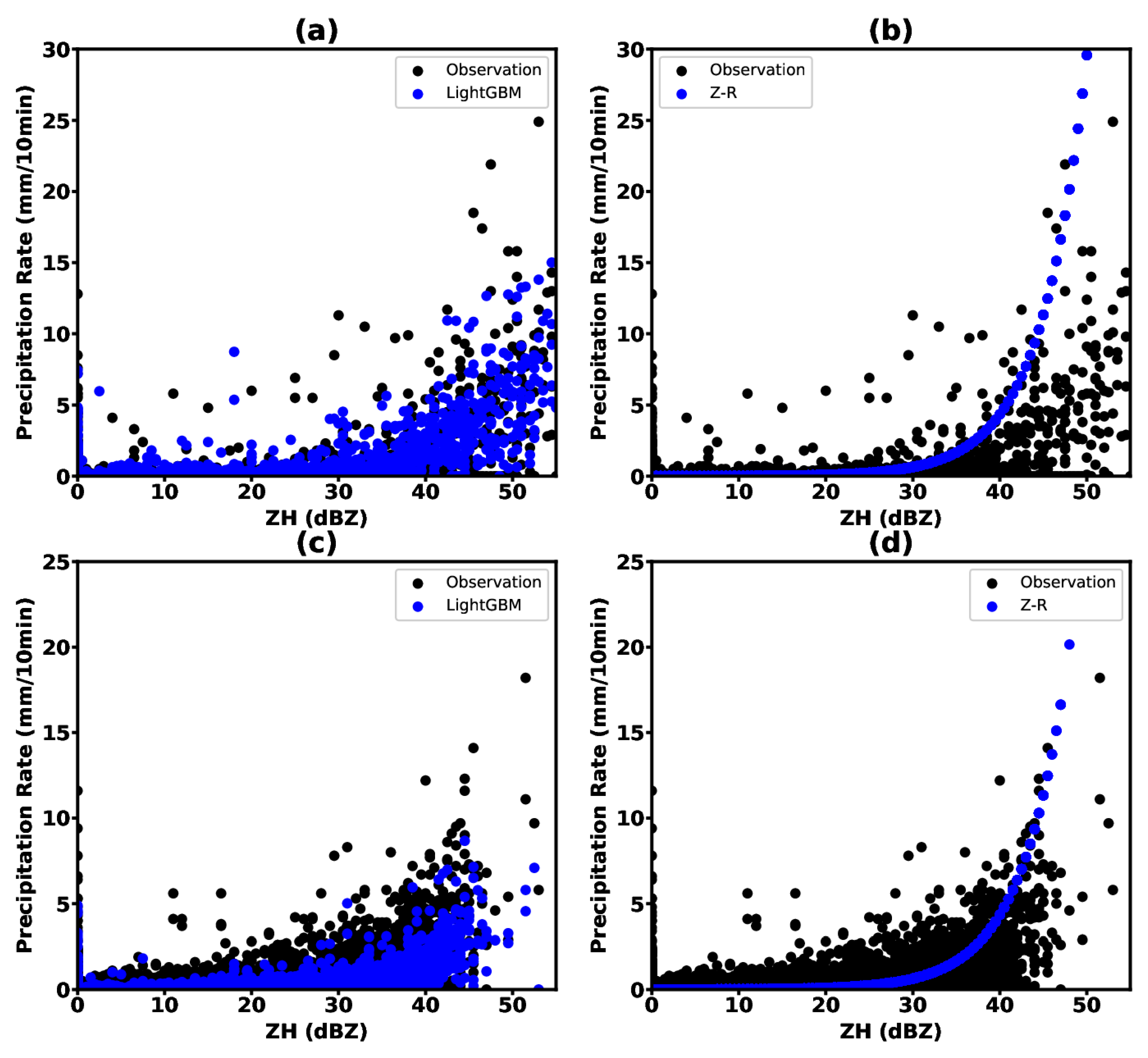
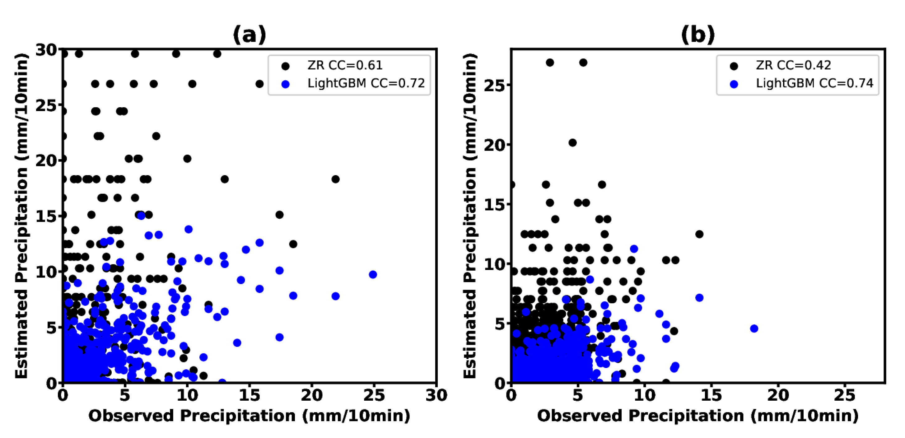
Affected by various weather systems, the precipitation that occurred in the Shanghai area from August to October 2022 showed different characteristics. The convective precipitation was predominant in August 2022, while the precipitation associated with typhoon systems occurred mainly from September to October 2022. In order to explore the ability of estimation models to perform on different types of precipitation, two sets of training-estimating datasets were established in this study. In the first dataset, we used the rainfall–radar data from June to July 2022 as the training data, while the rainfall–radar data from August 2022 were used as the testing data to explore the ability of the estimation models to estimate the convective rainfall. In the second dataset, we used the rainfall–radar data from June to August 2022 as the training data and the rainfall–radar data from September to October 2022 as the testing data to explore the ability of the estimation models to estimate the precipitation caused by typhoon systems.

Table 2 presents the skill scores of the MAE, MSLE, R² score, and CORR for the ten groups of experiments using the testing dataset in August 2022. As shown in Table 2, the LightGBM 3D model with the surrounding nine points (Exe 2) shows the best ability for the estimation of convective precipitation with the highest CORR (0.722) and lowest MAE (0.015) and MSLE (0.004). This can be attributed to the consideration of spatial offset during the model building process in Exe 2. Generally, the LightGBM 3D models outperform the LightGBM 2D model due to their higher CORR and R² scores closer to 1. In the Z–R relationship method, the MAE and MSLE increase with the height, while the CORR increases and reaches its maximum at 2000 m (Ref03) and then decreases with the height. In terms of convective precipitation, the LightGBM models demonstrate superior estimating performance compared to the Z–R relationship methods. The traditional Z–R relationship produced larger a MAE and MSLE, especially at 3000 m (Ref05), and a lower CORR, especially at 500 m (Ref00).

Table 3. As in Table 2 except for the testing dataset during September–October 2022.

Algorithm	Experiments	Description	MAE	MSLE	R2 Score	CORR
LightGBM 3D	Exe 1	24 levels 1 point	0.022	0.006	0.396	0.653
	Exe 2	24 levels 9 points	0.021	0.005	0.491	0.739
LightGBM 2D	Exe 3	CR 9 points	0.023	0.007	0.328	0.616
Z–R	Exe 4	Z–R Ref00	0.027	0.010	−0.121	0.337
	Exe 5	Z–R Ref01	0.029	0.007	−0.658	0.547
	Exe 6	Z–R Ref02	0.031	0.006	−4.565	0.424
	Exe 7	Z–R Ref03	0.028	0.006	−1.048	0.619
	Exe 8	Z–R Ref04	0.028	0.006	−0.537	0.604
	Exe 9	Z–R Ref05	0.028	0.007	−0.345	0.583
	Exe 10	Z–R CR	0.064	0.015	−31.059	0.255

displays the skill scores of the MAE, MSLE, R² score, and CORR of the ten groups of the experiments for the testing dataset from September to October 2022. Similar to the previous findings, the LightGBM models outperform the Z–R relationship methods in terms of estimating performance. As shown in Table 3, the LightGBM 3D model with the surrounding nine points (Exe 2) achieves the highest CORR (0.739) and the lowest MAE (0.021) and MSLE (0.005) for the testing dataset from September to October 2022. Notably, compared to the convective precipitation, all three LightGBM models produced larger estimation errors for the testing dataset from September to October 2022 in which the precipitation was mainly caused by typhoon systems. This means that the LightGBM 3D models demonstrate a more accurate estimation of convective precipitation compared to precipitation caused by typhoon systems. This finding suggests that the model performs better in capturing the characteristics and patterns associated with convective rainfall.

Figure 4 describes the scatter distributions of the 10 min cumulative precipitation estimated with the LightGBM 3D model and Z–R relationship method against the reflectivity of the radar data. Figure 4a,b illustrates the scatterplots for the testing dataset in August, and Figure 4c,d shows the scatterplots for the testing dataset from September to October. As shown in Figure 4a, the LightGBM 3D model produces more realistic QPEs for convective precipitation than the traditional Z–R method. However, for the precipitation with a 10 min cumulative precipitation greater than 15 mm, the LightGBM 3D model estimates a smaller precipitation than the observed rainfall. For the precipitation in September, which is mainly caused by typhoon systems, the estimating ability of the LightGBM 3D model has decreased (Figure 4c) and manifested as an underestimation of the precipitation. The Z–R relationship method has a serious overestimation for the precipitation, with a 10 min cumulative precipitation greater than 10 mm (Figure 4b,d), resulting in a large MAE and MSLE.

Figure 5 describes the scatterplots of the LightGBM 3D QPEs and Z–R QPEs versus the observed 10 min cumulative precipitation. The LightGBM 3D model produced a higher CORR than the traditional Z–R relationship method for both the convective precipitation and typhoon system-induced precipitation. However, the LightGBM 3D model underestimates the precipitation caused by typhoon systems as well as the convective precipitation, with the accumulated precipitation exceeding 15 mm in 10 min.

Figure 6 illustrates the frequency distribution of the precipitation bias between the rain gauge observation and the estimation from the four methods. For the LightGBM 3D model, most of the bias values are less than 0 mm/10 min, with the maximum frequency (about 67%) at the difference between −2.5 and 0 mm/10 min. The frequency of the bias values between −2.5 and 2.5 mm/10 min is about 91%, which is the highest among the results of the four methods. In addition, the CORR of the LightGBM 3D model results is about 0.72, which is also the largest among the four methods (Figure 6a). These statistics further demonstrate that the estimation accuracy of the LightGBM 3D model is the highest among the four methods. Regarding the LightGBM 2D estimates, the frequency distribution of the bias values is similar to that of the LightGBM 3D model except that the frequency (about 90%) decreases slightly at the differences between −2.5 and 2.5 mm/10 min and increases somewhat at the differences between −10 and −2.5 mm/10 min. Additionally, the CORR of the LightGBM 2D estimates is about 0.60, which is also lower than that of the LightGBM 3D (Figure 6c).

As for the Z–R Ref02 estimates, the maximum frequency (about 61%) is still at the difference between −2.5 and 0 mm/10 min, and the frequency of the bias values between −2.5 and 2.5 mm/10 min is about 84%, which is less than the LightGBM 3D and the LightGBM 2D model (Figure 6b). In terms of the Z–R CR estimates, most of the bias values shift to more than 0 mm/10 min, the frequency of the differences between −2.5 and 2.5 mm/10 min decreases to about 77%, and that of the differences exceeding 20 mm/10 min increases remarkably. Moreover, the CORR of the Z–R CR estimates is only 0.54.

The above statistics suggest that the LightGBM method obviously improves the QPE accuracy compared to the Z–R relationship method. After introducing the LightGBM 3D model, the biases between the observations and estimations decrease, and the correlation between the observations and estimations increases remarkably. Therefore, the LightGBM 3D model proposed in this research performs the best for precipitation estimation compared to the other methods discussed above.

Figure 7 shows the MAE and MSLE of the radar QPE from the different methods for different thresholds of precipitation in August 2022. The MAE values for the different methods increase gradually with the increase in the precipitation rate (Figure 7a), implying that the biases of the QPE from the observations increase with increasing precipitation intensity. The LightGBM methods perform better than the Z–R relationship methods for the estimations of the overall precipitation due to their lower MAE and MSLE values for all the rainfall intensities. Among the whole methods, the LightGBM 3D model produces the lowest MAE and MSLE values for all the rainfall intensities, indicating the best performance for the whole thresholds of precipitation. Compared to the other rainfall intensities, the LightGBM 3D model has the largest MAE and MSLE values for a rainfall rate larger than 10 mm/10 min, indicating its worst performance for extreme precipitation.

4.2.2. Case Study

To access the performance of various radar QPE methods proposed in this study on the spatial distribution, two types of heavy rainfall cases were selected this study: One occurred on 6 August 2022 that is representative of the convective precipitation, and the other occurred on 12 September 2022 that is representative of the typhoon-systems-induced rainfall. The composite reflectivity (CR) values of the two cases are illustrated in Figure 8. For the case that occurred at 0300 UTC 6 August 2022, the radar echoes mainly appeared at Pudong and Nanhui, Shanghai (Figure 8a), with the maximum reflectivity exceeding 60 dBZ. Subsequently, the echoes continued to develop and triggered new convection in the surrounding area. At 0500 and 0600 UTC, the echoes appeared to the north of Shanghai, resulting in heavy rainfall in these areas. Notably, there is a large range of non-precipitation echoes in the south of Shanghai. Regarding the case on 12 September 2022, a heavy rainstorm occurred in Shanghai due to the external inverted trough and the main body of the severe Typhoon Muifa. The radar echoes mainly appeared in the northeast of Shanghai, with the maximum reflectivity exceeding 50 dBZ (Figure 8f) and the precipitation intensity exceeding 18 mm/10 min.

Figure 9 shows the observed rainfall and the radar QPEs obtained from five methods at 0300, 0400, 0500, and 0600 UTC 6 August 2022. The results from the above methods can reproduce at least some aspects in the convective rainfall case. The LightGBM 3D model can reproduce a more realistic range of observed rainfall. However, whether the Z–R relationship methods can reproduce the rainfall range depends on which layer of reflectivity it uses for the radar QPE. For example, the Z–R Ref03 method produces a more reasonable rainfall range compared to the Z–R Ref01 method. The LightGBM 3D model also produces a more realistic intensity of the convective rainfall case with lower biases. However, both Z–R Ref01 (Figure 9j,k) and Z–R Ref03 (Figure 9n,o) remarkably overestimate the precipitation intensity of this convective rainfall case. Although both of the following QPE methods are based on composite reflectivity (CR), the LightGBM 2D model can reproduce a more reasonable range and intensity of precipitation compared to the Z–R CR method. The Z–R CR method has estimated a large range of false precipitation in the non-precipitation echo areas that appeared to the south of Shanghai (Figure 9v,w), which also indicates that the precise quality control of radar data is required when using the Z–R CR method for precipitation estimation. Different from the Z–R CR method, the LightGBM 2D model barely estimates false precipitation in the non-precipitation echo areas, possibly due to its automatic quality control on radar data during the model training. Moreover, compared to the LightGBM 2D model, the LightGBM 3D model based on the multi-level radar data can estimate a more refined spatial structure and accurate intensity of rainfall. Overall, the radar QPE results from the LightGBM 3D model are the most realistic compared to the observations for both the rainfall intensity and spatial distribution.

Figure 10 analyzes the observed rainfall and the radar QPE obtained from five methods at 0600, 0700, 0800, and 0900 UTC 12 September 2022 during Typhoon Muifa. Similar to the above case, the Z–R method obviously overestimates the rainfall intensity (Figure 10o) and significantly estimates a larger rainfall range (Figure 10u). The LightGBM 3D model accurately estimates the location of the center of heavy precipitation in the eastern coastal area of Shanghai at 0700 UTC but underestimates the precipitation intensity. This might be because of the lack of rainfall samples caused by the typhoon systems in the training dataset where there are multiple convective precipitation samples. In the rainfall events caused by typhoon systems, relatively small reflectivity values can generate heavy precipitation, while in the convective precipitation events, the reflectivity values that generate heavy precipitation are often larger. For example, for the convective rainfall case that occurred at 0600 UTC 6 August 2022, the maximum precipitation rate reached 17.4 mm/10 min with the maximum reflectivity >65 dBZ. However, for the rainfall case caused by the typhoon system at 0700 UTC 12 September 2022, the maximum precipitation rate reached 18.2 mm/10 min with the maximum reflectivity only exceeding 50 dBZ.

5. Conclusions and Discussion

In this study, we propose a method for quantitative precipitation estimation (QPE) using the new generation 3D grid and mosaic weather radar network data. The method is based on the LightGBM machine learning algorithm, which is a computationally efficient gradient boosting decision tree algorithm. The radar reflectivity data from 24 vertical levels were selected to feed the LightGBM 3D model. Moreover, to mitigate the impact of spatial offset on the QPE model, we selected the reflectivity data from nine points surrounding the rain gauge station. In addition, the location and time information from the rain gauge station were input into the model as the category features. As a result, the diurnal variation and geographic attribute characteristics of the rain gauge station were taken into account during the estimating process. Furthermore, the LightGBM model is explainable by using the SHAP regression values to evaluate the contribution of the input features. In order to further evaluate the performance of the LightGBM 3D model with nine points (Exe 2), it was compared with the other nine methods: the LightGBM 3D model with a single point (Exe 1), the LightGBM 2D model based on the composite reflectivity (Exe 3), and various Z–R relationship methods obtained from Ref00 to Ref05 (Exe 4 to Exe 9), as well as the Z–R relationship based on composite reflectivity (Exe 10). Moreover, to further assess the performance of various radar QPE methods on the spatial distribution, two types of heavy rainfall cases, including the convective rainfall event and the rainfall event caused by typhoon systems, were selected in this study. Both the statistical analysis and the spatial distribution results demonstrate that the LightGBM 3D model with nine points performs the best in terms of quantitative precipitation estimation in this study. The main conclusions are as follows:

(1)

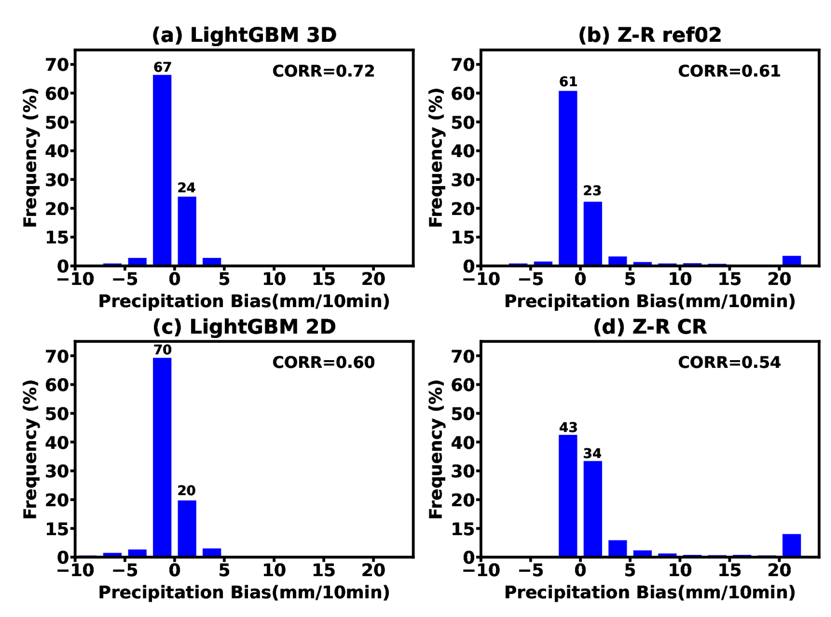
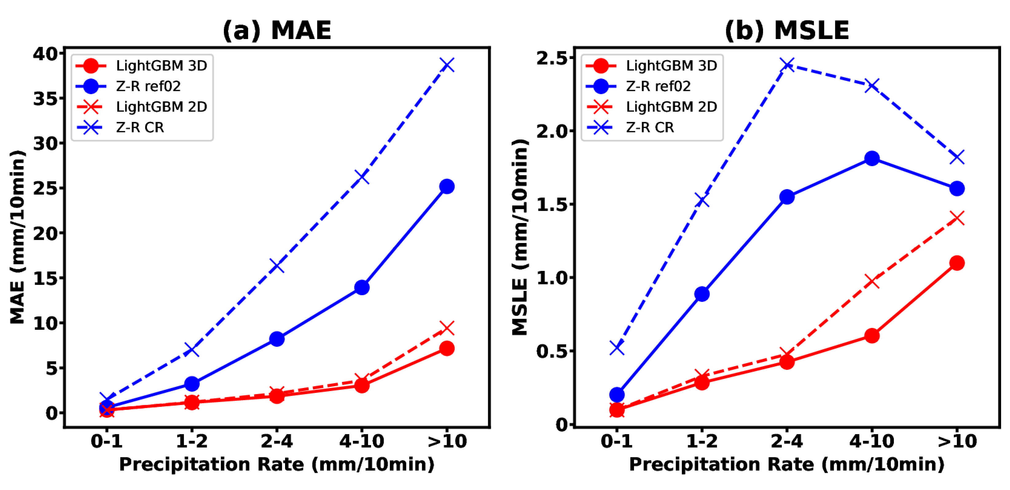
The statistical analysis results indicate that the LightGBM 3D model with nine points shows the best ability for the QPE due to its highest correlation (CORR) and R-squared (R²) scores, as well as the lowest mean absolute error (MAE) and mean squared logarithmic error (MSLE). Conversely, the Z–R relationship method based on composite reflectivity (CR) shows the worst performance for the radar QPE in this study.

(2)

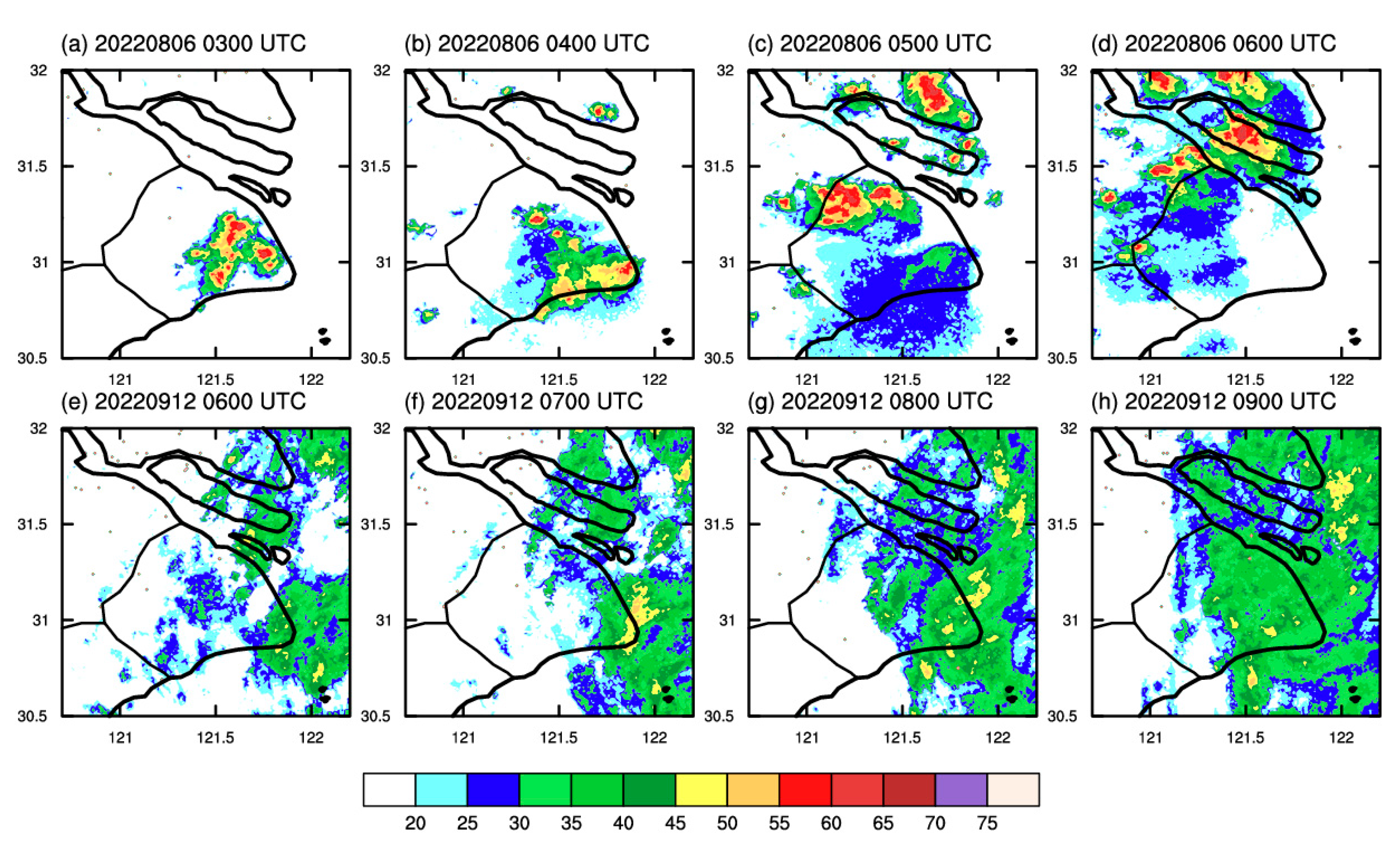
The spatial distribution results from the two type cases demonstrate that the LightGBM 3D model with nine points can reproduce a more realistic range and intensity of the observed rainfall, while the Z–R relationship method (especially the Z–R CR method) tends to significantly overestimate the range and intensity of heavy rainfall. However, the LightGBM models tend to underestimate extreme rainfall, which is perhaps due to the “long tail effect” caused by the limited number of extreme precipitation samples.

(3)

In this study, the Z–R CR method estimated a large range of false precipitation in the non-precipitation echo areas, resulting in its overestimation of the range of rainfall. Different from the Z–R CR method, neither the LightGBM 3D model nor the LightGBM 2D model can estimate a realistic precipitation range or minimally estimate the false precipitation in the non-precipitation echo areas. This suggests that the LightGBM methods may have an automatic quality control effect on the non-precipitation echoes of radar data, enhancing the model stability and reducing the impact of the radar data quality.

(4)

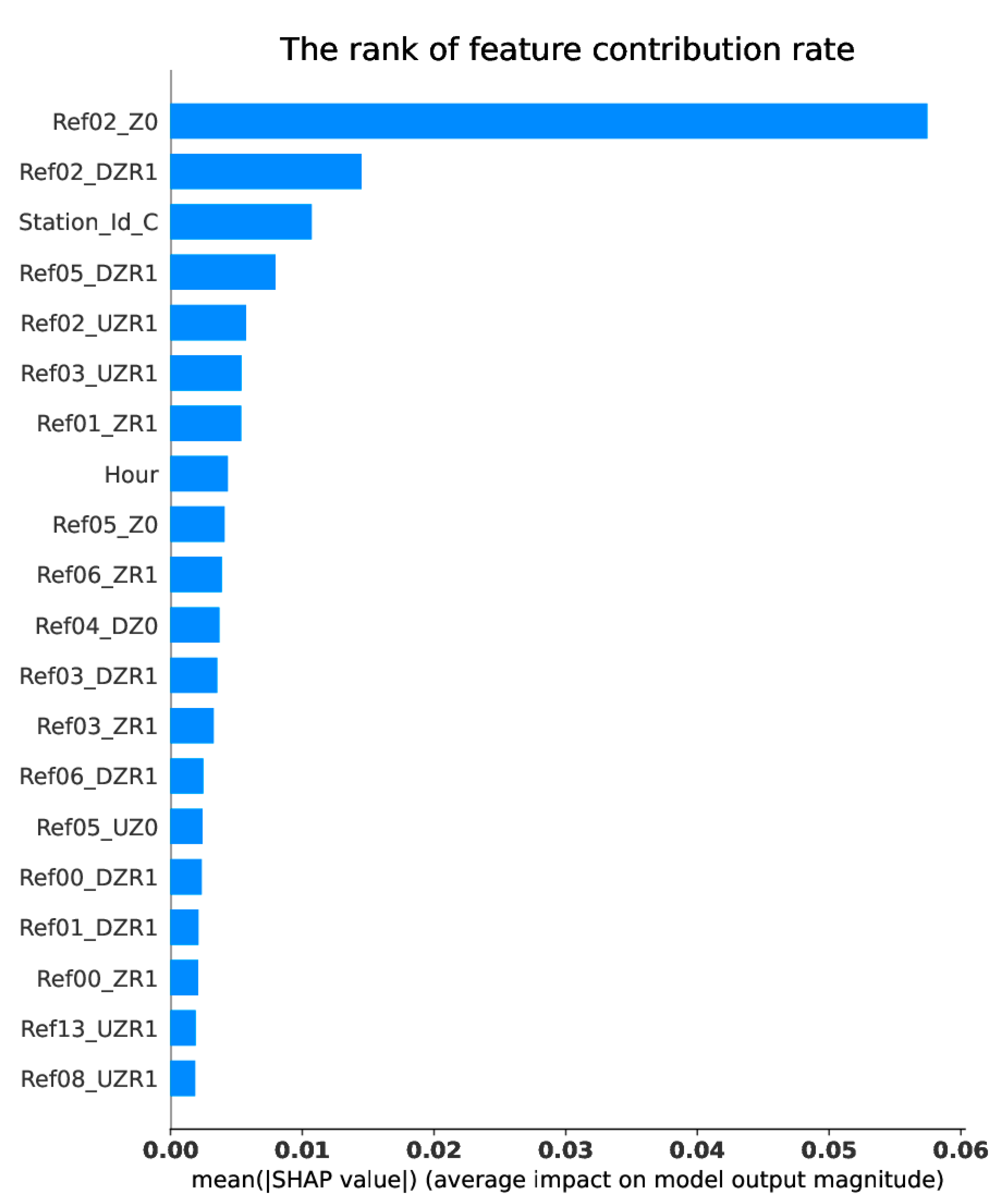
The advantages of the LightGBM 3D model can be attributed not only to the inclusion of multi-level reflectivity in its training but also to its consideration of the geographic attributes of the rain gauge stations, diurnal variation characteristics, and the influence of mitigating spatial offset. The SHAP magnitude further highlights that the geographic attributes of the rain gauge stations (Station_Id_C) and the diurnal variation (Hour) characteristics make significant contributions to the LightGBM 3D model (Figure 2 and Figure 3).

(5)

The LightGBM 3D model exhibits an accurate estimation of convective precipitation; however, it tends to underestimate the intensity of precipitation caused by typhoon systems. This discrepancy may be attributed to the differing radar reflectivity characteristics between convective precipitation and typhoon-induced precipitation. Convective rainfall events typically exhibit high reflectivity values, whereas, in typhoon systems, heavy precipitation can occur without significantly strong reflectivity. Additionally, the training process includes multiple convective precipitation samples but lacks sufficient rainfall samples caused by typhoon systems, leading to a slight underestimation in typhoon-induced precipitation.

References

1. Zou, H.B.; Wu, S.S.; Tian, M.X. Radar quantitative precipitation estimation based on the Gated Recurrent Unit neural network and echo-top data. Adv. Atmos. Sci. 2023, 38, 1750–1762. [Google Scholar] [CrossRef]
2. Martinaitis, S.M.; Osborne, A.P.; Simpson, M.J.; Zhang, J.; Howard, K.W.; Cocks, S.B.; Kaney, B.T. A physically based multisensor quantitative precipitation estimation approach for gap-filling radar coverage. J. Hydrometeorol. 2020, 21, 1485–1511. [Google Scholar] [CrossRef]
3. Zhang, J.; Tang, L.; Cocks, S.; Zhang, P.; Ryzhkov, A.; Howard, K.; Langston, C.; Kaney, B. A dual-polarization radar synthetic QPE for operations. J. Hydrometeorol. 2020, 21, 2507–2521. [Google Scholar] [CrossRef]
4. Zhang, Y.; Liu, L.; Wen, H. Performance of a radar mosaic quantitative precipitation estimation algorithm based on a new data quality index for the Chinese Polarimetric Radars. Remote Sens. 2020, 12, 3557. [Google Scholar] [CrossRef]
5. Jin, B.; Wu, Y.; Miao, B.; Wang, X.L.; Guo, P. Bayesian spatiotemporal modeling for blending in situ observations with satellite precipitation estimates. J. Geophys. Res. Atmos. 2014, 119, 1806–1819. [Google Scholar] [CrossRef]
6. Zhang, G.; Tian, G.; Cai, D.; Bai, R.; Tong, J. Merging radar and rain gauge data by using spatial–temporal local weighted linear regression kriging for quantitative precipitation estimation. J. Hydrol. 2021, 601, 126612. [Google Scholar] [CrossRef]
7. Shao, Y.; Fu, A.; Zhao, J.; Xu, J.; Wu, J. Improving quantitative precipitation estimates by radar-rain gauge merging and an integration algorithm in the Yishu River catchment, China. Theor. Appl. Climatol. 2021, 144, 611–623. [Google Scholar] [CrossRef]
8. Marshall, J.S.; Palmer, W. The distribution of raindrops with size. J Meteor. 1948, 5, 165–166. [Google Scholar] [CrossRef]
9. Fujiwara, M. Raindrop-size distribution from individual storms. J. Atmos. Sci. 1965, 22, 585–591. [Google Scholar] [CrossRef]
10. Martens, B.; Cabus, P.; Jongh, I.D.; Verhoest, N. Merging weather radar observations with ground-based measurements of rainfall using an adaptive multiquadric surface fitting algorithm. J. Hydrol. 2013, 500, 84–96. [Google Scholar] [CrossRef]
11. Jorgensen, D.P.; Willis, P.T. A Z-R relationship for hurricanes. J. Appl. Meteorol. Climatol. 1982, 21, 356–366. [Google Scholar] [CrossRef]
12. Lee, G.W. Sources of errors in rainfall measurements by Polarimetric radar: Variability of drop size distributions, observational noise, and variation of relationships between R and Polarimetric parameters. J. Atmos. Ocean. Technol. 2006, 23, 1005–1028. [Google Scholar] [CrossRef]
13. Wu, W.X.; Zou, H.B.; Shan, J.S.; Wu, S.S. A dynamical Z-R relationship for precipitation estimation based on radar echo-top height classification. Adv. Meteorol. 2018, 2018, 8202031. [Google Scholar] [CrossRef]
14. Huang, H.; Zhao, K.; Chen, H.; Hu, D.; Fu, P.; Lin, Q.; Yang, Z. Improved attenuation-based radar precipitation estimation considering the azimuthal variabilities of microphysical properties. J. Hydrometeorol. 2020, 21, 1605–1620. [Google Scholar] [CrossRef]
15. Kim, T.J.; Kwon, H.H.; Kim, K.B. Calibration of the reflectivity-rainfall rate (ZR) relationship using long-term radar reflectivity factor over the entire South Korea region in a Bayesian perspective. J. Hydrol. 2021, 593, 125790. [Google Scholar] [CrossRef]
16. Wang, G.; Liu, L.; Ding, Y. Improvement of Radar Quantitative Precipitation Estimation Based on Real-Time Adjustments to Z--R Relationships and Inverse Distance Weighting Correction Schemes. Adv. Atmos. Sci. 2012, 29, 575–584. [Google Scholar] [CrossRef]
17. Alfieri, L.; Claps, P.; Laio, F. Time-dependent Z-R relationships for estimating rainfall fields from radar measurements. Nat. Hazards Earth Syst. Sci. 2010, 10, 149–158. [Google Scholar] [CrossRef]
18. Kuang, Q.M.; Yang, X.B.; Zhang, W.S.; Zhang, G.P. Spatiotemporal modeling and implementation for radar-based rainfall estimation. IEEE Geosci. Remote Sens. Lett. 2016, 13, 1601–1605. [Google Scholar] [CrossRef]
19. Wolfensberger, D.; Gabella, M.; Boscacci, M.; Germann, U.; Berne, A. RainForest: A random forest algorithm for quantitative precipitation estimation over Switzerland. Atmos. Meas. Tech. 2021, 14, 3169–3193. [Google Scholar] [CrossRef]
20. Suykens, K.J.A.; Vandewalle, J. Least squares support vector machine classifiers. Neural Process. Lett. 1999, 9, 293–300. [Google Scholar] [CrossRef]
21. Sehad, M.; Lazri, M.; Ameur, S. Novel SVM-based technique to improve rainfall estimation over the Mediterranean region (north of Algeria) using the multispectral MSG SEVIRI imagery. Adv. Space Res. 2017, 59, 1381–1394. [Google Scholar] [CrossRef]
22. Hilburn, K.A.; Ebert-Uphoff, I.; Miller, S.D. Development and interpretation of a neural-network-based synthetic radar reflectivity estimator using GOES-R satellite observations. J. Appl. Meteorol. Clim. 2021, 60, 3–21. [Google Scholar] [CrossRef]
23. Mayer, K.J.; Barnes, E.A. Subseasonal forecasts of opportunity identified by an explainable neural network. Geophys. Res. Lett. 2021, 48, e2020GL092092. [Google Scholar] [CrossRef]
24. McGovern, A.; Lagerquist, R.; John Gagne, D.; Jergensen, G.E.; Elmore, K.L.; Homeyer, C.R.; Smith, T. Making the black box more transparent: Understanding the physical implications of machine learning. Bull. Am. Meteorol. Soc. 2019, 100, 2175–2199. [Google Scholar] [CrossRef]
25. Silva, S.J.; Keller, C.A.; Hardin, J. Using an explainable machine learning approach to characterize Earth System model errors: Application of SHAP analysis to modeling lightning flash occurrence. J. Adv. Model. Earth Syst. 2022, 14, e2021MS002881. [Google Scholar] [CrossRef]
26. Toms, B.A.; Barnes, E.A.; Hurrell, J.W. Assessing decadal predictability in an Earth-System model using explainable neural networks. Geophys. Res. Lett. 2021, 48, e2021GL093842. [Google Scholar] [CrossRef]
27. Chen, T.; Guestrin, C. XGBoost: A Scalable Tree Boosting System. In Proceedings of the 22nd ACM SIGKDD International Conference on Knowledge Discovery and Data Mining, San Francisco, CA, USA, 13–17 August 2016; ACM: New York, NY, USA, 2016; pp. 785–794. [Google Scholar]
28. Stirnberg, R.; Cermak, J.; Kotthaus, S.; Haeffelin, M.; Andersen, H.; Fuchs, J. Meteorology-driven variability of air pollution (PM1) revealed with explainable machine learning. Atmos. Chem. Phys. 2021, 21, 3919–3948. [Google Scholar] [CrossRef]
29. Grinsztajn, L.; Oyallon, E.; Varoquaux, G. Why do tree-based models still outperform deep learning on typical tabular data? Adv. Neural Inf. Process. Syst. 2022, 35, 507–520. [Google Scholar]
30. Li, S.; Qin, J.; He, M.; Paoli, R. Fast Evaluation of Aircraft Icing Severity Using Machine Learning Based on XGBoost. Aerospace 2020, 7, 36. [Google Scholar] [CrossRef]
31. Ke, G.; Meng, Q.; Finley, T.; Wang, T.; Chen, W.; Ma, W.; Ye, Q.W.; Liu, T.Y. LightGBM: A highly efficient gradient boosting decision tree. Adv. Neural Inf. Process. Syst. 2017, 30, 3146–3154. [Google Scholar]
32. Han, L.; Sun, J.; Zhang, W.; Xiu, Y.; Feng, H.; Lin, Y. A machine learning nowcasting method based on real-time reanalysis data. J. Geophys. Res. Atmos. 2017, 122, 4038–4051. [Google Scholar] [CrossRef]
33. Yu, Y.; Gille, S.T.; Sandwell, D.T. Global mesoscale ocean variability from multiyear altimetry: An analysis of the influencing factors. Artif. Intell. Earth Syst. 2022, 1, e210008. [Google Scholar] [CrossRef]
34. Qian, Q.F.; Jia, X.J.; Lin, H. Seasonal forecast of non-monsoonal winter precipitation over the Eurasian continent using machine-learning models. J. Clim. 2021, 34, 7113–7129. [Google Scholar] [CrossRef]
35. Devore, J.L. Probability and Statistics for Engineering and the Sciences; Cengage Learning: Boston, MA, USA, 2011; p. 768. [Google Scholar]
36. Lundberg, S.M.; Erion, G.; Chen, H.; DeGrave, A.; Prutkin, J.M.; Nair, B. From local explanations to global understanding with explainable AI for trees. Nat. Mach. Intell. 2020, 2, 56–67. [Google Scholar] [CrossRef]
37. Molnar, C. Interpretable Machine Learning: A Guide for Making Black Box Models Explainable; Leanpub: Victoria, BC, Canada, 2019. [Google Scholar]
Figure 1. The location of (a) rain gauges (depicted as blue dots) within the study area, (b) LightGBM method with surrounding 9 points, and (c) LightGBM method with single point.
Atmosphere 14 01364 g001
Figure 2. The Shapley additive explanations (SHAP) magnitude for the LightGBM 3D model with single points (Exe 1).
Atmosphere 14 01364 g002
Figure 3. The top 20 input variables with the largest SHAP value magnitudes by Shapley additive explanations (SHAP) magnitude for the LightGBM 3D model with 9 points (Exe 2).
Atmosphere 14 01364 g003
Figure 4. Scatterplots of 10 min cumulative precipitation with LightGBM 3D (a,c) and Z–R (b,d) against the reflectivity of radar data for the testing dataset in August 2022 (a,b) and the testing dataset during September–October 2022 (c,d).
Atmosphere 14 01364 g004
Figure 5. Scatterplots of LightGBM 3D QPEs and Z–R QPEs versus the observed 10 min cumulative precipitation for the testing dataset in August 2022 (a) and the testing dataset during September–October 2022 (b).
Atmosphere 14 01364 g005
Figure 6. The frequency of precipitation difference between the rain gauge observation and QPE obtained from LightGBM 3D (a), Z–R ref02 (b), LightGBM 2D (c), and Z–R CR in August 2022 (d).
Atmosphere 14 01364 g006
Figure 7. The (a) MAE and (b) MSLE of radar QPE obtained from different methods for different thresholds of precipitation in August 2022.
Atmosphere 14 01364 g007
Figure 8. The composite reflectivity (CR) values (dBZ) obtained from weather radar network data at 0300 UTC (a), 0400 UTC (b), 0500 UTC (c), 0600 UTC (d) 6 August 2022 and 0600 UTC (e), 0700 UTC (f), 0800 UTC (g), 0900 UTC (h) 12 September 2022.
Atmosphere 14 01364 g008
Figure 9. The observed rainfall (ad) and the radar QPE (mm/10 min) obtained from LightGBM 3D (eh), Z–R Ref01 (il), Z–R Ref03 (mp), LightGBM 2D (qt), and Z–R CR (ux) at 0300, 0400, 0500 and 0600 UTC 6 August 2022.
Atmosphere 14 01364 g009
Figure 10. As in Figure 9 except for 0600, 0700, 0800, and 0900 UTC 12 September 2022.
Atmosphere 14 01364 g010