Abstract
This paper presents the extent to which the combination of extra-atmospheric and hydroclimatic factors can be deciphered to record their contribution to the evolution and forecasting of the Danube discharge (Q) in the lower basin. A combination of methods such as wavelet filtering and deep learning (DL) constitutes the basic method for discriminating the external factors (solar activity through Wolf numbers) that significantly contribute to the evolution and prediction of the lower Danube discharge. An ensemble of some of the most important factors, namely, those representing the atmospheric components, i.e., the Greenland-Balkan Oscillation Index (GBOI) and the North Atlantic Oscillation Index (NAOI); the hydroclimatic indicator, the Palmer Hydrological Drought Index (PHDI); and the extra-atmospheric factor, constitutes the set of predictors by means of which the predictand, Q, in the summer season, is estimated. The external factor has to be discriminated in the Schwabe and Hale spectra to make its convolutional contribution to the Q estimation in the lower Danube basin. An interesting finding is that adding two solar predictors (associated with the Schwabe and Hale cycles) to the terrestrial ones give a better estimation of the Danube discharge in summer, compared to using only terrestrial predictors. Based on the Nash–Sutcliffe (NS) index, a measure of performance given by the extreme learning machine (ELM), it is shown that, in association with certain terrestrial predictors, the contribution of the Hale cycle is more significant than the contribution of the Schwabe cycle to the estimation of the Danube discharge in the lower basin.
1. Introduction
In recent investigations, in particular, a considerable number of papers have been devoted to the study of complex natural geophysical systems. In nature, there are diverse systems that interact (directly or indirectly, for example the Solar System with its component, the geophysical system) with each other and are modeled as systems of networks of coupled oscillators [1]. Time series describing the evolution of natural phenomena have entered the sphere of neuroscience processing. The physical mechanisms arising from multiple interactions are generally unknown and/or well hidden (Tirabassi et al., 2015) [1] or involve prohibitive calculations. Deterministic models, however, are still limited. As stated in [2,3], the direction of causality of climate change is not clear.
The method of investigation of these natural phenomena is one of the reasons for the controversy. For example, while Tirabassi et al. [1] focused on the similarity of evolution over different periods of time, Tupikina et al. [4] were concerned with the change points that characterize climate evolution.
It is generally known that the influence of solar activity on terrestrial variables is nonlinear and nonstationary. Mares et al. [5] found that the link between the Wolf number and the main climate indices is nonlinear. This conclusion was reached by comparing the linear Pearson correlation coefficient |R| with the nonlinear correlation coefficient (NLR). The NLR coefficient is calculated according to mutual information (MI), which is based on information entropy [6,7]. Several studies have detailed the performance of nonlinear correlation in comparison with classical linear correlation [8,9].
Attempts to simplify either deterministic or stochastic computational models have not led to encouraging results. The advent of high-performance computers has changed the balance of investigations in favor of nonlinear methods describing the evolution of hydroclimatic phenomena in their natural interaction. Not surprisingly, the first experiment developed on a computer was preceded by the publication of L. F. Richardson’s “Weather Prediction by Numerical Process” in 1922, whose idea formed the basis of the integration of the air dynamics equations [10], almost 30 years later by Charney et al. [11]. Richardson’s dream through the efforts of his meteorological followers became a quantitative science that is today “partly recognized” by the Nobel Prize awarded to Syukuro Manabe and Klaus Hasselmann in 2021.
Of course, hydrological prediction depends to a large extent on weather phenomena and their evolution. The climate system under the impact of solar activity has an evolution that is very difficult to predict using deterministic models due to the chaotic state of the solar dynamo and the high nonlinearity of physical processes on the Sun [3]. Therefore, statistical methods are mainly used to investigate the solar impact on geophysical processes.
In particular, hydrological variables are even more difficult to take into account in global climate models [2]. And, the results of investigations so far have been quite controversial for this reason. In general, there are pros and cons for the different statistical methods, but the most appropriate ones should be used/combined.
This is because the Sun acts on the geophysical system through a cascade of scales, and in a complex way, so that the impact on climate/hydrological components is realized indirectly through other geophysical components [12,13,14,15].
There have been multiple attempts to discriminate the solar external factor under the aspect of its involvement in global climate models [16,17] or under the aspect of direct stochastic modeling.
In terms of unifying classical time series correlative methods of investigation, there have been some robust attempts in the geophysical field with so-called “smart regressions” [18] for linear links. But, the solar impact on the geophysical environment has a pronounced nonlinear character [15,19,20]. This latter shortcoming has been successfully resolved for investigations of nonlinear linkages [21,22,23,24].
The present study starts from the fact that, until now, the following have not been addressed:
- -
- The minimum number of factors that form a sufficiently predictive ensemble and that belong to different systems (atmosphere, hydrosphere, external (Solar system)) has not been detected.
- -
- It has not been possible to clearly discriminate between the impact of the different spectral components (solar cycles of 11 and 22 years respectively) on the geophysical system.
- -
- No neural network has been used for the prognostic differentiation of solar cycle components with their characteristic impact on the hydrological evolution of major European rivers.
The main aim of this investigation is to see and highlight the differentiated impact of different cyclic components of the solar spectral activity.
The specific hypothesis is that the differentiated solar impact as a predictor also produces differences in the predicted discharge (Q) in the Danube River, both in amplitude and phase.
In the present study, the solar activity is considered to act simultaneously via the two cycles (Schwabe or Hale) on the discharge, Q, in association with only one or more components of the climate system. The components of the climate system considered are the Greenland-Balkan Oscillation Index (GBOI), the North Atlantic Oscillation Index (NAOI) and the Palmer Hydrological Drought Index (PHDI).
Considering the holistic action of each of the solar cycles with the three predictors on the Danube discharge, we obtain an interesting result that is not easy to explain.
2. Material and Methods
Knowing that the variability of the Danube discharge is driven by internal factors of global/regional action, in the present study, besides the well-known climate index associated with the North Atlantic Oscillation, the main driver of hydrometeorological phenomena in western and northwestern Europe, the Greenland-Balkan Oscillation Index, whose influence is relevant in the Lower Danube Basin, as shown in the following, was considered. At the regional scale, the Palmer-type index was considered, which represents the state of moisture along the entire Danube basin. At the local scale and representing the dependent variable, the Danube River’s discharge was taken, as measured at Orsova, a station located at the entrance in Romania of the Danube River. For the natural external driver of the Danube discharge, the solar activity, quantified by the solar sunspot number (SSN), was taken. In the text of this paper, the terminology “Wolf number” is also used.
The applied methods are based on filters by means of the wavelet transform, as well as elements from the artificial intelligence domain, such as extreme deep learning (ELM).
2.1. Data
Five predictors and one predictand for seasonal time series during 1901-2000 were considered for the data. Two atmospheric predictors at the large scale, NAOI and GBOI, were considered, along with a hydroclimatic specific predictor of the Palmer type for drought and two predictors for solar activity. The NAOI data were taken from the Climate Research Unit (https://crudata.uea.ac.uk/cru/data/nao/values.html, accessed on 9 February 2023), and the GBOI data were calculated according to Mares et al. (2013) [25]. The PHDI was defined as PC1 of EOF decomposition from the 15 stations in the Danube Basin, presented in Figure 1, where the PHDI time series were developed. Details about the PHDI can be found in Mares et al., 2022 [26].
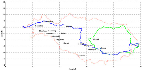
Figure 1.
The Danube basin with 15 stations considered for PHDI estimation. The location of Orsova station is marked with *.
The two extra-atmospheric predictors reflected the solar activity, taking into account the Wolf number (http://www.sidc.be/silso/datafiles, accessed on 9 February 2023), in the form of two distinct oscillations at the 11-year and the 22-year timescales. The predictand was the lower Danube discharge (Q) at the Orsova station (Figure 1).
All investigations referred to the seasonal averages, for instance, for the summer season, the average values from the months of June, July and August were considered.
Compared to the well-known NAOI climate index, the GBOI index, highlighted by the authors in 2013 [25], is a more significant predictor for the evolution of the Danube discharge in the lower basin. As seen from Figure 2, in all seasons, the value of the correlation coefficient between the discharge of the Danube and the GBOI was higher than the correlation between the discharge at Orsova and the NAOI.
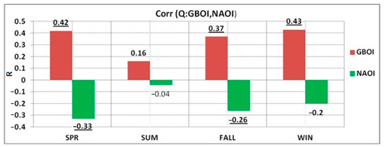
Figure 2.
The Pearson correlation coefficient (R), between the discharge of the Danube at Orsova (Q) and the climate indices GBOI and NAOI, considered simultaneously in the same season (1901–2000). The underlined values indicate a confidence level (CL) of 99% and those in bold indicate a 95% CL.
Regarding the influences of the two climatic indices, NAOI and GBOI, in the upper and middle basin of the Danube, their weight changes. In Mares et al. (2018) [27], the influence of the two indices on the precipitation of the entire Danube basin during the winter season was analyzed, and it was found that, for the upper basin and part of the middle basin, the NAOI is a predictor with a better statistical significance than the GBOI. This is in agreement with Lorenzo-Lacruz et al. [28], who showed that the NAOI is a good indicator for the processes in the upper Danube basin and for the European areas bordering the Atlantic Ocean.
As mentioned above, in addition to the two large-scale predictors, a regional-scale predictor was also considered, namely, the PHDI.
From our previous investigations, it emerged that the PHDI is a very good predictor for the discharge of the Danube at Orsova. The highest values of the correlation coefficients between Q and PHDI were found for the summer season and varied from 0.74 during the winter season to 0.86 during the summer (Figure 3).
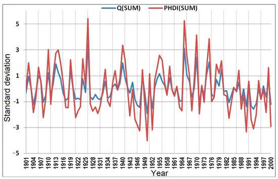
Figure 3.
The standardized values of the discharge at Orsova (Q) and of PHDI during the summer.
A complete image of the connections between the predictand (Q) and the four predictors for the summer season, obtained with a crossplot, is presented in Figure 4. In this case, the extra-atmospheric predictor, SSN, was taken as nonfiltered values.
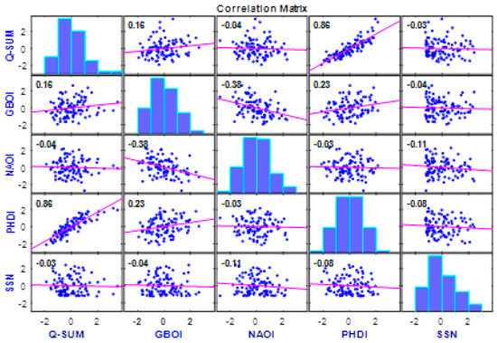
Figure 4.
Correlation matrix between the predictand (Q) and the four variables (GBOI, NAOI, PHDI and Wolf number (SSN)) for 1901–2000 during summer season.
2.2. Methods
The combination of mainly two methods is the essence of the study: (1) wavelet component analysis (filtering) and synthesis of the desired components and (2) prediction of the Danube discharge, following the “learning” analysis according to the predictors able to contribute to the evolution of Danube discharge.
A time series can be analyzed by its decomposition on several components according to two parameters: the dilation parameter, s > 0, and the translation parameter, u, . Such decomposition is performed through a real or complex function, , and called a wavelet, which is defined as follows:
The continuous wavelet transform (CWT) of the time series X(t) is defined by
and it helps us reconstruct the original series entirely. The * sign represents the complex conjugate of that expression.
In the present investigation, the Wolf number predictor was filtered by means of the continuous wavelet transform (CWT) [29,30,31]. In order to get the SSN signals related to 11-year (Schwabe) and to 22-year (Hale) solar cycles, the band pass filter with cut-off frequencies corresponding to periods of 9–15 years and, respectively, of 17–28 years, was used. All the time series were standardized, and all five predictors were orthonormalized to form a set of independent predictors.
In Figure 5, a perceptron is represented with an input layer, S0, which has the role of routing only; two hidden layers, Sx and Sy (circles), and the output layer, Sz. In Figure 5, the paths to the next layer Sx were drawn, only for the variable X1 and Xn. The arrows from X2 to X5 indicate similar routes as for X1 and Xn.
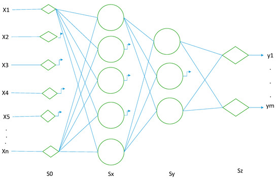
Figure 5.
A model of feed-forward neural network.
In the present study, we have the case of a network with a single hidden layer, with n = 5 (the number of variables) and a single predictand (m = 1).
The main property of the network is the forward propagation of the network signal only. Moreover, the network inputs used in this work are orthogonalized, and therefore, we do not have communications within the same layer.
The network assumes a training mechanism with the desired outputs. The “forward”-type networks with a single hidden layer and a single output of the linear regression type, with the activation function of the sigmoid type of the neurons, received an extremely favorable solution regarding the calculation speed (extreme learning machine—ELM) in the pioneering work of Huang [32] and Huang et al. [33]. Until then, neural networks with these characteristics were immense consumers of computing time. Since then, investigations have continued with more attention focused on the field of computational efficiency techniques [34,35,36,37,38,39,40].
The extremely fast computational model developed by Huang et al. [33] has inspired a lot of researchers who have developed it considerably, especially with regard to the propagation from one neuron to another in order to perform directed data transfer. The theoretical part was developed by Ribeiro et al. [39].
In the present paper, we used the MATLAB routines (https://github.com/vhrique/ELM (accessed on 2 June 2023)) provided by Ribeiro et al. [39], which follow the improved procedure of Huang et al. [33]. The procedure is summarized in Figure 6.
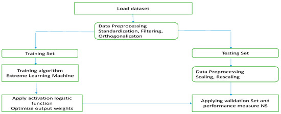
Figure 6.
Block diagram of the proposed study by neural network.
The performance measure of the results obtained by the ELM was taken as the Nash–Sutcliffe (NS) index [41] defined as
where is the ith observation, is ith estimated value by ELM in our case, is the mean of the observed data, and N is the total number of observations.
As shown in Pappenberger et al. [42], NS is a good evaluation in hydrological applications. In accordance with Moriasi et al. [43] and Alfieri et al. [44], the Nash–Sutcliffe index ranges between −∞ and 1.0. The value 1.0 is associated with optimal estimation. In general, the practical results can only be accepted if NS is greater than 0.5.
To our knowledge, for the first time, in the present investigation, a series of machine learning algorithms incorporating wavelet preprocessing of the input data for long-term (seasonal) prediction for distinct solar cycles were applied for a river in Europe, similar to research undertaken in Australia [36]. For the Danube basin, investigations on water quality were carried out by Mitrovic et al. using neural networks [45].
Machine learning is used to improve climate forecasts. As shown in [46], in machine learning with artificial intelligence systems, the performance improves with data accumulation, and machine learning techniques in climate science have a good performance.
The hybrid technique of combining “wavelet transform” with “deep learning” is not completely new; it has been used to predict runoff in rivers in Pakistan [47].
The experiments consisted of a simplified DL neural network [33] in which there is a single neural layer with no connections between the neurons of that layer, with a logistic activation function and an output in linear form. This simplified network architecture assumes that there is a “forward” propagation of the signal in the network as per terminology used by Dumitrescu and Hariton Costin [48].
3. Results and Discussions
In the present study, the “training” period was considered as the period 1901–1970, and the “validation” on independent data was performed for the period 1971–2000.
The forecasted series from the 30-year validation period, considering several combinations of predictors, as well as the series of observations of the Danube discharge at the Orsova station, during the time interval 1971–2000, are presented in Figure 7, Figure 8, Figure 9, Figure 10 and Figure 11. While, in Figure 7, Figure 8, Figure 9 and Figure 10, in addition to the geophysical predictors, the exogenous predictors from the filtered SSN series to highlight the Schwabe and Hale cycles are also introduced, in Figure 11, only the geophysical predictors are used to forecast the Danube discharge.
Figure 7 shows the experiment by which the extrapolation based on DL was carried out for the predictand, Q, with the GBOI predictor to which the SSN predictor, one of the two components corresponding to the Schwabe and Hale cycles at a time, was added. The prediction stands out through an almost coherent process. The predicted peaks under solar impact coincided with the observed peaks with the exception of peaks Nos. 2, 5 and 7. The prediction value according to the Nash–Sutcliffe index (NS) was unsatisfactory. The NS values were −0.7049 and −2.6440, for the Schwabe and Hale cycles, respectively.
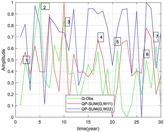
Figure 7.
The observed time series of the predictand (Q) for the interval 1971–2000 (green curve) compared to the predicted series, taking as predictors GBOI and SSN (Schwabe and Hale cycles, red and blue curves, respectively). All time series are scaled. 1, 2, 3, 4, 5, 6, 7—the peak numbers. (NS = −0.7049; −2.6440).
By considering the NAOI as a climate predictor and the SSN as an extra-atmospheric predictor, the predictand, Q, was computed, and the comparison with the observed one for the validation period is presented in Figure 8. The prediction under the impact of the NAOI and SSN in the form of the two cycles, was also carried out separately and led to a weak, unsatisfactory forecast according to the NS index, whose values were found to be −2.4567 and, −2.4063, respectively, in case of the solar cycle at the two considered timescales.
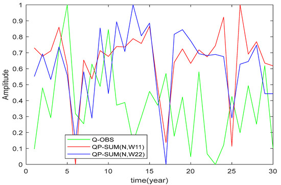
Figure 8.
Same as Figure 7, but with NAOI instead of GBOI (NS = −2.4567; −2.4063).
The prediction of the Danube discharge taking into account both the PHDI geophysical predictor and the SSN predictor is presented in Figure 9. It should be noticed that the observed peaks coincided with the forecasted ones due to the presence of both Schwabe and Hale solar activity cycles, with the exception of peak No. 3, where the forecasts were ahead of the observation area. The amplitude of the forecasted discharge under the impact of the PHDI and the Schwabe SSN was closer (visually) to that of the observational series. The NS index corresponding to the Hale cycle was higher than that for the Schwabe cycle, 0.7304 compared to 0.6542, and could be used to estimate the long-term discharge of the Danube.
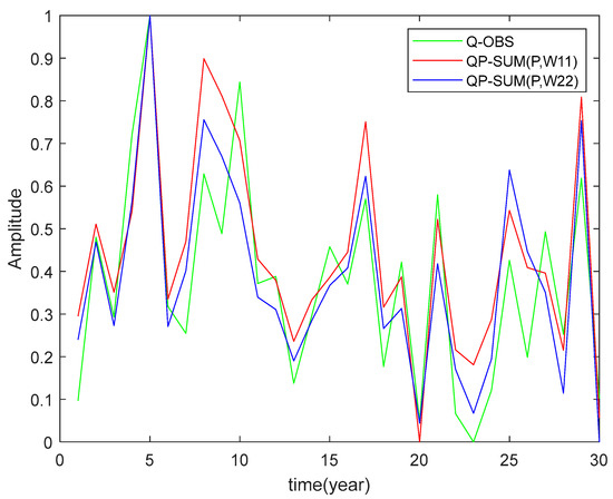
Figure 9.
Same as Figure 8, but with PHDI instead of NAOI (NS = 0.6542; 0.7304).
In Figure 10, all three endogenous predictors (GBOI, NAOI and PHDI) were considered, to which the exogenous ones were added, each in separate experiments. The best agreement can be noted, except for the third and sixth peaks, which were produced in advance compared to the observed peaks. But, in both cases of inconsistency, the advance was captured by a previously developed secondary peak. It can be mentioned that the amplitude of the peaks was also satisfactorily captured, having NS values of 0.6228 and 0.6913 for the two forecasted cases. Objectively, however, the NS index was a little lower compared to the previous experiment.
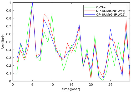
Figure 10.
Same as Figure 9, but instead of PHDI, the three terrestrial predictors are used (GBOI, NAOI, PHDI) (NS = 0.6228; 0.6913).
As mentioned at the beginning of this section, in the last experiment shown in Figure 11, the forecast of the Danube discharge at the Orsova station was performed based only on the set of endogenous predictors. It should be noted that, in general, all the important peaks (except for peak No. 3) existing in the evolution of the discharge, Q, during the 30-year validation period, were captured. The predicted amplitudes, for some peaks, differ substantially from the observed ones and the NS value of 0.4129 is much lower than that in the two previous experiments, when the exogenous predictors were taken into account.
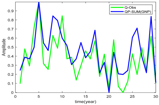
Figure 11.
The time series of the observed discharge (Q) (green curve) in comparison with the forecasted one (blue curve), considering only the three terrestrial predictors (GBOI, NAOI and PHDI) (NS = 0.4129).
The results presented in Figure 7, Figure 8, Figure 9, Figure 10 and Figure 11 could be explained by their similarity to the partial information decomposition presented by Timme and Lapish [49], regarding the partial decomposition of information from a set of predictors competing to predict a certain phenomenon. In the present case, all conditions were ensured for the set of predictors to act on the predictand factor synergistically and nonredundantly.
This study proves, once again, that the correlative links between solar activity and hydroclimates depend both on the spatiotemporal scale and on a multitude of climatic indices in which the solar activity signature is present [50].
In their recent publication, Utrabo-Carazo et al. [51], by applying wavelet power spectra to several climate parameters, found significant periodicities of about 11 years, especially in the Western Mediterranean Oscillation Index, periodicities that can be associated with signatures of solar activity.
In the present case, we noted the coupling of two oscillators (Schwabe and Hale) with different phases and frequencies whose convolution is reflected in the impact on hydrological phenomena by means of a set of modulators such as atmospheric ones (GBOI and NAOI) or those with water content (PHDI). The hydroclimatic evolution, including the discharge of the Danube River, achieved through the dynamic series under the solar impact, is nothing more than a particular case of the universal principle of Kuramoto [52] that governs natural systems [53,54].
As shown, the filtered SSN signal, corresponding to the Hale solar cycle timescale, in certain combinations with terrestrial predictors might be a good predictor for the long-term evolution of the Danube discharge in the lower basin. It leads us to think of the first investigations by Hale and Nicholson [55] in which the Hale cycle was called the magnetic SSN cycle due to the integrity of the polarity change inside the Sun as well as its intensity compared to the cycle of ~11 years. That is why we can advance the hypothesis that some geophysical processes, such as the flow of water from a river over wide areas like the Danube, can be linked to the large amounts of precipitation that can be produced from the highly developed convective cloud layers, of which there is no shortage during stormy activity. This stormy activity can be seen as a disturbing agent of the terrestrial magnetic field, which in turn is subject to changes under solar impact.
The discriminatory results of the two solar cycles, concerning the solar impact on the Danube discharge are assumed to be due to both the filtering applied to the Wolf time series and the orthogonalization of the predictors that eliminate redundancies, and thus, the synergy of the set of predictors improves the forecast. The elimination of redundancy [56] in synergistic multiple linkages gives added value to nonlinear statistical physics for information theory in coevolutionary systems. Also, global wavelet coherence analysis with different lags between the predictand (discharge) and the predictor (SSN) can provide significant useful information, as recently obtained in the paper [57].
4. Conclusions
The long-term seasonal (summer) prediction of the Danube discharge in the lower basin, during the time interval 1971–2000, based on a set of atmospheric (NAOI, GBOI, PHDI) and extra-atmospheric (SSN) predictors, by using a series of machine learning algorithms incorporating wavelet preprocessing, has been discussed.
It is worth noting that the SSN during the summer has a nonnegligible additional contribution only in combination with certain terrestrial predictors, such as the PHDI, and a combination of all three (GBOI, NAOI, PHDI), identifying a discrimination between the contribution of the two solar cycles at the Schwabe and Hale timescales. The SSN was considered separately to highlight the discrimination between the 11-year (Schwabe) solar cycle and the 22-year (Hale) solar cycle.
It was shown, based on the NS index, a performance measure of the results given by extreme learning machine, that
- (i)
- The forecast of the Danube discharge by considering the ensemble of the three terrestrial predictors is less significant than that obtained by taking into account both the atmospheric and extra-atmospheric predictors.
- (ii)
- In association with certain terrestrial predictors, for instance the PHDI, the contribution of the Hale cycle is more significant than the contribution of the Schwabe cycle to the estimation of the Danube discharge in the lower basin.
Investigations using the ELM method, regarding the lags of the predictor variables, especially those related to solar activity compared to observations, and possibly causal investigations, must be carried out in the future.
Author Contributions
Conceptualization, C.M.; investigation, C.M., V.D. and I.M.; methodology, C.M., I.M. and V.D.; writing—original draft preparation, C.M., V.D., I.M. and C.D.; supervision and validation C.D. All authors have read and agreed to the published version of the manuscript.
Funding
This research received no external funding.
Institutional Review Board Statement
Not applicable.
Informed Consent Statement
Not applicable.
Data Availability Statement
Not applicable.
Conflicts of Interest
The authors declare no conflict of interest.
References
- Tirabassi, G.; Sevilla-Escoboza, R.; Buldú, J.M.; Masoller, C. Inferring the connectivity of coupled oscillators from time-series statistical similarity analysis. Sci. Rep. 2015, 5, 10829. [Google Scholar] [CrossRef] [PubMed]
- Masson-Delmotte, V.; Zhai, P.; Pirani, A.; Connors, S.L.; Péan, C.; Berger, S.; Caud, N.; Chen, Y.; Goldfarb, L.; Gomis, M.I.; et al. (Eds.) IPCC, Climate Change 2021: The Physical Science Basis. In Contribution of Working Group I to the Sixth Assessment Report of 689 the Intergovernmental Panel on Climate Change; Cambridge University Press: Cambridge, UK; New York, NY, USA, 2021; Volume 692, p. 2391. [Google Scholar] [CrossRef]
- Sedlacek, J.; Sukhodolov, T.; Egorova, T.; Karagodin-Doyennel, A.; Rozanov, E. Future climate under CMIP6 solar activity scenarios. Earth Space Sci. 2023, 10, 002783. [Google Scholar] [CrossRef]
- Tupikina, L.; Rehfeld, K.; Molkenthin, N.; Stolbova, V.; Marwan, N.; Kurths, J. Characterizing the evolution of climate networks. Nonlinear Proc. Geophys. 2014, 21, 705–711. [Google Scholar] [CrossRef]
- Mares, C.; Dobrica, V.; Mares, I.; Demetrescu, C. Solar Signature in Climate Indices. Atmosphere 2022, 13, 1898. [Google Scholar] [CrossRef]
- Shannon, C.E. A mathematical theory of communication. Bell Syst. Tech. J. 1948, 27, 379–423. [Google Scholar] [CrossRef]
- Guiasu, S. Information Theory with Applications; McGraw-Hill Inc.: London, UK, 1977. [Google Scholar]
- Khan, S.; Ganguly, A.R.; Bandyopadhyay, S.; Saigal, S.; Erickson, D.J.; Protopopescu, V.; Ostrouchov, G. Nonlinear statistics reveals stronger ties between ENSO and the tropical hydrological cycle. Geophys. Res. Lett. 2006, 33, L24402. [Google Scholar] [CrossRef]
- Vu, T.M.; Mishra, A.K.; Konapala, G. Information Entropy Suggests Stronger Nonlinear Associations between Hydro-Meteorological Variables and ENSO. Entropy 2018, 20, 38. [Google Scholar] [CrossRef]
- Schultz, D.M.; Lynch, P. 100 years of L. F. Richardson’s Weather Prediction by Numerical Process. Mon. Wea. Rev. 2022, 150, 693–695. [Google Scholar] [CrossRef]
- Charney, J.G.; Fjørtoft, R.; Von Neumann, J. Numerical integration of the barotropic vorticity equation. Tellus 1950, 2, 237–254. [Google Scholar] [CrossRef]
- Fu, C.; James, A.L.; Wachowiak, M.P. Analyzing the combined influence of solar activity and El Niño on streamflow across southern Canada. Water Resour. Res. 2012, 48, W05507. [Google Scholar] [CrossRef]
- Dong, L.; Fu, C.; Liu, J.; Zhang, P. Combined Effects of Solar Activity and El Niño on Hydrologic Patterns in the Yoshino River Basin, Japan. Water Resour. Manag. 2018, 32, 2421. [Google Scholar] [CrossRef]
- Dobrica, V.; Demetrescu, C.; Mares, I.; Mares, C. Long-term evolution of the Lower Danube discharge and corresponding climate variations: Solar signature imprint. Theor. Appl. Climatol. 2018, 133, 985–996. [Google Scholar] [CrossRef]
- Mares, I.; Dobrica, V.; Mares, C.; Demetrescu, C. Assessing the solar variability signature in climate variables by information theory and wavelet coherence. Sci. Rep. 2021, 11, 11337. [Google Scholar] [CrossRef]
- Cubasch, U.; Voss, R.; Hegerl, G.C.; Waszkewitz, J.; Crowley, T.J. Simulation of the influence of solar radiation variations on the global climate with an ocean-atmosphere general circulation model. Clim. Dyn. 1997, 13, 757–767. [Google Scholar] [CrossRef]
- Hood, L.; Schimanke, S.; Spangehl, T.; Bal, S.; Cubasch, U. The surface climate response to 11-yr solar forcing during northern winter: Observational analyses and comparisons with GCM simulations. J. Clim. 2013, 26, 7489–7506. [Google Scholar] [CrossRef]
- Widmann, M. One-Dimensional CCA and SVD, and Their Relationship to Regression Maps. J. Clim. 2005, 18, 2785–2792. [Google Scholar] [CrossRef]
- Hunt, B.G. Nonlinear Influences—A Key to Short-Term Climatic Perturbations. J. Atmos. Sci. 1988, 45, 387–395. [Google Scholar] [CrossRef]
- Wen, G.; Cahalan, R.F.; Rind, D.; Jonas, J.; Pilewskie, P.; Dong, L.; Wu, D.L.; Krivova, N.A. Climate responses to SATIRE and SIM-based spectral solar forcing in a 3D atmosphere-ocean coupled GCM. Published by EDP Sciences. J. Space Weather Space Clim. 2017, 7, A11. [Google Scholar] [CrossRef][Green Version]
- Hsieh, W.W. Nonlinear multivariate and time series analysis by neural network methods. Rev. Geophys. 2004, 42, RG1003. [Google Scholar] [CrossRef]
- Hsieh, W.W. Nonlinear principal component analysis of noisy data. Neural Netw. 2007, 20, 434–443. [Google Scholar] [CrossRef][Green Version]
- Jenkner, J.; Hsieh, W.W.; Cannon, A.J. Seasonal Modulations of the Active MJO Cycle Characterized by Nonlinear Principal Component Analysis. Mon. Weather Rev. 2011, 139, 2259–2275. [Google Scholar] [CrossRef]
- Elbeltagi, A.; Nagy, A.; Mohammed, S.; Pande, C.; Kumar, M.; Bhat, S.A.; Zsembeli, J.; Huzsvai, L.; Tamás, J.; Kovács, E.; et al. Combination of Limited Meteorological Data for Predicting Reference Crop Evapotranspiration Using Artificial Neural Network Method. Agronomy 2022, 12, 516. [Google Scholar] [CrossRef]
- Mares, I.; Mares, C.; Mihailescu, M. Stochastic modeling of the connection between sea level pressure and discharge in the Danube lower basin by means of Hidden Markov Model. EGU Gen. Assem. Conf. Abstr. 2013, 15, 7606. [Google Scholar]
- Mares, I.; Mares, C.; Dobrica, V.; Demetrescu, C. Selection of Optimal Palmer Predictors for Increasing the Predictability of the Danube Discharge: New Findings Based on Information Theory and Partial Wavelet Coherence Analysis. Entropy 2022, 24, 1375. [Google Scholar] [CrossRef]
- Mares, I.; Mares, C.; Dobrica, V.; Demetrescu, C. Spectral coherence between precipitation in the Danube basin and indices of the teleconnections patterns by means of wavelet transform. Geophys. Res. Abstr. 2018, 20, 7562. Available online: https://meetingorganizer.copernicus.org/EGU2018/-7562.pdf (accessed on 2 June 2023).
- Lorenzo-Lacruz, J.; Morán-Tejeda, E.; Vicente-Serrano, S.M.; Hannaford, J.; García, C.; Peña-Angulo, D.; Murphy, C. Streamflow frequency changes across western Europe and interactions with North Atlantic atmospheric circulation patterns. Glob. Planet. Change 2022, 212, 103797. [Google Scholar] [CrossRef]
- Torrence, C.; Compo, G.P. A practical guide to wavelet analysis. Bull. Am. Meteorol. Soc. 1998, 79, 61–78. [Google Scholar] [CrossRef]
- Grinsted, A.; Moore, J.C.; Jevrejeva, S. Application of the cross wavelet transform and wavelet coherence to geophysical time series. Nonlin. Proc. Geophys. 2004, 11, 561–566. [Google Scholar] [CrossRef]
- Moore, J.; Grinsted, A.; Jevrejeva, S. Is there evidence for sunspot forcing of climate at multi-year and decadal periods? Geophys. Res. Lett. 2006, 33, L17705. [Google Scholar] [CrossRef]
- Huang, G.-B. Learning capability and storage capacity of two-hidden-layer feedforward networks. IEEE Trans. Neural Netw. 2003, 14, 274–281. [Google Scholar] [CrossRef]
- Huang, G.B.; Zhu, Q.Y.; Siew, C.K. Extreme learning machine: Theory and applications. Neurocomputing 2006, 70, 489–501. [Google Scholar] [CrossRef]
- He, Q.; Shang, T.; Zhuang, F.; Shi, Z. Parallel extreme learning machine for regression based on MapReduce. Neurocomputing 2013, 102, 52–58. [Google Scholar] [CrossRef]
- Antico, A.; Torres, M.E. Evidence of a decadal solar signal in the Amazon River: 1903 to 2013. Geophys. Res. Lett. 2015, 42, 782–787. [Google Scholar] [CrossRef]
- Deo, R.C.; Tiwari, M.K.; Adamowski, J.F.; Quilty, J.M. Forecasting effective drought index using a wavelet extreme learning machine (W-ELM) model. Stoch. Environ. Res. Risk Assess. 2017, 31, 1211–1240. [Google Scholar] [CrossRef]
- Bergout, T. A New Health Assessment Prediction Approach: Multi-Scale Ensemble Extreme Learning Machine. Preprints 2020, 2020050386. [Google Scholar] [CrossRef]
- Yaseen, Z.M.; Faris, H.; Al-Ansari, N. Hybridized Extreme Learning Machine Model with Salp Swarm Algorithm: A Novel Predictive Model for Hydrological Application. Complexity 2020, 2020, 8206245. [Google Scholar] [CrossRef]
- Ribeiro, V.H.A.; Reynoso, M.G.; Siqueira, H.V. Multi-Objective Ensembles of Echo State Networks and Extreme Learning Machines for Streamflow Series Forecasting. Eng. Appl. Artif. Intell. 2020, 95, 103910. [Google Scholar] [CrossRef]
- Khan, A.; Ali, A.; Islam, N.; Manzoor, S.; Zeb, H.; Azeem, M.; Ihtesham, S. Robust Extreme Learning Machine Using New Activation and Loss Functions Based on M-Estimation for Regression and Classification. Sci. Program. 2022, 2020, 6446080. [Google Scholar] [CrossRef]
- Nash, J.E.; Sutcliffe, J.V. River flow forecasting through conceptual models part I—A discussion of principles. J. Hydrol. 1970, 10, 282–290. [Google Scholar] [CrossRef]
- Pappenberger, F.; Scipal, K.; Buizza, R. Hydrological aspects of meteorological verification. Atmos. Sci. Lett. 2008, 9, 43–52. [Google Scholar] [CrossRef]
- Moriasi, D.N.; Arnold, J.G.; Van Liew, M.W.; Bingner, R.L.; Harmel, R.D.; Veith, T.L. Model evaluation guidelines for systematic quantification of accuracy in watershed simulations. Trans. ASABE 2007, 50, 885–900. [Google Scholar] [CrossRef]
- Alfieri, L.; Pappenberger, F.; Wetterhall, F.; Haiden, T.; Richardson, D.; Salamon, P. Evaluation of ensemble streamflow predictions in Europe. J. Hydrol. 2014, 517, 913–922. [Google Scholar] [CrossRef]
- Mitrović, T.; Antanasijević, D.; Lazović, S.; Perić-Grujić, A.; Ristić, M. Virtual water quality monitoring at inactive monitoring sites using Monte Carlo optimized artificial neural networks: A case study of Danube River (Serbia). Sci. Total Environ. 2019, 654, 1000–1009. [Google Scholar] [CrossRef] [PubMed]
- Jones, N. How machine learning could help to improve climate forecasts. Nature 2017, 548, 379. [Google Scholar] [CrossRef] [PubMed]
- Pandhiani, S.; Shabri, A. Time Series Forecasting Using Wavelet-Least Squares Support Vector Machines and Wavelet Regression Models for Monthly Stream Flow Data. Open J. Statist. 2013, 3, 183–194. [Google Scholar] [CrossRef]
- Dumitrescu, D.; Costin, H. Inteligenta artificiala. In Retele Neuronale-Teorie si Aplicatii; Brosate: Bucuresti, Romania, 1996; p. 45. [Google Scholar]
- Timme, N.M.; Lapish, C. A tutorial for information theory in neuroscience. eNeuro 2018, 5, ENEURO.0052-18.2018. [Google Scholar] [CrossRef] [PubMed]
- Le Mouël, J.L.; Lopes, F.; Courtillot, V. A solar signature in many climate indices. J. Geophys. Res. Atmos. 2019, 124, 2600–2619. [Google Scholar] [CrossRef]
- Utrabo-Carazo, E.; Azorin-Molina, C.; Aguilar, E.; Brunet, M. A spectral analysis of near-surface mean wind speed and gusts over the Iberian Peninsula. Geophys. Res. Lett. 2023, 50, e2023GL103323. [Google Scholar] [CrossRef]
- Kuramoto, Y. Chemical Oscillations, Waves, and Turbulence; Courier Dover Publications: Mineola, NY, USA, 2003. [Google Scholar]
- Kabir, M.; Stan, M. Computing with hybrid CMOS/STO circuits. In Proceedings of the 51st Annual Design Automation Conference, San Francisco, CA, USA, 1–5 June 2014; pp. 1–6. [Google Scholar]
- Pikovsky, A.; Rosenblum, M.; Kurths, J. Synchronization, a Universal Concept in Nonlinear Sciences; Cambridge University Press: Cambridge, MA, USA, 2003. [Google Scholar]
- Hale, G.E.; Nicholson, S.B. The law of sun-spot polarity. Astrophys. J. 1925, 62, 270. [Google Scholar] [CrossRef]
- Perdigão, R.A.P. Polyadic Entropy, Synergy and Redundancy among Statistically Independent Processes in Nonlinear Statistical Physics with Microphysical Codependence. Entropy 2018, 20, 26. [Google Scholar] [CrossRef]
- Wrzesiński, D.; Sobkowiak, L.; Mares, I.; Dobrica, V.; Mares, C. Variability of River Runoff in Poland and Its Connection to Solar Variability. Atmosphere 2023, 14, 1184. [Google Scholar] [CrossRef]
Disclaimer/Publisher’s Note: The statements, opinions and data contained in all publications are solely those of the individual author(s) and contributor(s) and not of MDPI and/or the editor(s). MDPI and/or the editor(s) disclaim responsibility for any injury to people or property resulting from any ideas, methods, instructions or products referred to in the content. |
© 2023 by the authors. Licensee MDPI, Basel, Switzerland. This article is an open access article distributed under the terms and conditions of the Creative Commons Attribution (CC BY) license (https://creativecommons.org/licenses/by/4.0/).