Article

Hour-by-Hour Prediction Model of Air Pollutant Concentration Based on EIDW-Informer—A Case Study of Taiyuan

1
School of Environmental and Chemical Engineering, Shanghai University, Shanghai 200444, China
2
School of Computer Engineering and Science, Shanghai University, Shanghai 200444, China
*
Author to whom correspondence should be addressed.
Atmosphere 2023, 14(8), 1274; https://doi.org/10.3390/atmos14081274
Submission received: 12 June 2023 / Revised: 7 August 2023 / Accepted: 8 August 2023 / Published: 11 August 2023
(This article belongs to the Section Atmospheric Techniques, Instruments, and Modeling)

Abstract

:
Prediction of air pollutant concentrations is currently one of the most important methods for the prevention and control of urban air pollution in most countries, and accurate and timely prediction of pollutant concentrations is of great significance for urban pollution control. Using Taiyuan, China, as a case study, this study examines how to predict hourly air pollutant concentrations over longer periods of time while ensuring their accuracy. In this paper, an air pollutant concentration prediction method based on improved inverse distance interpolation and Informer model (EIDW-Informer), and hour-by-hour prediction of PM2.5, NO2, and O3 concentrations in Taiyuan, China is carried out. In this study, historical data from seven environmental monitoring stations in Taiyuan City were used to build multidimensional environmental vectors and calculate the similarity between sample points. Then, the missing values in the dataset were interpolated according to the similarity and distance weights, and the long series prediction was performed by Informer. The experimental results show that the EIDW-Informer method has advantages in hour-by-hour prediction compared to LSTM, CNN-LSTM, and Attention-LSTM models, which improves by 20%, 27%, and 43% on 1 h, 8 h, and 72 h time scales, respectively.

1. Introduction

1.1. Background

According to the definition made by the International Organization for Standardization (ISO), air pollution, also known as atmospheric pollution, generally refers to the phenomenon where certain substances are introduced into the atmosphere due to human activities or natural processes, presenting a sufficient concentration and duration to harm human comfort, health, or the environment.
In 2013, the WHO and the International Agency for Research on Cancer (IARC) issued a report identifying air pollution as a human Group I carcinogen. In 2016, the World Health Organization (WHO) estimated that outdoor air pollution exposure causes 4.2 million deaths in people each year [1]. The Global Burden of Disease Study states that in 2015 China had 1.108 million premature deaths and 21.779 million disability-adjusted life years due to outdoor PM2.5 pollution, ranking fourth and fifth per 100,000 of the world’s 10 most populous countries. Furthermore, the number of global deaths caused by outdoor particulate pollution increased from 3.5 million in 1990 to 4.2 million in 2015 [2]. According to data from the 2019 China Ecological Environment Status Bulletin, only 158 of the country’s 338 cities at the prefecture level and above met ambient air quality standards, with 53.4% of cities failing to meet air quality standards. Every year, more than 350,000 people die in China due to air pollution, and more than a third of the population lives in an air-polluted environment for long periods of time [3,4]. On 22 September 2021, WHO released updated guidelines for global air quality. The guidelines recommend limits for concentrations of several key pollutants (including PM2.5, PM10, O3, NO2, SO2, and CO) alongside a new set of interim targets [5]. At the same time, a series of policies adopted by various countries to deal with air pollution have also achieved certain results [6]. Therefore, comprehensive, scientific, and accurate analysis and prediction of air quality are of great significance to the public in avoiding health damage caused by air pollution and guiding governmental agencies in formulating relevant policies.

1.2. Literature Review

When predicting air quality, the question of how to ensure both the prediction of air quality over a long period of time and the accuracy of the prediction has been an ongoing concern for many researchers. Researchers typically use ground-based observations supplemented by remote sensing or meteorological data for their studies. Castell et al. [7] evaluated the performance of a commercially available low-cost sensor (AQMesh v3.5) for the measurement of four gaseous pollutants (NO, NO2, O3, and CO) and particulate matter (PM10 and PM2.5), illustrating its limitations. Lin et al. [8] developed a method for estimating long-term PM2.5 concentrations by combining satellite remote sensing technology and a network of low-cost sensors without reference to ground-based PM2.5 observations. An observation-based method to estimate long-term PM2.5 concentrations. Van Donkelaar et al. [9] derived estimates of global fine particulate matter (PM2.5) concentrations by applying global geographically weighted regression (GWR) to geophysically-based satellite-derived PM2.5 concentration estimates using satellite, modeling, and monitoring data. Motlagh et al. [10] develop a vision of massive-scale air quality monitoring that delivers accurate air quality information at high spatial and temporal resolution. Prediction of air pollutant concentrations based on ground-based observations is required. Whether statistical or machine learning methods are used, more accurate and detailed observations are effective in improving the accuracy of predictions.
In past research, statistical and machine learning methods have been the two main types of forecasting methods. Statistical methods predict air quality by applying statistically based models. To accommodate time series prediction problems with non-stationary input data such as air quality prediction, Box et al. [11]. Proposed the Autoregressive Integrated Moving Average model (ARIMA), which has a significant advantage in this model is that it solves the problem of converting non-stationary data into stationary data and improves the forecasting capability of the model. Jian et al. [12] applied ARIMA to the prediction of PM10 concentrations in Hangzhou and proposed a framework for predicting the effect of meteorological factors on the concentration of submicron particles in the air. Williams et al. [13] added the effect of seasonal components to the ARIMA model and proposed a SARIMA model, which was used to predict univariate traffic data streams, and Voynikova et al. [14] used the SARIMA model to predict SO2 and PM10 concentrations in Bulgaria, demonstrating the feasibility of using the model for air quality prediction. However, most of the studies did not change the basic structure of the moving average autoregressive model but processed the inputs of the model or used the model in combination with other models. Although better results were achieved, the disadvantage of the moving average autoregressive model itself, which is based on the assumption of linearity, still exists, and the parameters of the model are not well determined, so there is still a large room for improvement in the method.
In terms of shallow machine learning, a variant of the support vector machine model, the support vector regression model (SVR), is often used for the task of time series prediction. Wang et al. [15] compared the support vector regression model with a Back Propagation neural network(BP) for PM2.5 prediction and analyzed that the support vector regression model was superior to the BP in air quality prediction. Lijie Dai et al. [16] proposed an air quality prediction model fusing support vector machine and particle swarm algorithm to predict PM2.5 in Shanghai for 24 h. However, the support vector machine model seriously affects its prediction performance due to the problem of high computational complexity and excessive computational effort when facing massive data.
In deep learning, to cope with the problem of gradient disappearance and gradient explosion when the sequence of input neural networks is too long in convolutional neural networks (CNN) [17], Hochreiter and Schmidhuber proposed a long- and short-term memory network(LSTM) [18], which proposes a structure called a gating cell that allows the network to have a “memory” that is propagated in the form of cellular states. In 2017, Li et al. [19] used LSTM to predict PM2.5 concentrations in Beijing and showed that LSTM outperformed other models, such as ARIMA and SVR. In 2018, Wen et al. [20] incorporated data from proximity air monitoring sites and meteorological data into the model through a combination of CNN and LSTM. In 2019, Ma et al. [21] combined migration learning and LSTM to predict air quality at new sites to cope with the shortcomings of insufficient historical data at new sites. In 2020, Liu et al. [22] came up with a novel wind-sensitive attention mechanism that uses LSTM neural network models to predict future PM2.5 concentrations by considering the effects of wind direction and wind speed on the spatial and temporal variation of PM2.5 concentrations in neighboring areas. However, most of the existing methods are designed based on short-term problems, and the long time-series prediction problem (LSTF) can strain the predictive power of existing models.
The Transform model proposed by Vaswani et al. [23] in 2017 shows excellent performance in capturing long-range dependency, and the self-attention mechanism proposed by the model shortens the element-to-element distance from the CNN logarithmic path length to constant path length, which shows great potential in handling LSTF problems. However, Transform models are currently often deployed on dozens of GPUs for training, and long time-series prediction problems such as air quality prediction cannot afford such costs. At the same time, Transform models require a large amount of continuous historical data for training. In hour-by-hour air monitoring station monitoring data, there are often missing data due to damage, maintenance, and updates to the station hardware and software equipment, and such data often do not meet the requirements of the Transform model input data, and suitable interpolation methods need to be used to interpolate the missing data.

1.3. Our Contribution

This paper proposes an air quality prediction method based on the Environmental Similarity Improved Inverse Distance Weighted Interpolation and Informer Model (EIDW-Informer) [24]. The proposed model is studied using hour-by-hour air quality data and meteorological data from 1 January 2018 to 31 October 2021 at seven environmental monitoring stations in Taiyuan City. The main contributions of this paper are as follows:
  • For the first time, the environmental similarity and inverse distance weighted interpolation methods were combined to create a multi-dimensional environmental vector of historical air pollutant concentration data and meteorological data from seven environmental monitoring stations in the urban area of Taiyuan City, from which the environmental similarity between sample points was calculated, and then the missing data in the dataset were interpolated according to the combined weight of the environmental similarity and relative distance of each sample point, in order to solve the missing data problem faced in air quality prediction.
  • In this study, a Transformer-based Informer model was selected to solve the problem of air quality prediction. Compared with the original model, the prediction effect of the EIDW-Informer model increased by 20%, 27%, and 43% in three time scales of 1 h, 8 h, and 72 h, respectively, and the model achieved a good balance in terms of training cost and prediction effect.

1.4. Dataset

The datasets used in this study were hourly air quality data and meteorological data from 1 January 2018 to 31 October 2021 at seven monitoring stations in the urban area of Taiyuan City, as shown in Figure 1. The data used in this study are all local monitoring station monitoring data. Air pollutant concentrations data were obtained from the China National Environmental Monitoring Centre (http://www.cnemc.cn (accessed on 10 February 2022)) and meteorological data were obtained from The National Data Center for Meteorological Sciences (http://www.nmic.cn/ (accessed on 10 February 2022)). In this paper, three major air pollutants, PM2.5, NO2, and O3, were selected as the prediction targets. The hourly pollutant concentrations were predicted for the next 1, 8, and 72 h, respectively, in order to test the hourly prediction effect of the model for different time periods. Among the whole dataset, the data from January 2018 to December 2020 were used for training, and the data from January to October 2021 were used for testing.

2. EIDW Method

2.1. Interpolation Methods

IDW was proposed by Donald Shepard in 1968 [25]. The method is based on the idea that the attributes of points that are closer together will be more similar: The attribute value of an unsampled point is calculated as the weighted average of known values within its neighborhood, where the weights are inversely proportional to the distances between the prediction location and the sampled locations. This method can produce deterministic and continuous interpolation results quickly, but it is strongly influenced by the choice of the weight function, and the interpolated points are prone to clumping, where similar sample points contribute almost the same amount to the interpolated point, and the eigenvalues of the point to be interpolated are significantly higher than those of the surrounding samples [26]. Lu et al. [27], in 2008, proposed an adaptive IDW spatial interpolation technique whose weight parameters can vary according to the spatial patterns of the sampled points in the critical domain. Zhu et al. 2015 [28] considered the influence of environmental similarity on the spatial interpolation results in soil mapping. Lotrecchiano et al. 2021 [29] took into account factors such as wind direction and wind strength when using IDW to interpolate air quality data and achieved good results. Therefore, in addition to the distance factor, the distribution of pollutant concentrations in urban areas is also related to various factors such as geography, industrial distribution, and meteorological conditions [30]. We propose a new spatial interpolation method (EIDW) for air quality data based on IDW and taking into account the influence of environmental similarity.

2.2. Environmental Similarity

The concept of environmental similarity was proposed by the third law of geography, the basic idea of which is that locations with similar environmental attributes tend to have similar values of the attributes to be studied. Combined with the study by Zheng et al. [31], data including various types of environmental pollutants affecting air quality, such as PM2.5, PM10, SO2, CO2, NO2, O3 data collected by air quality monitoring stations, and relative humidity, wind speed, wind direction data as environmental vectors for constructing environmental attribute configurations.
We construct the environmental data selected above as an m-dimensional environmental vector and denote it by e. For any of the points to be predicted and the sample points in the study area, we can construct an m-dimensional environmental vector shaped as follows:
e = ( e 1 , e 2 , , e i , , e m )
where e denotes the environment vector, m denotes the dimensionality of the environment vector, and e i denotes the attribute value of the i-th feature of the environment vector. Next, for each point to be predicted, the similarity between it and each sample point is calculated as follows:
S i , j = P ( E ( e i 1 , e j 1 ) , E ( e i 2 , e j 2 ) , , E ( e i v , e j v ) , , E ( e i m , e j m )
where S i , j , which is the environmental similarity between the location i to be speculated and the sample location j. e i v with e j v (v = 1,2,…, m) is the attribute value of the v-th dimension of the environment vector at locations i and j, and the function E ( ) is a function to calculate the environmental similarity between the point to be predicted and the individual feature of the sample point, e i v . e j v . with, and the function P ( ) is a function to calculate the overall similarity between points i and j.
where:
E ( e i v , e j v ) = e x p ( e i v e j v ) 2 2 ( S D e v S D e v S D e j v ) 2
The function E ( e i v , e j v ) represents the similarity of environmental attributes between point i to be predicted and sample point j in the v-th dimension, where S D e v is the standard deviation of the environmental configuration of the v-th attribute in the study area, and S D e j v is the square root of the mean deviation of all the locations(i = 1,2,…,k; k is the number of locations to be predicted) to be predicted, which is calculated as shown below:
S D e j v = i = 1 k ( e i v e j v ) 2 k
In this paper, the weighted average method was used to S i , j . The solution was carried out with the following equation:
S i , j = a E ( e i 1 , e j 1 ) + b E ( e i 2 , e j 2 ) + + n E ( e i m , e j m ) a + b + + n
where a, b, …, n are the weights of each environmental factor. By solving for the function P ( ) , we obtain the environmental similarity between the point i to be predicted and all sample points, so for each point i to be predicted, an environmental similarity vector can be obtained S i , j that is shown in equation:
S i = ( S i , 1 , S i , 2 , , S i , k , , S i , n )
where S i , k is the similarity between the point i to be predicted and the sample point k on the scale of environmental variables.
This leads us to the EIDW spatial interpolation method, which proceeds as follows:
Z ^ ( P i ) = j = 1 n λ j Z ( P j )
λ j = S i , j d i , j α j S i , j d i , j α
In the above equation Z ^ ( P i ) is the attribute value of the point to be predicted, and Z ( P j ) is the data for a single sample point, and λ j is the weighting factor.
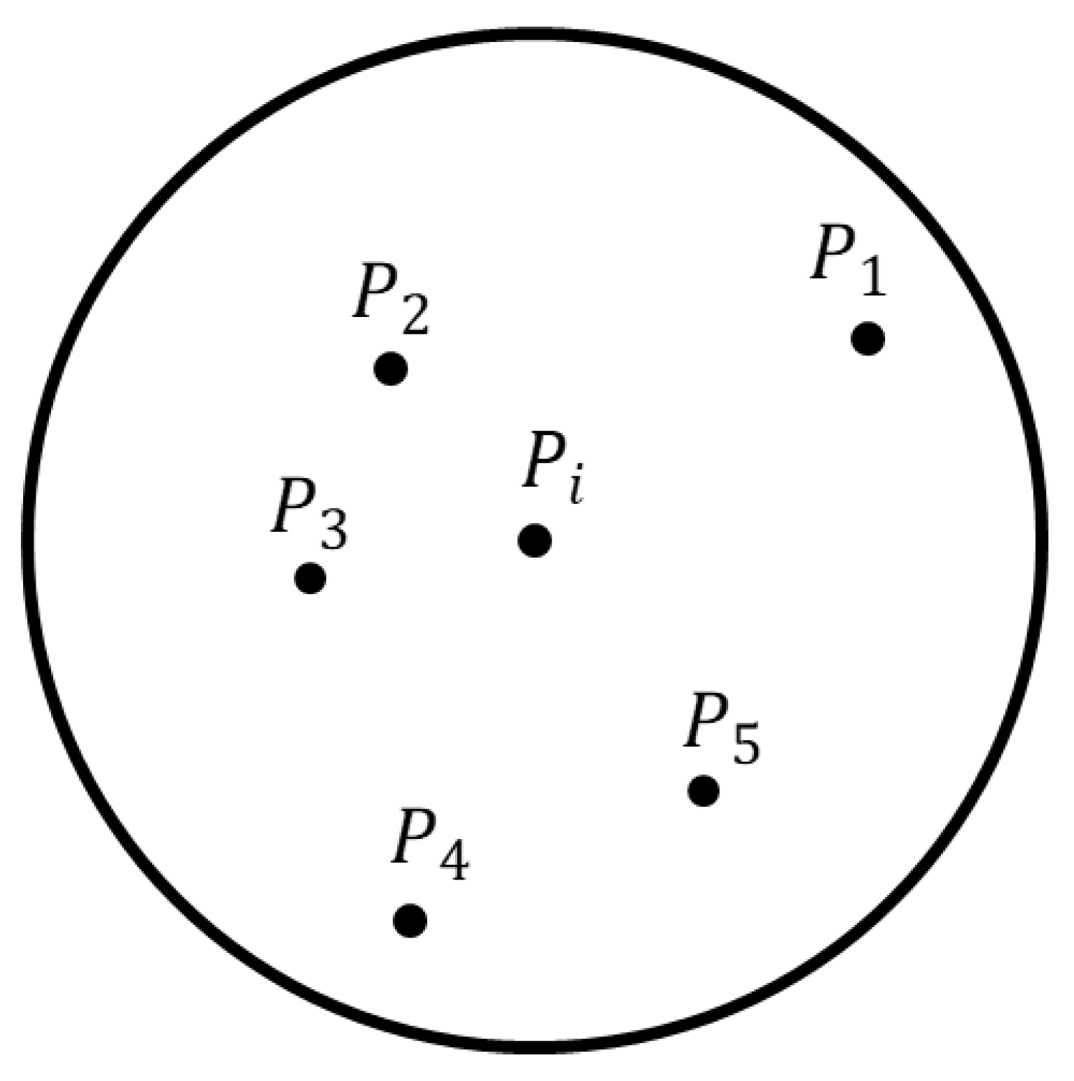
As shown in Figure 2, assume that the location of the point to be interpolated is P i , the position of the sample point is P j , the distance between the sample point i and the point j to be predicted is d i , j , in order to obtain smoother results, this study uses the distance inverse ratio leveling method to set the value of α to 2.

2.3. Interpolation Method Verification

2.3.1. Correlation Analysis

According to the previous section, hour-by-hour air quality data from seven air monitoring stations in Taiyuan from 1 January 2018 to 31 October 2021 were used for this study. Air quality data were obtained from the China National Environmental Monitoring Centre (http://www.cnemc.cn (accessed on 10 February 2022)). The numbers and physical locations of these air quality monitoring stations are shown in Figure 1.
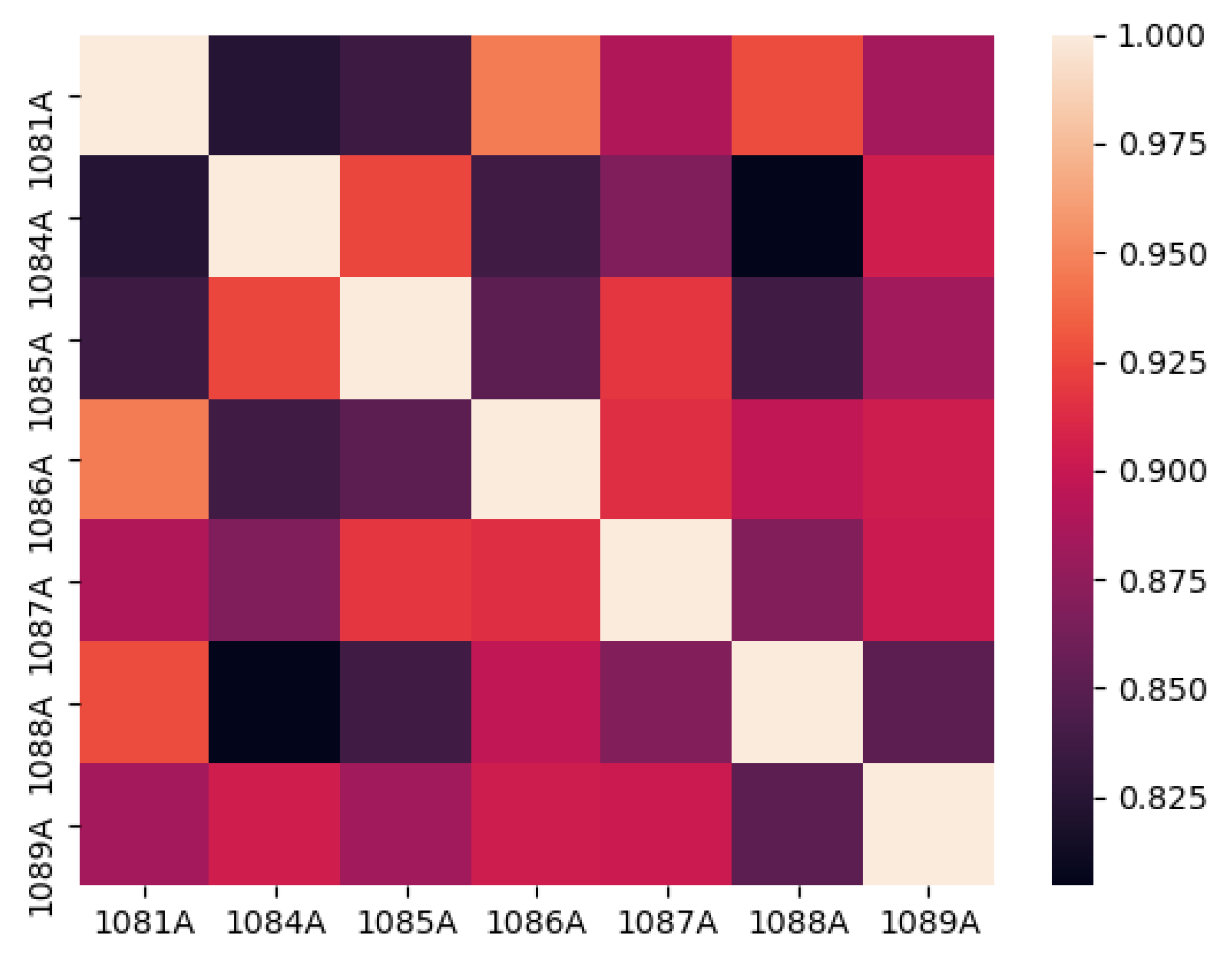
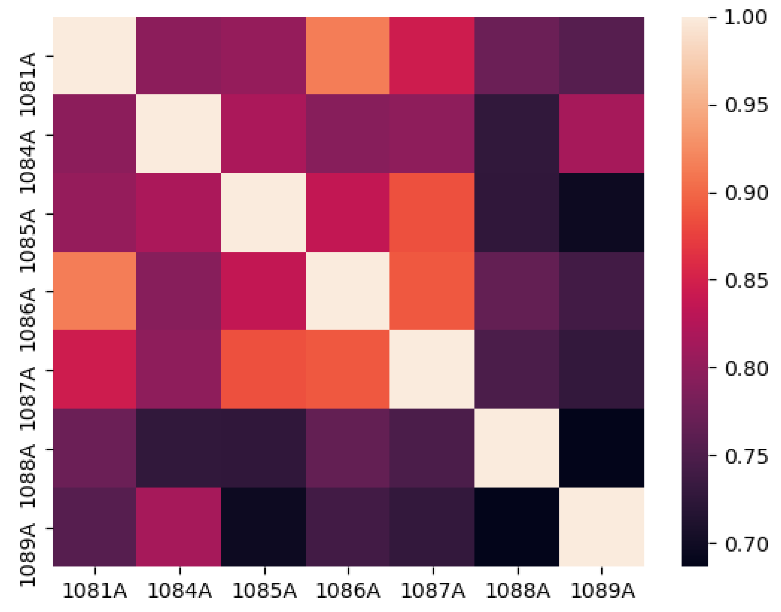
In this paper, the Pearson coefficient metric was used as a measure of spatial autocorrelation to test the correlation of each of these seven monitoring stations, and the results obtained are shown in Figure 3, Figure 4 and Figure 5.
The correlation results show that the correlations between the various air monitoring stations are high and generally conform to the guideline that the closer the station, the higher the correlation, except for two obvious problems. One is the close proximity but low PM2.5 correlation between stations 1081 A and 1084 A. One of the possible reasons for this is the building distribution factor, as can be seen from the HD satellite map, which shows that there are a number of continuous high-rise buildings to the north of 1084 A, which may lead to the aggregation of fine particulate pollutants at this station due to the building distribution. The second is that 1088 A and 1089 A are both low in NO2 correlation with other sites, where 1088 A is relatively far away from other sites, while 1089 A may be influenced by topography and wind direction, Taiyuan is influenced by northwest wind most of the year [32], while northwest of 1089 A is a high altitude mountain range, so air pollutants at site 1089 A are not easily move by northwesterly winds and the correlation with other stations is low. Meanwhile, the results of the correlation test show that the concentration distribution of O3 is mainly determined by distance, and factors such as topography, wind direction, and building distribution have little influence on it; this may be caused by the spatial distribution of O3 in the atmosphere at higher distances from the surface [33].

2.3.2. Evaluation Indicators

In order to verify the validity of the interpolation method, this experiment used air quality data from random monitoring stations in different seasons as the validation set, random masking of 15% of the data in the validation set, by interpolating PM2.5, NO2, and O3 data using EIDW and IDW interpolation methods, respectively, and applying comparative experiments to determine the validity of the EIDW interpolation method studied in this paper. Metrics to evaluate the effectiveness of the interpolation method and the MAE and RMSE were calculated as follows:
MAE = 1 n i = 1 n | O i P i |
RMSE = 1 n i = 1 n ( O i P i ) 2
O i is the observed value of the sample, and P i is the predicted value of the sample, and n is the number of missing values. The lower the values of mean absolute error (MAE) and root mean square error (RMSE) of the experimental results, the smaller the error of the interpolation results and the more effective the spatial interpolation method is. The experimental results are shown in Table 1:
The experimental results show that the comparison of the mean absolute error and the root mean square error when applying the two methods to PM2.5, NO2, and O3 concentration data are IDW > EIDW. The experimental results show that the EIDW interpolation method is more effective than the IDW method in interpolating the concentration data of three atmospheric pollutants, PM2.5, NO2, O3, by 11%, 19%, 6%, respectively. The reason for this is mainly due to the fact that the use of IDW interpolation only considers distance as the only metric to be considered. This scheme works well when there is a strong correlation with distance. Still, it is clear that air quality data are not only spatially correlated with distance but also strongly correlated with data such as wind direction, topography, and building distribution. Therefore, this study uses an EIDW-based interpolation method to complete the interpolation of air quality data for the study area, which can improve the prediction accuracy of the model.

3. Prediction Methodology

3.1. Prediction Model

Since Google proposed the Transformer model in 2017, it has achieved extremely good performance in computer vision (CV), natural language processing (NLP), etc. self-attention is the core of the Transformer, which uses Scaled Dot Product Attention to compute the degree of association, as shown in the flow with the following equation:
A t t e n t i o n ( Q , K , V ) = Softmax ( Q K T d k )
where Q represents the query feature matrix, K represents the key feature matrix, V represents the value feature matrix, Transformer encodes the input data into a multi-dimensional vector, the specific values of Q ,   K ,   V are obtained by transforming the input data, d k represents the dimensionality of Q ,   K ,   V ,   T is the transpose symbol, Softmax is the activation function, and A t t e n t i o n ( Q , K , V ) is the calculation process of self-attention. The formula calculates the similarity between the two based on Q and K, then normalizes the similarity, and finally, the output is obtained by weighting and summing V according to the similarity.
Based on Scaled Dot Product Attention, Transformer proposes Multi-Head Attention, which divides Q , K , V into h parts after transformation, and then performs Scaled Dot Product Attention calculation for each part separately. The formula for the multi-head self-attentive mechanism is shown in equations:
M u l t i H e a d ( Q , K , V ) = C o n c a t ( h e a d 1 , h e a d 2 , , h e a d h ) W 0
h e a d 1 = A t t e n t i o n ( Q W i Q , K W i K , V W i V )
where W i Q , W i K , W i V represents the parameter matrix of the i-th head, i takes values in the range [1, h], C o n c a t represents the stitching of each head, W 0 is the parameter matrix used for output. With Multi-Head Attention, the Transformer can learn information about different subspaces.
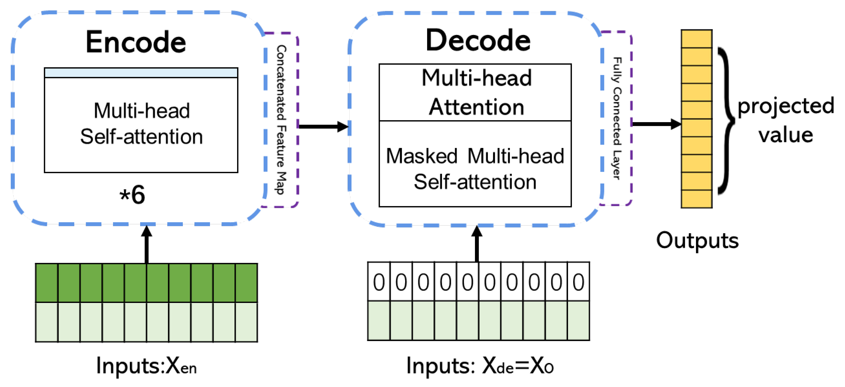
The model structure of the Transformer is shown in Figure 6; the Encoder and Decoder of the Transformer are a nest of six fixed structures. Each Encoder, Decoder contains two parts, (1) Multi-Head Attention plus residual linkage [34] and (2) Feedforward Neural Network [35] plus residual linkage.
Although the Transformer has shown its powerful modeling capability for sequence data, it has not performed well in the face of long sequence prediction problems, with three main shortcomings: firstly, the computational bottleneck, where the point-by-point computation of Self-Attention leads to time complexity of the square of the input sequence length L; secondly, the memory bottleneck, where the memory usage of the Transformer’s h-layer encoder and the memory usage of the decoder stack is O ( h L 2 ) , which limits the model’s ability to handle long sequence inputs; third, the speed bottleneck, the autoregressive nature of the Transformer’s decoding, the result of regression prediction at one moment depends on the result of the previous moment’s output, and this dynamic decoding approach limits the speed of long sequence regression prediction. To solve the above problems, in 2019, Li et al. [36] proposed ConvTrans, which enhances the focus on local contextual information through Convolutional Self-Attention and compensates for the high computational complexity of self-attention through LogSparse. In 2022 Zhou T [37] conducted a study on frequency domain modeling of time series data and processed attention operations in the frequency domain with Fourier transform and wavelet transform to reduce the computational effort to linear complexity while reducing noise.
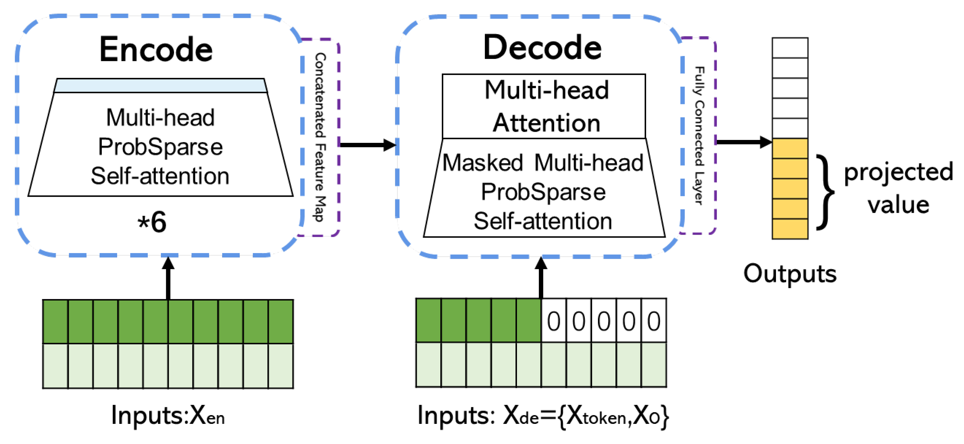
Figure 7 shows the model structure of Informer used in this paper. Informer addresses the shortcomings of the Transformer model in dealing with time series problems by decomposing the temporal features of the input data into quarterly, monthly, weekly, and daily features, focusing on the periodicity of the time-series data; the ProbSparse self-attention mechanism is proposed, according to the sparsity of the self-attention to the sparsity of the distribution of the weight scores, so that each Key vector only needs to pay attention to a limited number of Query vectors. Each layer of the Encoder and Decoder structure does a self-attention distilling. This reduces the model space and time complexity to O ( L log L ) . For example, if we need to predict the data for the next 8 h, we use the last 16 h of the encoder as the start token of the decoder and the 8 h of data to be predicted as the last 16 h of the encoder are used as the start token of the decoder, and the 8 h of predicted data are used as the end token, making up a 24-token input to the decoder, thus solving the problem of dynamic decoding of the decoder taking up a lot of time. With these improvements, Informer has successfully improved the accuracy of LSTF while significantly reducing the training cost of the model.

3.2. Predictive Performance Evaluation

After applying the EIDW method to the initial data set for interpolation, we conducted a series of comparison experiments to determine the model parameters, setting the learning rate to 0.0001, epochs to 6, batch size to 32, and the encode token and decode token to (168,4), (168,24), (168,168) for 1 h, 8 h, and 72 h, respectively, and then apply the Informer network model to model the data and predict the future air pollutant concentrations for 1 h, 8 h, and 72 h. Taking station 1081 A as an example, the data from January 2018 to December 2020 were used for training, and the data from January to October 2021 were used for testing. The prediction of air pollutant concentrations is a typical autoregressive problem; autoregression refers to the use of the historical time series of the prediction target in different periods of time between the values of the existence of the dependence relationship (i.e., its own correlation), through the past history of the target data to predict the value of the future period of time. The combined performance of each model can be effectively evaluated by statistical-based regression analysis metrics. Therefore, this paper also uses two classical evaluation metrics, mean absolute error (MAE) and root mean square error (RMSE), to evaluate the performance of each model. The lower the value of the mean absolute error (MAE) and root mean square error (RMSE) of the test results, the higher the prediction accuracy and the better the model performance.
The performance of the Informer model in predicting the three major air pollutants PM2.5, NO2, and O3 at three time levels of 1 h, 8 h, and 72 h for 1081 A is shown in Table 2.
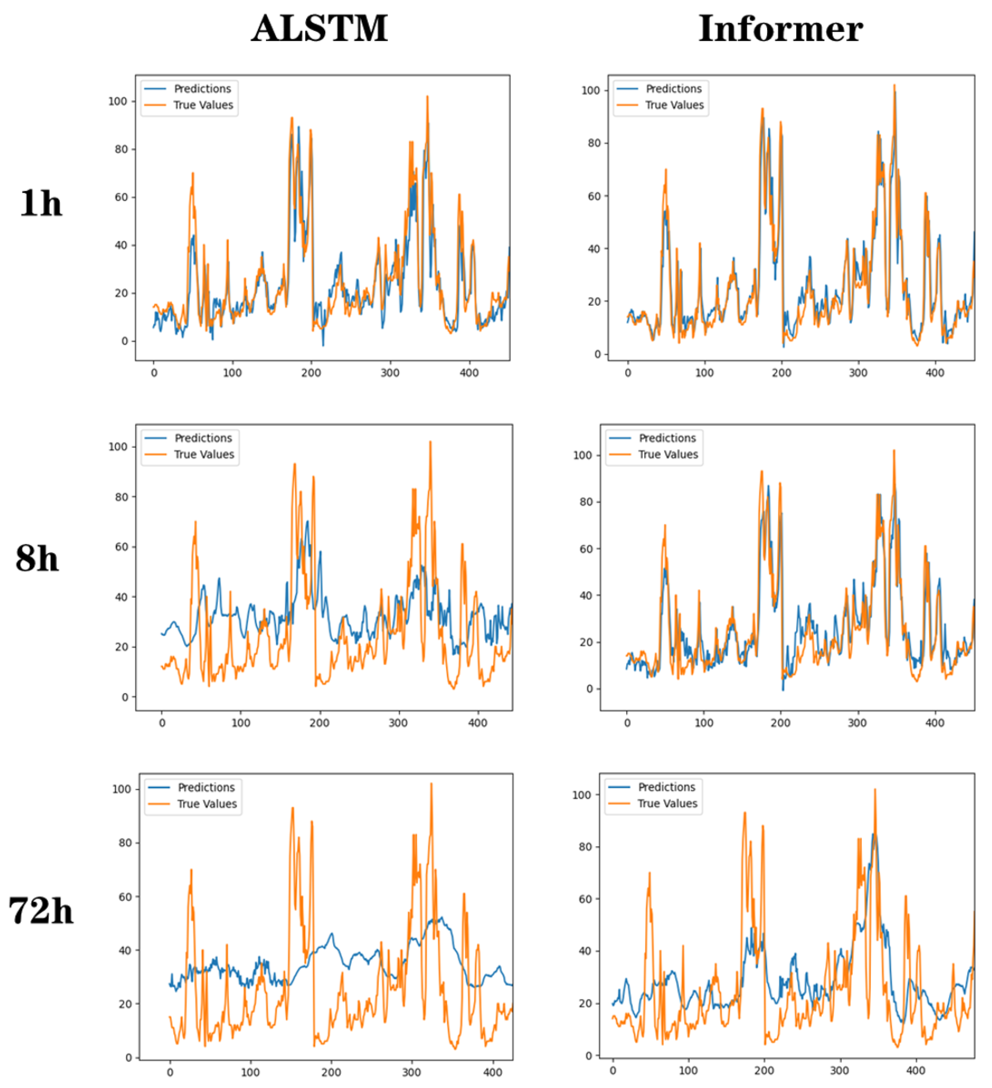
In order to validate the performance of the Informer model, this study selected LSTM and its two improved modeling methods to compare with Informer, including LSTM, CNN-LSTM, Attention-LSTM (A-LSTM), and Informer model. As with Informer, the data from January 2018 to December 2020 were used for training, the data from January to October 2021 were used for testing, and the four methods were used to predict the future PM2.5 concentrations at site 1081 A for 1 h, 8 h, and 72 h, respectively. The results are shown in Table 3, which shows that the Informer model achieves lower index results in both short and long series compared to the other methods. Figure 8 shows a visual comparison of the prediction performance of the A-LSTM and Informer. Due to the accumulation of errors, the A-LSTM model is already far from the true value when the prediction reaches the 72nd hour, while Informer still has relatively good accuracy, indicating that the Informer model has a clear advantage in long series prediction. In addition, comparing the prediction results of the models interpolated using the IDW interpolation method; it can be seen that the use of the EIDW method can lead to different degrees of improvement in the performance of the models, illustrating the effectiveness of the EIDW method.
This study compares the Informer model with a variety of improved LSTM-based methods [19,20,21,22] to demonstrate the performance advantages of the Informer model in air quality prediction, especially its significant advantage in long sequence prediction, which may be related to its decode’s model architecture of being able to output multiple tokens at once, and such a design may be helpful in reducing the accumulation of errors.

4. Conclusions

Most of the existing deep learning-based air pollutant prediction models use daily data for prediction but do not address how to deal with the missing data problem prevalent in hourly data, and applying them to hour-by-hour prediction suffers from the drawback that the prediction effect decreases rapidly as the prediction period becomes longer. Aiming at the above problems, this paper proposes an inverse distance interpolation and Informer model based on improved environmental similarity for hour-by-hour prediction of air pollutant concentrations in Taiyuan for the next 1 h, 8 h, and 72 h periods. Firstly, a multidimensional environmental vector is created for the historical air pollutant concentration data and meteorological data from seven environmental monitoring stations in Taiyuan City, from which the environmental similarity between sample points is calculated, and then the missing data in the dataset are interpolated according to the combined weight of the environmental similarity and relative distance of each sample point. After the dataset is interpolated, hour-by-hour time series prediction is performed using LSTM, CNN-LSTM, A-LSTM, and Informer, and the model performance is evaluated by statistical metrics RMSE and MAE. The experimental results show that the EIDW-Informer method is more advantageous in the hourly time series prediction of air pollutants, with an improvement of 20%, 27%, and 43% in the time scales of 1 h, 8 h, and 72 h, respectively.
However, there are some unresolved issues with this study, such as not using features that may be associated with industrial and transportation emissions to construct the environmental vectors; the Informer model discarded some minor features during training to increase the speed of training the model; and the data used came from historical observations, so it was not possible to predict anomalous events that had never occurred before. Future researchers who can find features more relevant to air pollutant concentrations or improve the coding and decoding module of the Informer model will, I believe, improve the accuracy of the hour-by-hour prediction even more.

Author Contributions

Conceptualization, K.L.; Methodology, K.L.; Software, K.L.; Validation, M.N.; Resources, H.X.; Data curation, K.L.; Writing—original draft, K.L. and H.X.; Writing—review and editing, K.L., J.S. and Y.H. All authors have read and agreed to the published version of the manuscript.

Funding

This research received no external funding.

Institutional Review Board Statement

Not applicable.

Informed Consent Statement

Not applicable.

Data Availability Statement

Data sharing is not applicable to this article.

Conflicts of Interest

The authors declare no conflict of interest.

References

  1. World Health Organization. Ambient (Outdoor) Air Quality and Health [EB/OL]. Available online: http://www.who.int/mediacentre/factsheets/fs313/en/ (accessed on 31 October 2018).
  2. Rigan, P.J.; Fuller, R.; Acosta, N.J.R.; Adeyi, O.; Arnold, R.; Basu, N.N.; Baldé, A.B.; Bertollini, R.; Bose-O’Reilly, S.; Boufford, J.I.; et al. The Lancet Commission on pollution and health. Lancet 2017, 391, 462–512. [Google Scholar]
  3. Fu, B.; Kurisu, K.; Hanaki, K. Influential Factors of Public Intention to Improve the Air Quality in China. J. Cleaner Prod. 2019, 209, 595–607. [Google Scholar] [CrossRef]
  4. Chen, Y.; Ebenstein, A.; Greenstone, M.; Li, H. Evidence on the Impact of Sustained Exposure to Air Pollution on Life Expectancy from China’ s Huai River Policy. Proc. Natl. Acad. Sci. USA 2013, 110, 12936. [Google Scholar] [CrossRef] [PubMed]
  5. Burki, T. WHO Introduces Ambitious New Air Quality Guidelines. Lancet 2021, 398, 1117. [Google Scholar] [CrossRef]
  6. Fuzzi, S.; Baltensperger, U.; Carslaw, K.; Decesari, S.; Gon, H.D.v.; Facchini, M.C.; Fowler, D.; Koren, I.; Langford, B.; Lohmann, U.; et al. Particulate matter, air quality and climate: Lessons learned and future needs. Atmos. Chem. Phys. 2015, 15, 8217–8299. [Google Scholar] [CrossRef] [Green Version]
  7. Castell, N.; Dauge, F.R.; Schneider, P.; Vogt, M.; Lerner, U.; Fishbain, B.; Broday, D.; Bartonova, A. Can commercial low-cost sensor platforms contribute to air quality monitoring and exposure estimates? Atmos. Environ. 2017, 99, 293–302. [Google Scholar] [CrossRef]
  8. Lin, C.; Labzovskii, L.D.; Mak, H.W.L.; Fung, J.C.H.; Lau, A.K.H.; Kenea, S.T.; Bilal, M.; Hey, J.D.V.; Lu, X.; Ma, J. Observation of PM2.5 using a combination of satellite remote sensing and low-cost sensor network in Siberian urban areas with limited reference monitoring. Environ. Int. 2020, 227, 117410. [Google Scholar] [CrossRef]
  9. van Donkelaar, A.; Martin, R.V. Global Estimates of Fine Particulate Matter using a Combined Geophysical-Statistical Method with Information from Satellites, Models, and Monitors. Environ. Sci. Technol. 2016, 50, 3762–3772. [Google Scholar] [CrossRef]
  10. Motlagh, N.H.; Lagerspetz, E.; Nurmi, P.; Li, X.; Varjonen, S.; Mineraud, J.; Siekkinen, M.; Rebeiro-Hargrave, A.; Hussein, T.; Petaja, T.; et al. Toward Massive Scale Air Quality Monitoring. IEEE Commun. Mag. 2020, 58, 54–59. [Google Scholar]
  11. Box, G.E.P.; Jenkins, G.M.; Reinsel, G.C.; Ljung, M.G. Time Series Analysis: Forecasting and Control; John Wiley & Sons: Hoboken, NJ, USA, 2015; pp. 47–88. [Google Scholar]
  12. Pandey, G.; Zhang, B.; Jian, L. An application of arima model to predict submicron particle concentrations from meteorological factors at a busy An application of arima model to predict submicron particle concentrations from meteorological factors at a busy roadside in hangzhou, China. Sci. Total Environ. 2012, 426, 336–345. [Google Scholar]
  13. Williams, B.M.; Hoel, L.A. Modeling and forecasting vehicular traffic flow as a seasonal arima process:Theoretical basis and empirical results. J. Transp. Eng. 2003, 129, 664–672. [Google Scholar] [CrossRef] [Green Version]
  14. Voynikova, D.S.; Gocheva-Ilieva, S.G.; Ivanov, A.V.; Iliev, I.P. Studying the effect of meteorological factors on the SO2 and PM10 pollution levels with refined versions of the sarima model. In Proceedings of the Aip Conference, AIP Publishing LLC, Albena, Bulgaria, 28 June–3 July 2015; Volume 112. [Google Scholar]
  15. Jianwei, W.; Xiaohui, C.; Feng, X.; Weiliang, L.; Jin, M. Comparative study of two different prediction models for winter aod. In Proceedings of the 2017 Eighth International Conference on Intelligent Control and Information Processing(ICICIP), Marrakesh, Morocco, 11–16 December 2017; pp. 39–43. [Google Scholar]
  16. Dai, L.J.; Zhang, C.J.; Ma, L.E.M. A dynamic model for short-term PM2.5 concentration forecasting based on machine learning. Comput. Appl. 2017, 37, 3057–3063. [Google Scholar]
  17. Bengio, Y.; Simard, P.; Frasconi, P. Learning long-term dependencies with gradient descent is difficult. IEEE Trans. Neural Netw. 1994, 5, 157–166. [Google Scholar] [CrossRef] [PubMed]
  18. Hochreiter, S.; Schmidhuber, J. Long short term memory. Neural Comput. 1997, 9, 1735–1780. [Google Scholar] [CrossRef] [PubMed]
  19. Li, X.; Peng, L.; Yao, X. Long short-term memory neural network for air pollutant concentration predictions: Method development and evaluation. Environ. Pollut. 2017, 997–1004. [Google Scholar] [CrossRef] [PubMed]
  20. Wen, C.; Liu, S.; Yao, X.; Peng, L.; Li, X.; Hu, Y.; Chi, T. A novel spatiotemporal convolutional long short-term neural network for air pollution prediction. Sci. Total Environ. 2019, 654, 1091–1099. [Google Scholar] [CrossRef]
  21. Ma, J.; Li, Z.; Cheng, J. Air quality prediction at new stations using spatially transferred bidirectional long short-term memory network. Sci. Total Environ. 2020, 705, 135771. [Google Scholar] [CrossRef]
  22. Liu, D.; Lee, S.Y. Air pollution forecasting based on attention-based LSTM neural network and ensemble learning. Expert Syst. 2019, 37, 1–16. [Google Scholar] [CrossRef]
  23. Vaswani, A.; Shazeer, N.; Parmar, N.; Uszkoreit, J.; Jones, L.; Gomez, A.N.; Kaiser, L.; Polosukhin, I. Attention Is All You Need. In Proceedings of the 31st International Conference on Neural Information Processing Systems, Long Beatch, CA, USA, 4–9 December 2017; pp. 6000–6010. [Google Scholar]
  24. Zhou, H.; Zhang, S.; Peng, J.; Zhang, S.; Li, J.; Xiong, H.; Zhang, W. Informer: Beyond Efficient Transformer for Long Sequence Time-Series Forecasting. Proc. Aaai Conf. Artif. Intell. 2021, 35, 11106–11115. [Google Scholar] [CrossRef]
  25. Shepard, D. A Two-Dimensional Interpolation Function for Computer Mapping of Irregularly Spaced data. Geography and the Properties of Surfaces. In Proceedings of the ACM National Conference, New York, NY, USA, 27–29 August 1968. [Google Scholar]
  26. Li, H.T.; Shao, Z.D. A review of spatial interpolation analysis algorithms. Comput. Syst. Appl. 2019, 28, 1–8. [Google Scholar]
  27. Lu, G.Y.; Wong, D.W. An adaptive inverse-distance weighting spatial interpolation technique. Comput. Geosci. 2008, 34, 1044–1055. [Google Scholar] [CrossRef]
  28. A-Xing, Z.; J, L.; Fei, D.; J, Z.S.; Cheng-Zhi, Q.; Jim, B.; Thorsten, B.; Thomas, S. Predictive soil mapping with limited sample data. Eur. J. Soil Sci. 2015, 66, 535–547. [Google Scholar]
  29. Lotrecchiano, N.; Sofia, D.; Giuliano, A.; Barletta, D.; Poletto, M. Spatial interpolation techniques for innovative air quality monitoring systems. Chem. Eng. Trans. 2021, 86, 391–396. [Google Scholar] [CrossRef]
  30. Buccolieri, R.; S.; berg, M.; Sabatino, S.D. City breathability and its link to pollutant concentration distribution within urban-like geometries. Atmos. Environ. 2010, 44, 1894–1903. [Google Scholar] [CrossRef]
  31. Zheng, Y.; Liu, F.; Hsieh, H.P. Uair:When urban air quality inference meets big data. In Proceedings of the 19th ACM SIGKDD international conference on Knowledge discovery and data mining, Chicago, IL, USA, 11–14 August 2013; pp. 1436–1444. [Google Scholar]
  32. Nan, S.; Liang, M.; Shi, J. Analysis of the impact of heavy pollution in Taiyuan City based on Hysplit backward trajectory model. Shanxi Sci. Technol. 2018, 33, 3. [Google Scholar]
  33. Wei-Wu, W.; Chao, C. A quantitative analysis on spatial distribution of the pollutants in the urban air and their impact factors based on geostatistics and GIS: A case study of Hangzhou city. Geogr. Res. 2008, 27, 241–249. [Google Scholar]
  34. He, K.; Zhang, X.; Ren, S.; Sun, J. Deep Residual Learning for Image Recognition. In Proceedings of the 2016 IEEE Conference on Computer Vision and Pattern Recognition (CVPR), Las Vegas, NV, USA, 27–30 June 2016. [Google Scholar]
  35. Fine, T.; Jordan, M.; Lawless, J. Feedforward Neural Network Methodology, 3rd ed.; Springer: Berlin/Heidelberg, Germany, 1999; pp. 18–156. [Google Scholar]
  36. Li, S.; Jin, X.; Xuan, Y.; Zhou, X.; Chen, W.; Wang, Y.; Yan, X. Enhancing the locality and breaking the memory bottleneck of transformer on time series forecasting. In Proceedings of the NIPS’19: Proceedings of the 33rd International Conference on Neural Information Processing Systems, Vancouver, BC, Canada, 8–14 December 2019. [Google Scholar]
  37. Zhou, T.; Ma, Z.; Wen, Q.; Wang, X.; Sun, L.; Jin, R. FEDformer: Frequency Enhanced Decomposed Transformer for Long-term Series Forecasting. In Proceedings of the International Conference on Machine Learning, Baltimore, MD, USA, 25–27 July 2022; pp. 27268–27286. [Google Scholar]
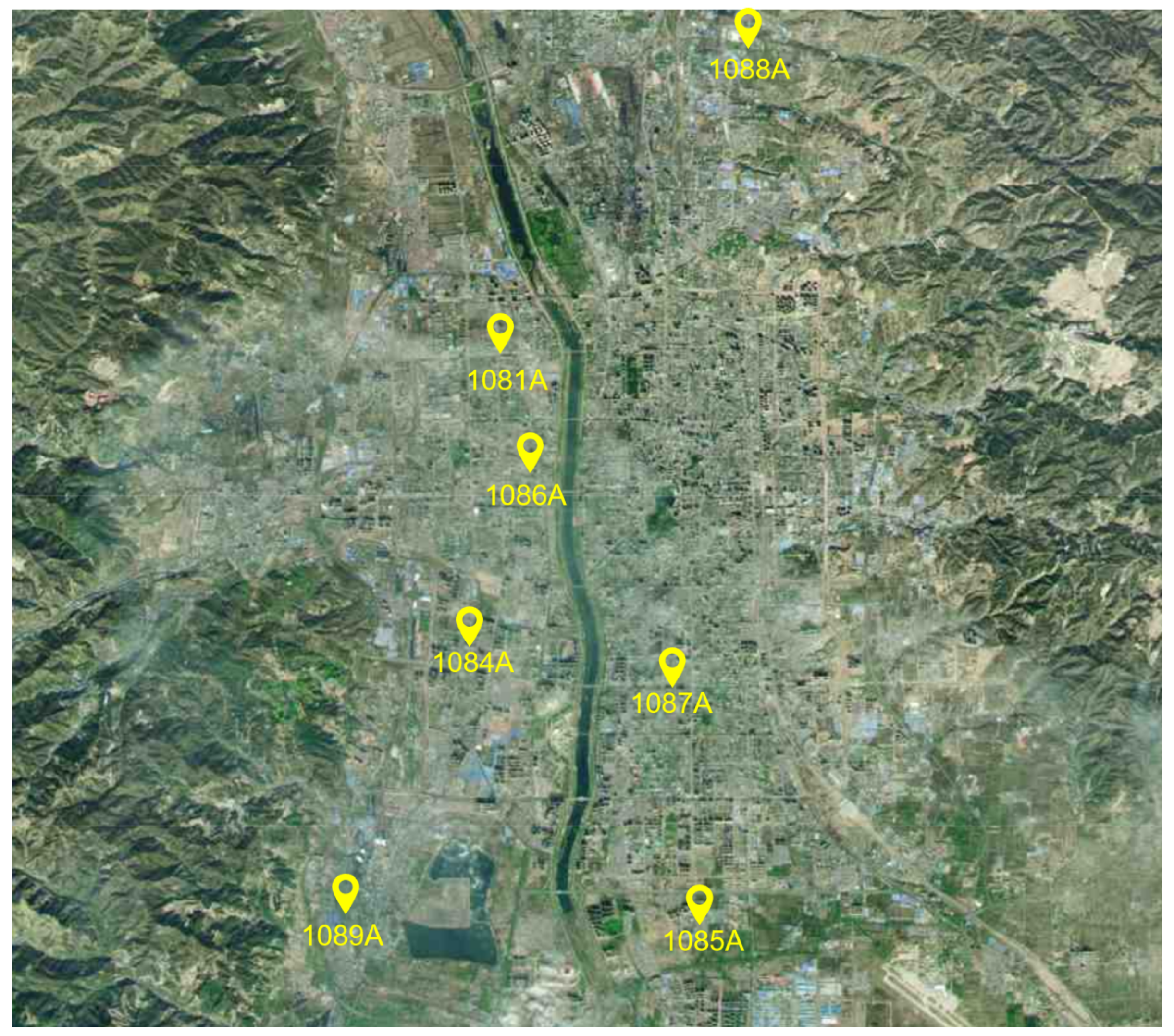
Figure 1. High-resolution map of Taiyuan city, yellow signs indicate the location of air monitoring stations.
Atmosphere 14 01274 g001
Figure 2. P i is the point to be predicted and P 1 , P 2 , P 3 , P 4 , P 5 are the sample points.
Atmosphere 14 01274 g002
Figure 3. The correlation test result for PM2.5.
Atmosphere 14 01274 g003
Figure 4. The correlation test result for NO2.
Atmosphere 14 01274 g004
Figure 5. The correlation test result for O3.
Atmosphere 14 01274 g005
Figure 6. The model structure of the Transformer. X d e is decoder input, X 0 consists of random values, *6 indicates six layers of the same structure.
Atmosphere 14 01274 g006
Figure 7. The model structure of Informer. X d e is the decoder input, X t o k e n is the start token that the true values of the predicted features in the most recent hours, X 0 also consists of random values, representing the token to be predicted, *6 indicates six layers of the same structure.
Atmosphere 14 01274 g007
Figure 8. Model prediction performance comparison chart. The vertical coordinate of the graph is the real-time concentration of PM2.5 in micrograms per cubic meter, and the horizontal coordinate is the time in hours.
Atmosphere 14 01274 g008
Table 1. Performance comparison of the EIDW and IDW methods.
Interpolation MethodEvaluation IndicatorsPM2.5NO2O3
EIDWRMSE16.3218.0126.14
MAE12.9016.9524.23
IDWRMSE18.3022.4327.93
MAE15.7220.3825.11
Table 2. Prediction of PM2.5, NO2 and O3 pollutant concentrations by the Informer model.
PollutantEvaluation Indicators1 h8 h72 h
PM2.5RMSE7.2116.4419.33
MAE4.8612.5616.65
NO2RMSE9.9218.9721.09
MAE6.8914.1915.58
O3RMSE11.4621.1030.28
MAE7.7618.8122.72
Table 3. Informer, LSTM, CNN-LSTM, ALSTM, ALSTM (interpolated using the IDW method), Informer (interpolated using the IDW method) for PM2.5 concentration prediction.
ModelsEvaluation Indicators1 h8 h72 h
InformerRMSE7.2116.4424.67
MAE4.8612.5621.05
LSTMRMSE10.9225.6948.06
MAE8.9718.8732.43
CNN-LSTMRMSE8.7522.3546.11
MAE5.8915.1229.51
ALSTMRMSE8.3420.5441.64
MAE6.1014.8226.10
ALSTM (IDW)RMSE9.0322.6143.04
MAE6.7616.1727.87
Informer (IDW)RMSE7.9518.0928.02
MAE5.9413.2424.85
Disclaimer/Publisher’s Note: The statements, opinions and data contained in all publications are solely those of the individual author(s) and contributor(s) and not of MDPI and/or the editor(s). MDPI and/or the editor(s) disclaim responsibility for any injury to people or property resulting from any ideas, methods, instructions or products referred to in the content.