Article

Machine-Learning-Based Lithosphere-Atmosphere-Ionosphere Coupling Associated with Mw > 6 Earthquakes in America

by
Munawar Shah
1,*,
Rasim Shahzad
1,
Punyawi Jamjareegulgarn
2,
Bushra Ghaffar
3,
José Francisco de Oliveira-Júnior
4,
Ahmed M. Hassan
5 and
Nivin A. Ghamry
6
1
Department of Space Science, GNSS and Space Education Laboratory, National Center of GIS & Space Applications, Institute of Space Technology, Islamabad 44000, Pakistan
2
Department of Electrical Engineering, Faculty of Engineering, King Mongkut’s Institute of Technology Ladkrabang, Prince of Chumphon Campus, Chumphon 86160, Thailand
3
Department of Environmental Science, Faculty of Sciences, International Islamic University, Islamabad 44000, Pakistan
4
Laboratório de Meteorologia Aplicada e Meio Ambiente (LAMMA), Instituto de Ciências Atmosféricas (ICAT), Universidade Federal do Alagoas (UFAL), Maceio 57072-260, Brazil
5
Faculty of Engineering, Future University in Egypt, Cairo 11835, Egypt
6
Faculty of Computers and Artificial Intelligence, Cairo University, Giza 12613, Egypt
*
Author to whom correspondence should be addressed.
Atmosphere 2023, 14(8), 1236; https://doi.org/10.3390/atmos14081236
Submission received: 5 July 2023 / Revised: 27 July 2023 / Accepted: 28 July 2023 / Published: 31 July 2023
(This article belongs to the Special Issue State-of-the-Art in Gravity Waves and Atmospheric-Ionospheric Physics)

Abstract

:
The identification of atmospheric and ionospheric variations through multiple remote sensing and global navigation satellite systems (GNSSs) has contributed substantially to the development of the lithosphere-atmosphere-ionosphere coupling (LAIC) phenomenon over earthquake (EQ) epicenters. This study presents an approach for investigating the Petrolia EQ (Mw 6.2; dated 20 December 2021) and the Monte Cristo Range EQ (Mw 6.5; dated 15 May 2020) through several parameters to observe the precursory signals of various natures. These parameters include Land Surface Temperature (LST), Air Temperature (AT), Relative Humidity (RH), Air Pressure (AP), Outgoing Longwave Radiations (OLRs), and vertical Total Electron Content (TEC), and these are used to contribute to the development of LAIC in the temporal window of 30 days before and 15 days after the main shock. We observed a sharp increase in the LST in both the daytime and nighttime of the Petrolia EQ, but only an enhancement in the daytime LST for the Monte Cristo Range EQ within 3–7 days before the main shock. Similarly, a negative peak was observed in RH along with an increment in the OLR 5–7 days prior to both impending EQs. Furthermore, the Monte Cristo Range EQ also exhibited synchronized ionospheric variation with other atmospheric parameters, but no such co-located and synchronized anomalies were observed for the Petrolia EQ. We also applied machine learning (ML) methods to confirm these abrupt variations as anomalies to further aid certain efforts in the development of the LAIC in order to forecast EQs in the future. The ML methods also make prominent the variation in the different data.

1. Introduction

Earthquakes (EQ) cause immense devastation and are responsible for multiple casualties every year through enormous destruction at the local as well as the regional scale (depending upon the magnitude) [1,2,3]. They occur due to the tectonic stress variations at various depths of the Earth’s lithosphere, leading to intense shaking and brittle failures that are linked to the main shock [4]. EQs play a significant role in aggregating and releasing energy to the atmosphere and ionosphere. However, scientists have often suggested that the complex nature of EQs makes predicting them a difficult challenge [4]. In spite of years of research, several geological parameters and physical phenomena used as precursors are still under debate. Geller [5] portrayed EQ forecasting in a pessimistic manner; however, Keilis-Brook [6] suggested that future technology would play a key role in EQ forecasting as a holistic approach is needed to predict a complex system of mechanisms. Satellite-based observations are evolving into effective tools for this objective, showing momentary anomalies that precede EQs [3,7,8,9]. Recently, various space instruments recorded significant variations in the surface temperature, deformations in the Earth’s surface, aerosols that exhaled atmospheric gases, and electric field disturbances in the ionosphere [10,11,12]. These disturbances can be observed generally within 20 days before and/or 10 days after the main shock in the atmosphere, and this is followed by a significant variation within 5 days before and after in the ionosphere, which serve as EQ precursors. In the main, possible atmosphere and ionosphere anomalies can be observed in three regions from the satellite observations over the epicenter of the Earth’s surface [12,13,14,15,16,17,18]. However, statistical analyses have showed that positive anomalies are more prominent than negative ones that have shallow hypocentral depth and large magnitude [19]. Shah et al. [20] suggested that, in order to observe clear perturbations over the epicenter, the hypocentral depth should be less than 20 km with a magnitude greater than 6. More studies have shown that seismic anomalies are possible, but Masci and Thomas [21] claimed that the existing satellite cluster makes ionospheric anomalies impossible. Moreover, Pulinets et al. [22] and Su et al. [23] also emphasized that storm time ionospheric anomalies are more pronounced than seismic activity; moreover, they suggested that it is possible to observe EQ anomalies during quiet storm conditions. They further suggested that more explanation is required about how these anomalies are linked with seismic main shocks.
During the anomaly generation process related to EQs, several changes occur as precursors at the Earth–atmosphere interface as a result of anomalous electric fields within the epicentral regions. Many researchers have explained EQ anomalies prior to a main shock during the seismic preparation period [3,8,20,24,25]. Moreover, the atmosphere and ionosphere anomalies can be discussed on the basis of different mechanisms in the LAIC hypothesis. For example, Pulinets and Ouzounov [8] suggested that, prior to substantial EQs, radon gas is released into the atmosphere along with other gases (serving as carriers) like carbon dioxide, helium, methane, and hydrogen. Where atmospheric anomalies are created due to air ionization, which are caused by radon and with water vapor condensation, the latent heat of vaporization is created. Furthermore, ion cluster production at the atmospheric boundary layer under the effect of variations in the atmospheric electric field causes a local alteration in the global electric circuit, which causes abnormalities in the ionosphere [8]. Moreover, they reported that a chain of reactions in the atmosphere after the emanation of radon, along with greenhouse gases, upon reaching the surface can enhance surface temperature, a decrement in humidity due to the cooling of gases and radon, aerosol particle formation, changes in the atmospheric electric conductivity, and electric couplings creating ionospheric variations. There are also ionospheric anomalies that occur due to electric field disturbances [26] and high-energy particle flux [27] over the epicentral region. However, Freund [28] proposed the theory of positive hole (p-hole) generation from the stressed-rock conditions that rise up in the atmosphere, producing anomalous behavior in the ionosphere that lead to delays in radio signal propagation. These p-holes move from stressed-rock to unstressed-volume conditions, which is followed by its traveling to the Earth’s surface to interact with the air particles and building air ionization processes over the EQ preparation zone. A battery-like situation is created if the crust of the Earth is taken as one side of a battery; moreover, electromagnetic radiations and pulses toward the atmosphere are produced under the action of stress along fault lines [28]. Ultimately, the anomalies are created over the impending EQ epicenter under the influence of the aforementioned processes, destabilizing the ionosphere’s lower part [3,29,30]. Both of the above theories explain the LAIC hypothesis that is associated with main shocks.
Prior to EQs, multiple studies using different methods have been published. For example, Ouzounov et al. [31] studied the anomalous behavior in the atmosphere as well as the ionospheric parameters within 5 days prior to the main shock of the Tohoku-Oki (M 9.1) earthquake. Additionally, Shi et al. [32] found positive as well as negative anomalies in the ionosphere when using ground-based receivers for the Nepal EQ Mw 7.8. However, a clear definition of atmospheric and ionospheric anomalies as EQ precursors has yet not been established. The ionospheric anomalies associated with the 1279 EQs of Mw > 6 during 2000–2014 showed no clear relation with the foreshocks due to fewer satellite clusters [33]. Furthermore, an anomalous rise in LST was observed within the 7-day window prior and 2 days after the main shock of the 2013 Awaran EQ [13]. Moreover, Ouzounov et al. [31] reported pre-EQ anomalies in the time window during 4–14 days. Significant OLR anomalies also occurred in the atmosphere associated with the Jamaica EQ event with a clear rise of more than 30 W/m2 [34]. Furthermore, AT and AH variations due to LAIC were also reported in previous reports [35,36]. Although, many studies have been performed on this topic, there is a huge gap in the knowledge in EQ prediction.
In this paper, we analyze the atmospheric and ionospheric anomalies for two EQs occurred in the North American region for the possible anomalous patterns. To further verify the LAIC hypothesis, these two events were considered during quiet storm conditions to show the association of anomalous parameters for unusual behavior in atmosphere and ionosphere as EQ precursors. We analyzed the behavior of various layers, i.e., lithosphere, atmosphere and ionosphere, to observe a synchronized pattern of anomalies over both the epicenters. To better understand the impact of an EQ on these three layers, we analyzed the data with various methods like statistical, wavelet and machine learning approaches. In contrast to the past studies, this paper studies the EQ precursors using data from multiple satellites by utilizing different techniques. In this paper, we studied the Materials and Methods in Section 2. Furthermore, the Results and Discussion are included in Section 3 and Section 4, respectively. Finally, Section 5 provides the Conclusion.

2. Materials and Methods

2.1. Study Area

In this paper, we analyzed the temporal variations of multiple atmospheric layers over the epicenters of two EQs in the North American region. One of the EQs struck the region during the winter season at Lat = 40.3°and Lon = −124.2°, having a shallow depth of 27.1 km and Mw 6.2. According to the preliminary analysis, the Mw 6.2 event occurred within 7 km onshore from the North of Petrolia, and is generally regarded as the EQ in the Gorda plate. While, the other EQ occurred in summer with epicenter was in the Monte Cristo Range. The latitude and longitude of the Monte Cristo EQ was 38.1° and −117.85°, respectively. It occurred at a shallow depth of 2.7 km beneath the Earth. This EQ was followed by multiple aftershocks within 5 hours of the main shock at a magnitude 4.5 and higher. As both of these EQs were Mw > 6, these caused abrupt shaking around the epicenters and the affected areas are showed in Figure 1. More information about these two events can be found on the website of the United States Geological Survey (USGS) (https://earthquake.usgs.gov/earthquakes/map/; accessed on 20 January 2023).

2.2. Datasets

2.2.1. Land Surface Temperature (LST)

The thermal infrared anomalies were very notable during the preparation period of the EQs over the epicenters [4,36]. For this, we considered the LST retrieved from the MODIS on board the Terra satellite on 18 December 1999. The data are available for the whole globe on diurnal basis, having a swath width of 2330 km in 36 spectral bands (http://modis.gsfc.nasa.gov/data; accessed on 20 January 2023). For both the EQs in this paper, 46 days of data were obtained in the form of 30 days before and 15 days after the main shock day to find anomalous time window. Furthermore, an average of the previous five years of LST for the same region during the same days was used to compare the trend and find out an anomaly from the normal distribution around the epicenters.

2.2.2. Outgoing Longwave Radiation (OLR)

The combination of emission from the ground, lower atmosphere and clouds is named as OLR and it has been used to investigate the anomalous distribution in atmosphere by the EQ energy. Furthermore, it is one of the most vital parameters for assessing the radiation emitting from Earth during the EQ preparation period [3,37]. The Goddard Earth Science Data and Information Service Center (GES DISC) were utilized to access the OLR data from AIRS/Aqua at a 1-degree spatial resolution. Furthermore, an area averaged OLR time series are analyzed over epicenters for both the EQs (https://disc.gsfc.nasa.gov/; accessed on 20 January 2023).

2.2.3. Relative Humidity (RH)

The RH is a ratio between the saturated vapor pressure and measured water vapors at a specific temperature and it can be used to find the anomalous responses at troposphere–stratosphere exchange over the EQ epicenters. For both the EQs, RH data were retrieved from the NOAA Physical Science Laboratory NCEP-NCAR (http://psl.noaa.gov/data/composites/day/; accessed on 20 January 2023). The interval of these data was a 46-day window (30 days before and 15 days after the main shock day) around the main shocks.

2.2.4. Air Temperature (AT)

We acquired the AT data from the National Oceanic and Atmospheric Administration (NOAA) with a spatial resolution of 2.5° (Latitude) × 2.5° (Longitude) for the same period of 46 days (30 days before and 15 days after the main shock day) to observe a correlation between the seismic activity and atmospheric anomalies. These data were accessed from the NCEP/NCAR reanalysis project (http://psl.noaa.gov/data/composites/day/; accessed on 20 January 2023).

2.2.5. Air Pressure (AP)

In this paper, we also analyzed the AP data over the epicenters for 30 days before and 15 days after the main shocks. The AP is a force exerted by the air under the action of gravity over surface of the Earth. We acquired these data from the NOAA reanalysis project, named the NCEP/NCAR, over the EQ epicenters from different satellites.

2.2.6. Total Electron Content (TEC)

We analyzed the behavior of ionosphere in response to both EQs by retrieving TEC from multiple GNSS stations around the epicenters. To assess the Seismo Ionospheric Anomalies (SIAs), various GNSS stations were selected in such a manner that some stations were operating within the vicinity of the EQ preparation zone; while, some were operating outside the EQs impacted area (Table 1). Moreover, the geomagnetic indices were also considered to observe the storm activity and further differentiate the geomagnetic-storm-induced anomalies from SIAs of the main shocks. These indices were retrieved from the Space Physics Data Facility of the Goddard Space Flight Center (http://omniweb.gsfc.nasa.gov/; accessed on 20 January 2023).
The TEC for all the selected GNSS stations operating within or outside the vicinity of the EQ preparation zone were retrieved using the tool provided at: www.ionolab.org (accessed on 20 January 2023). To examine the behavior of the ionosphere in response to an EQ, Vertical TEC was calculated using the below equations in the TEC Unit (where 1 TECU = 1016 el/m2). Furthermore, the slant TEC was used to calculate VTEC using the below equations [38].
T E C a h = ( f 1 2 f 2 2 ) 40.3 ( f 1 2 f 2 2 ) ( P 4 , a h c . D C B a c . D C B h )
V T E C = S T E C × cos [ arcsin R s i n z R + H ]
where ( f 1 2 , f 2 2 ) are dual frequencies at receiver from the GPS stations, P 4 , a h is the difference between the smoothed coded measurements, c is the speed of light and D C B h and D C B a are the differential code biases for GPS and satellite receiver, respectively. Similarly, R is the Earth’s radius, z is the zenith angle of the satellite and H is the ionospheric height (in this paper, we considered 350 km).

2.3. Methods

In this paper, we studied multiple atmospheric and ionosphere possible precursory signals within the EQs preparation zones over the epicenters in the Dobrovolsky region. The EQ preparation zone can be calculated using the Dobrovolsky et al. [39] equation.
R D = 10 0.43 × M
In the above equation, the EQ impacted zone is shown as RD in kilometers and M represents the magnitude of the EQ. Using the formula, the epicentral zones for the Petrolia and the Monte Cristo Range EQs were estimated to be 463 and 627 KMs around the epicenters, respectively. Previous researchers mentioned that the anomalies in LAIC coupling became more prominent inside the Dobrovolsky region in comparison to outside the epicentral zone [18,31,40,41].

2.3.1. Anomaly Detection Using Interquartile Ranges Method

The bounds of all the time series were analyzed under the Interquartile Ranges (IQRs), in which any value crossing above or below the specified bound from the normal distribution were considered as anomalies. IQR is a statistical approach for dividing the datasets into four quartiles to quantify the variations in a statistical dispersion. In an IQR method, the data are divided into four quartiles to show the maximum variations associated with the EQs. Most of the previous reports used the median and IQR method to confirm the anomalous behavior of atmospheric parameters due to a non-linear data distribution in comparison to a Gaussian probability function [3,37,42]. The below equations can be used to calculate the bounds for this paper.
xhigh = M + k × IQR
xlow = Mk × IQR
xlow < x < xhigh k < x M I Q R < k
D x = x M I Q R
In the above equations, the original atmospheric parameters are represented as x, upper bound as xhigh, lower bound as xlow and median of dataset as M. Similarly, IQR and Dx are the interquartile range and differential of x, respectively.
The anomalous behavior of the analyzed atmospherics parameters was subjected to a condition with an absolute value of Dx greater than k (i.e., |Dx| > k). Moreover, the anomalous pattern in any parameter was declared to be with 66% of confidence level with the observed atmospheric parameter, either crossing the upper bound or dropping below the lower bound [3,37,43]. Using the above procedures, the confidence bounds of all the parameters were calculated using the median and IQRs of all the data from 30 days before and 15 days after the main shock.

2.3.2. Anomaly Detection Using Neural Network

Neural Network (NN) is an intelligence-based system that can model any atmospheric phenomenon based on the relationship, recognized pattern and some prior assumptions. Neurons are connected in a NN method by the number of weighted connections that store the information. The weights of the network’s connections are mainly determined by the training process. The prediction errors exceeding any predetermined threshold indicate abnormal variations or anomalies in the measured values.
In this study, multiple LAIC anomalies were confirmed using a nonlinear autoregressive with exogenous inputs (NARX) network for both the EQs. In the artificial neural network, NARX represented a nonlinear dynamic time series system [14,44]. Using the NARX network architecture for a time series, the independent input signal and output signal were regressed against the dependent output signal y (t) estimation. To find anomalies in this paper, 70% of data were used for training with 15% for the validation and 15% for testing purposes. The flow chart of NARX can be seen in Figure 2.
The equation for the NARX model is given below.
y   ( t )   =   f   ( y   ( t 1 ) ,   y   ( t 2 ) ,   ,   ( t n y ) ,   x   ( t 1 ) ,   x   ( t 2 ) ,   ,   x   ( t n x ) )
The output lags, input lags, hidden layers, neurons and activation functions were acquired iteratively in order to establish the efficient training of a network architecture with minimal estimation error. The linear and sigmoid activation functions were used in both the hidden and output layers to specify the optimal outcomes. For faster convergence, the Levenberg–Marquardt algorithm includes hundreds of weights to address the function approximation problems [3,37]. To train the algorithm, the Levenberg–Marquardt method was used. Additionally, the N observations were used to produce the predictions, including y1, y2, yN and yN + 1, yN + 2,..., yN + m as test and training sets, respectively. The input layer, hidden layer and output layer consisted of six nodes, ten nodes and one node, respectively. For this analysis, the corrected values, their corresponding time, the mean value and the deviated parameters from the mean value were used as input values. We also used the time series of the lithosphere, the diurnal series of atmosphere parameters and hourly ionospheric TEC with their mean values, their corresponding time, and the deviation from the normal distribution as input layers to obtain the output layer over the epicenters within the Dobrovolsky region. The training patterns for networks are shown below.
y4 = f (y1, y2, y3, t1, t2, t3)
y5 = f (y2, y3, y4, t2, t3, t4)
yN = f (yN−3, yN−2, yN−1, tN−3, tN−2, tN−1)
By finding the optimized weights according to the equation below, we minimized the prediction error (PE).
PE = k 0 N ( y ^ ( t k ) y ( t k ) ) )
Here, the output of the network is y ^ .
The testing patterns are shown below.
yN+4 = f (yN+1, yN+2, yN+3, tN+1, tN+2, tN+3)
yN+5 = f (yN+2, yN+3, yN+4, tN+2, tN+3, tN+4)
yN+m = f (yN+m−3, yN+m−2, yN+m−1, tN+m−3, tN+m−2, tN+m−1)
Using the above equations, the anomalous value was obtained by comparing the predicted values with the actual values beyond the defined bounds [3,14].

3. Results

In this study, we analyzed various lithospheric, atmospheric and ionospheric parameters by applying statistical, wavelet and ML techniques to provide substantial LAIC evidence for the two North American EQs. The anomalies at various altitudes above the epicenters of the impending EQs were studied in the form of lithosphere, atmosphere and ionosphere variations. These different anomalies are discussed in detail below.

3.1. Petrolia EQ

To observe the LAIC hypotheses to the impending American EQs, we studied first the variations in LST, AT, AP, OLR and RH, along with TEC, from GNSS stations for the Petrolia EQ for 30 days before and 15 days after the main shock.
We analyzed both the daytime and nighttime LST trend over the epicenter as the lithosphere variations in the LAIC hypothesis related to the Petrolia EQ within the Dobrovolsky region. To emphasize the anomalous variations, we also calculated the 5 year (2016–2020) mean trend as a background for the same days from 20 November 2021 to 4 January 2022 over the same region. For this event, we observed a clear rise of 4 °C within 6 days before the main shock in the day time series, followed by a sudden drop of 5 °C after the main shock day (Figure 3a).
According to our observations, temperature was dropping towards the main shock day. The mean for both the day-and night-time LST values is also clear from the background of the past 5 years. We noticed a variation of only 1–2 °C from the background value on normal days before the main event by comparing the LST values with the past 5 year averaged time series. However, a difference of more than 4 °C was observed on the anomalous day as the sixth day before the main shock. On the contrary, the time series of the nighttime LST over the same region depicted a rise of 6 °C on the fifth day before the main shock (Figure 3b). This was also confirmed by the 5-year trend of the past LST. Additionally, a difference of more than 5 °C in the original LST and 5-year trend was recorded in the nighttime. Furthermore, NARX predicted values of both the day- and nighttime confirmed our results regarding abrupt variations (Figure 4a,b). In Figure 4a’, the difference between the predicted and observed values was between −3 and +3 on 14th December during the sixth day window before the main shock (i.e., 6 °C). Similarly, we also observed the maximum deviation between the calculated and observed time series of nighttime LST of >5 °C during the 5-day window before the main shock, as shown in Figure 4d. The difference in the values from the night- and daytime depicted a value of >2.5 °C as an anomaly with respect to the confidence bounds for both the time series (Figure 4a’,b’).
Furthermore, the atmospheric anomalies of the Petrolia EQ were also observed as clear variations in AT, RH, OLR and AP within the same time window of 30 days before and 15 days after the main event (Figure 5). We observed a clear drop in the atmospheric temperature on the sixth day before the EQ (Figure 5a). Moreover, RH showed a drop of 16–18% on 14th December on the sixth day before the main shock as a possible EQ anomaly. Furthermore, the RH dropped by 4% below the confidence bound on the same day. We also observed a sharp increase in AP on 14th December, depicting a positive anomaly of 5 mb beyond the upper bound. However, the anomalous variation was up to 17 mb beyond the defined confidence bound (Figure 5c). On the other hand, OLR showed positive variations of 10 W/m2 on December 14th before the Petrolia EQ with respect to upper bound (Figure 5d).
To confirm these anomalies, the ML algorithm in the form of NARX was implemented on various atmospheric parameters to clear the variations (Figure 6). In Figure 6a, it is clear that the NARX predicted values followed the observed AT pattern on the same day of 14th December (sixth day before the main shock), as in the statistical analysis. We observed the maximum deviation between the predicted and the observed values, which also exhibited clear variations beyond the lower bound, as in Figure 5a, depicting a sharp decrease from the normal deviation (Figure 6a’). Similarly, the RH also showed similar behavior with clear variation on the sixth day before the main shock day. We observed a sharp decrease in the observed RH value. On the contrary, NARX predicted RH showed no such abrupt variations in Figure 6b. On 14th December, a maximum deviation of 16% was noted between the observed and the predicted values. However, this anomaly was only 5% in magnitude beyond the bound, as shown more clearly in the statistical analysis (Figure 6b’). While comparing the observed AP and predicted AP, we noticed 29.7 mb and 18.8 mb on 13th December in the observed values and NARX predicted values, respectively. The difference in both the observed and predicted values was more than 10 mb. A deviation peak of 8.6 mb was also obtained in NARX method on 14th December to further confirm the anomalous value observed in the statistical analysis. On the contrary, statistical analysis also confirmed the AP anomaly on 14th December on the sixth day before the main shock. Both the anomalies of 13th and 14th December observed a deviation in AP from the NARX predicted values as positive anomalies of the values of 4 mb and 6 mb, respectively (Figure 6c’). Additionally, a large discrepancy of 59.1 W/m2 in the OLR time series between the observed and the predicted values is seen in Figure 6d. We can observe a clear positive anomaly of 19.8 W/m2 beyond the upper bound in Figure 6d’. Apart from the anomalous days, no clear deviation was observed beyond the confidence bounds for all the atmospheric parameters.
The ionosphere TEC variation of four GPS stations is shown in Figure 7 for the possible anomalies of the Petrolia EQ. These stations were operating inside and outside the Dobrovolsky region (detail in the caption of Figure 7b–e). Furthermore, the geomagnetic indices of Dst and Kp were also plotted to differentiate the EQ-induced anomalies from that of the geomagnetic storm (Figure 7a,b).
During the Petrolia event, the ionospheric anomalies occurred in a quiet storm condition before the main shock. All the four stations exhibited a similar pattern of anomalous rise in TEC values on 18th December (two days before the main shock, as Mw 6.2 occurred on 20 December 2021) of twice the maximum value of TEC of 17th December. These variations, when compared to the Dst and Kp index, depicted that these were storm-induced anomalies and not the EQ anomalies, as both of these parameters showed minor geomagnetic activity (Dst < −30 and Kp = 4) on 18th December (Figure 7a,b). Furthermore, we also applied the NARX technique to observe the maximum deviation between the observed and the predicted TEC of all the GNSS stations on the same day (i.e., 18th December) for confirmation of the anomalous variations (Figure 8). A similar pattern of anomalous variations was depicted by all the stations whether operating inside or outside the Dobrovolsky region (Figure 7b–f and Figure 8e). Many researchers believed that TEC anomalies can only occur in the values of a GNSS station operating inside the EQ preparation zone. Thus, these cannot be termed as EQ-induced anomalies. On the contrary, multiple other lithosphere and atmosphere parameters confirmed the anomalous pattern within the 6–7 days before the main shock using both statistical and ML approaches (Figure 3, Figure 4, Figure 5 and Figure 6).

3.2. Monte Cristo Range EQ

We also analyzed the LAIC phenomena for the impending EQ of the Monte Cristo Range on 15 May 2021. For this, we also used the statistical, ML and wavelet methods to study the anomalies. The time window of 46 days was also taken for this event, 30 days before and 15 days after the main shock.
The LST variations associated with the impending EQ for both the day- and nighttime showed clear lithospheric variations with the Monte Cristo Range event (Mw 6.5 occurred on 15 May 2020). Furthermore, the anomalous behavior of LST was clear by plotting the daily LST against the 5-year LST trend (from 2015 to 2019 in the same region) within the Dobrovolsky region around the epicenter of the Monte Cristo Range EQ (Figure 9). While analyzing the results, we noticed a clear increase of 13 °C on 8th May against the 5-year background LST, followed by a sudden drop of 11 °C on the next day. Although LST was increasing day by day with respect to the summer season, an abrupt peak on 8th May was exhibited in the daytime LST. A maximum deviation of 12 °C was observed between the observed LST and the 5-year LST trend on the seventh day before the impending EQ (Figure 9a). On the other hand, no such abrupt variation occurred other than a rise of 3 °C on the night of 8th May, against the background of the 5-year LST trend. But, this rise was not so much substantial when compared to the 5-year nighttime LST trend (Figure 9b).
To further confirm these anomalies, ML was applied on both the time series (Figure 10). We analyzed the anomalous behavior of the daytime LST from the direct MODIS data and the NARX predicted LST (Figure 10a,a’). The NARX underestimated the observed LST by 11.13 °C on 9th May (sixth day before the main shock). Furthermore, the anomaly became more clear by applying the confidence bounds for more than 8 °C beyond the lower bound on the sixth day before the main shock in Figure 10a’. We also observed no anomalies in our statistical analysis of the nighttime LST in Figure 8b. However, the ML approach also provided a substantial anomalous rise of 1.5 °C beyond the upper bound on 11th May (4 days before the EQ event hit the region) in Figure 10b,b’.
We also studied multiple atmospheric parameters in the form of AT, RH, AP and OLR for the Monte Cristo Range EQ in Figure 11a–d. In Figure 11a, a sharp positive peak was observed beyond the upper bound on 8 May 2020. The value of all the 46 days retrieved AT was within 280 °C–290 °C, except on the anomalous day (anomalous day was 301.2 °C). Similarly, RH depicted a sharp negative peak of 35.2% on the same day. The negative anomaly of 8.8% was also observed using the confidence bounds method below the lower bound (Figure 11b). However, AP exhibited no such anomalies before the main shock within the similar day window, but there were minor abrupt variations beyond the upper bound on the sixth day after the main shock (Figure 11c). While studying the OLR variations, we noticed a 24 W/m2 rise in OLR on 8th May beyond the upper bound, followed by a sharp decrease of 30 W/m2 after the anomalous day. The statistical analysis showed a positive anomaly of 4.7 W/m2 on the same day, confirming the abrupt variations of OLR in the same time window of other atmospheric anomalies (Figure 11d).
Furthermore, we also analyzed all these parameters using ML by employing NARX to detect the anomalous behavior of the datasets (Figure 12). We observed a significant deviation of 9.3 K between the observed AT and NARX predicted AT on the seventh day before the main shock (Figure 12a). Similarly, a positive anomaly of 5 K was depicted over the confidence bounds, confirming the results of the statistical method (Figure 12a’). A similar pattern was also observed by RH with a negative peak of 20.1% below the lower bound on the seventh day before the main shock. Furthermore, the difference between the observed and the predicted RH was maximum on the same day, depicting an anomaly of 11.9% beyond the confidence bounds (Figure 12b,b’). However, AP showed no substantial evidence of an abrupt variation due to the impending EQ like the anomaly seen using the statistical analysis method (Figure 12c,c’). In the case of the OLR variations, we noticed a 295.2 W/m2 variation on 8th May and the NARX predicted OLR had a variation of 264.4 W/m2. Other than the 8th May deviation between the observed and predicted OLR values, these were less than 10 W/m2. Furthermore, an anomaly of 12.1 W/m2 was observed by applying the confidence bounds method on 8th May (Figure 12d,d’).
The ionosphere anomalies were studied for the Monte Cristo Range EQ from the TEC variations of four GNSS stations including COSO, QUIN, DRAO and HOLD (Figure 13). The COSO and QUIN were operating within the Dobrovolsky region and the rest of the stations were operating outside of the region of the EQ preparation. For this event, we also analyzed the Dst and Kp indexes to find out the relationship of ionospheric anomalies with the geomagnetic activity near the EQ event (Figure 13a,b). In the COSO station, minor variations were exhibited in the ionosphere on 8th May, whereas a prominent increase of 5 TECu was visible on 9th May against the previous 10 day trend of the TEC in the ionosphere (Figure 13c). However, the TEC values were, again, within the normal trend during the next days as we moved towards the EQ event. Similarly, the QUIN station retrieving the TEC showed a rise of 18.1 TECu on 9th May. The anomaly was 6 TECu more than the normal TEC distribution in the specific region according to the data variations. A minor abrupt variation was also noticed on the seventh day before the impending EQ on 8th May (Figure 13d). On the contrary, both the DRAO and HOLB stations outside of Dobrovolsky region exhibited no such variations before and after the main shock of the EQ (Figure 13e,f).
Furthermore, these anomalies were verified using the ML technique for all the GNSS stations (Figure 14). We observed significant positive peaks of deviation between the observed TEC of the COSO GNSS station and the NARX predicted TEC on both the 8th and 9th May. The TEC from NARX underestimated the observed TEC by 6.32 TECu on 8th May and 8.301 TECu 9th May. Furthermore, no such abnormal peaks were observed other than on these days in the COSO GNSS station. Similarly, the QUIN GNSS station within the Dobrovolsky region exhibited prominent deviation from NARX predicted TEC on the sixth day prior to the main shock (Figure 14b). Additionally, NARX predicted TEC also underestimated the observed TEC of the QUIN Station by more than 5 TECu on 9th May. Other than the above mentioned anomalous day, the deviation between both the observed and the predicted time series of TEC was less than 1.5 TECu (Figure 14e). On the contrary, both the DRAO and HOLB exhibited no such negative or positive peaks and no prominent deviation was observed in the NARX predicted TEC. Both these stations were operating outside the Dobrovolsky region (Figure 14c–e). For both of these stations, the deviation was less than 2 TECu throughout the time series.

4. Discussion

In this paper, we observed the possible anomalies for LAIC hypothesis by different satellite parameters for the two impending EQs in NorthAmerica by utilizing the statistical and machine learning methods during the main shock preparation period. Both these EQs exhibited precursory signals of various magnitude in a time window of 3–7 days before the EQ within the Dobrovolsky region.
We observed substantial enhancement in the LST associated with both the EQs in day- and nighttime for the Petrolia EQ. Similarly, the daytime anomalies occurred only in case of the Monte Cristo Range EQ (Figure 3, Figure 4, Figure 9 and Figure 10). In cases of the Petrolia and Monte Cristo Range EQs, LST decreased on day 6 and increased on day 7 in the diurnal time series, respectively. This is possible due to the emission of radon and greenhouse gases near the epicenter of moderate to strong EQs with tectonic stresses beneath the Earth prior to the main shocks. These gases usually discharge to the ground, followed by its upward propagation in the lower atmosphere causing the variation in LST [10]. However, Freund [45] suggested the presence of p-hole emissions from the intensive tectonic stress applied to crustal rocks in the EQs regions as another possible reason for LST anomalies over the preparation zones. In this way, the electric charges increase the LST abnormalities over the epicenter as the rocks emit more and more p-holes to the atmosphere within a finite volume [46]. Similarly, the OLR, RH, AT and AP also provided substantial evidence prior to the main shocks in this paper as multiple atmospheric parameters (Figure 5, Figure 6, Figure 11 and Figure 12). As Ouzounov et al. [47] demonstrated, these anomalies are caused by the huge amount of energy released during the main shock days. Air ionization is the noteworthy process in the local area of active faults caused by the emission of gases from the Earth’s crust during the main shock preparation period. This process often causes anomalies in OLR, variation in AT and RH, etc. As reported by Pulinets and Dunajecka [35] and Shahzad et al. [48], radon variations over the epicenter were strongly related to RH and AT during the EQ preparation period. For example, the radon possessed a shigh temperature due to emissions from hypocentral depth being able to absorb water vapor in the air and thus decrease the RH in the surroundings of the epicenters. Tuccimei et al. [49] empirically demonstrated radon emanation into the atmosphere prior to a terrestrial EQ during the seismic preparation period. The reason for this is that radon is a highly radioactive element and it decays after every two seconds. It releases energetic alpha particles of 5.46 MeV energy upon its decay. Pulinets et al. [18] demonstrated that every alpha particle can lead to a production of 3 × 10⁵ electron-ion pairs, on average, in the atmosphere as gas ionization energy lies within the range of 10–30 eV. By interacting with the water molecules present in the atmosphere through a series of plasma chemical reactions, both the negative and positive terminals of plasma ions are hydrated. The latent heat of condensation is generated by each act of water molecule attachment and this produces at least 0.433 eV of thermal energy. This leads to a decrease in RH caused by the removal of free water vapor from the atmosphere and an increase in temperature is caused by the release of the latent heat [22,36,48,49,50,51,52,53]. Petrolia EQ exhibited a sudden drop in both the RH and AT. We believe that this drop in RH is due to condensed water vapor as a response to the radon emission from the seismogenic region. However, this abrupt decrease in AT must be due to some sudden energy emanation in the atmosphere over the epicentral region. Some satellite data can clear the EQ precursors in the atmosphere [54,55,56,57,58]. However, a prominent increase in the AT and substantial decrease in RH was also observed during the Monte Cristo Range EQ as possible precursory signals for the impending main shock (Figure 11 and Figure 12). This drop in the RH and increase in AT were due to the condensation of water vapor, followed by the latent heat release leading to air ionization [40]. Furthermore, we also observed a prominent increase in AP in the context of the Petrolia EQ and no change in the Monte Cristo Range EQ. The AP has an inverse relation with the RH and a sharp decrease in RH will lead to an increase in AP [3]. We also noticed the sudden OLR increase prior to both the EQs. This was due to the sudden EQ energy release along with the various outward flowing radiations [59,60,61,62,63]. Shahzad et al. [48] recommended that the OLR can be used as an efficient tool for short term anomalies of the impending EQs. Furthermore, we found anomalous variations in the multiple GNSS-station-retrieved TEC within and outside the influence region of the EQs. In case of the Petrolia EQ, the ionospheric variations were omitted as possible precursors due to the fact of the operation of all the four stations outside the Dobrovolsky region of the future EQ. As per previous reports, we only considered the ionospheric anomalies from the stations operating within the EQ preparation zones [64,65,66,67,68]. This shows that the ionosphere was under the influence of some global phenomenon like a geomagnetic storm rather than a localized phenomenon like an EQ (Figure 7 and Figure 8). We observed co-located and synchronized EQ anomalies within the 6–7 day window before the main shock in the data of the stations operating nearby the epicenter, but no such abnormal pattern was visible in the station outside the EQ preparation period for the Monte Cristo Range EQ (Figure 13 and Figure 14). These co-located and synchronized abnormalities were termed as possible precursors, as can be found in the LAIC hypothesis. Numerous studies have been conducted on the LAIC effects before and after the seismic events [69,70,71,72,73]. Studies have shown that air ionization and electrical conductivity could be modified by the EQ-induced positive holes within the breeding zone [51]. Moreover, Pulinets and Ouzounov [10] have demonstrated the radon emission during the EQ preparation period as causes of the ionospheric TEC anomalies. Additionally, the radioactive decay of the radon could increase air conductivity by ionizing high-energy alpha particles due to the EQs [52,53]. Subsequently, Kuo et al. [41] demonstrated the ionospheric ionization in the LAIC phenomena by numerical simulation at the lower and upper edge of the atmosphere on the basis of upward EQ-induced electric field. They further simulated the plasma flow from the epicenter to the ionosphere by increasing and decreasing the epicentral energy flow. There have been several studies regarding the LAIC coupling from satellite data at different altitudes prior to and after EQ events (Figure 15), all of them working towards the common goal of forecasting EQs in the future [74,75,76,77,78]. We also found both positive and negative anomalies in various parameter at multiple layers including the lithosphere, atmosphere and ionosphere above the epicenters, using statistical as well as ML methods. Both the EQs behaved differently in terms of magnitude and timing of precursory signals and both the events were of Mw > 6. There are many other different applications of the same satellite data in various fields [79,80,81,82,83]. A number of precursory signals were identified in our study. However, we need to study multiple EQs to thoroughly analyze for precursors, with access to real-time data of higher resolution, and to forecast future main shocks.

5. Conclusions

In this paper, statistical and ML techniques were implemented in order to study the anomalous conditions associated with two major EQs (Petrolia EQ and Monte Cristo Range EQ) for possible precursory signals over the epicenter within the breeding zone in North America. The main findings of study are as follows:
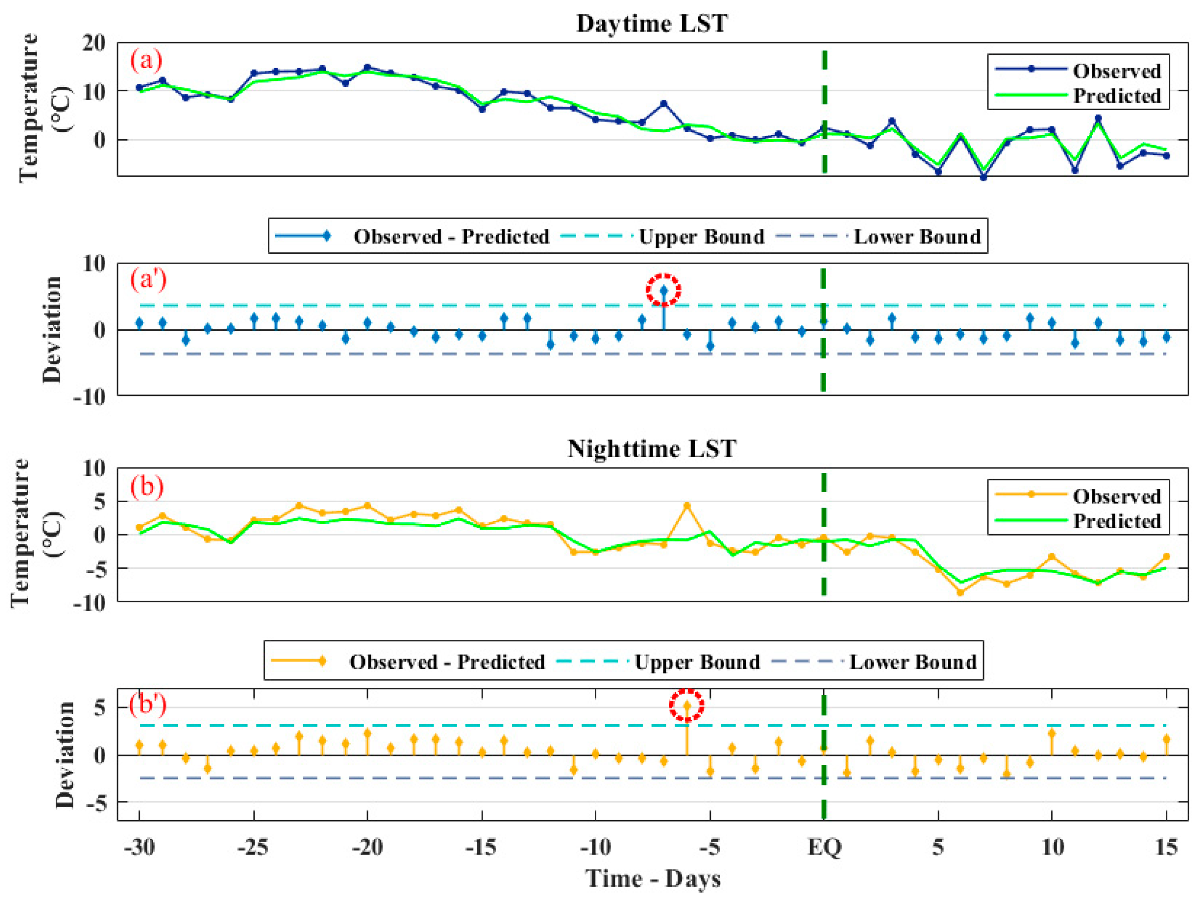
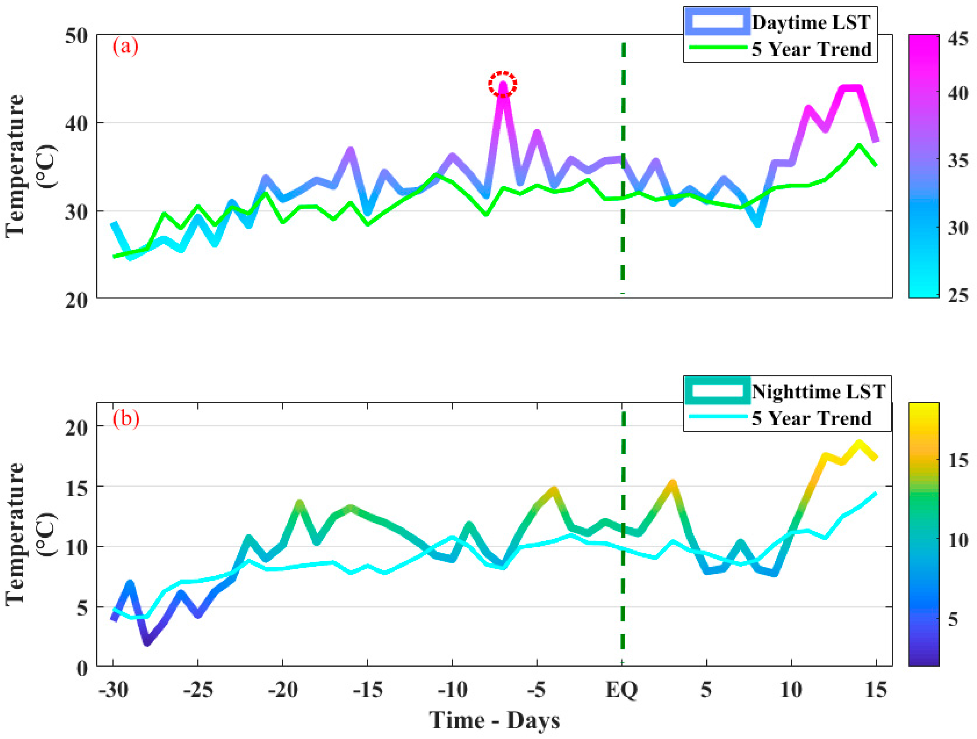
  • The day- and nighttime LST showed a substantial rise of 4 °C and 6 °C in comparison to the 5-year trend within the 5–6 day window prior to the main shock of the Petrolia EQ. The Monte Cristo Range EQ only exhibited a rise in the daytime LST and no substantial increment was visible during the nighttime LST. However, ML analysis revealed the anomalous behavior in the nighttime LST as well in the context of the Monte Cristo Range EQ on the third day before the EQ.
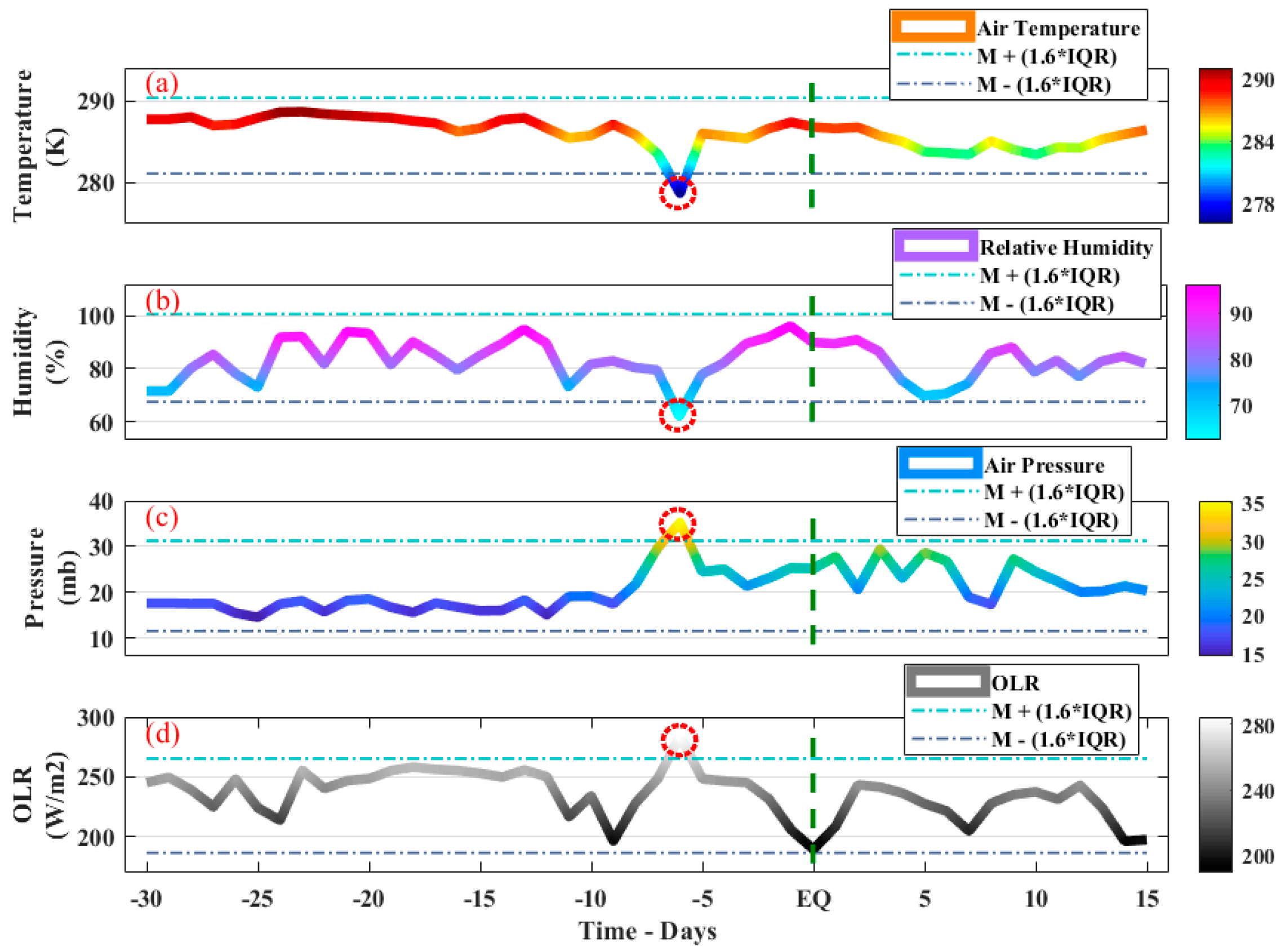
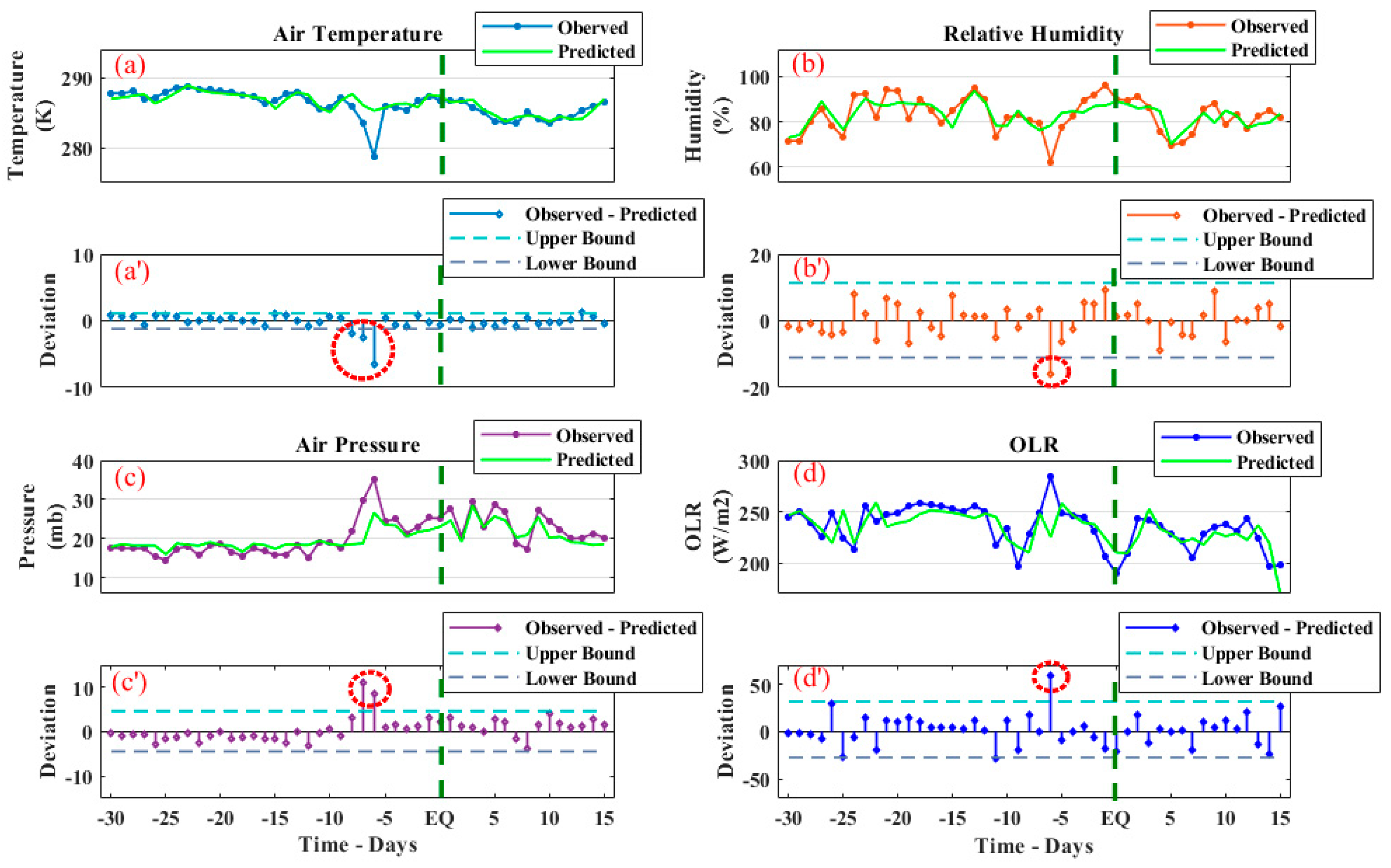
  • A clear drop was observed in the AT on the sixth day prior to the Petrolia EQ and we found this to be seasonal wind composition changes. However, the increment of 13.3 K on the seventh day, in both the statistical and ML analysis for the Monte Cristo Range EQ, confirmed the possible precursors.
  • A prominent anomalous drop of 4% and 8% below the lower bound was observed in RH for both the Petrolia and Monte Cristo Range EQ, respectively. However, ML analysis provided a clear result of the difference between the observed and the predicted RH as 20% and 16% for the Monte Cristo Range and Petrolia EQs, respectively.
  • The AP of the Petrolia EQ exhibited a sharp increase on the sixth day prior to the EQ and no anomaly was visible in the AP of the Monte Cristo Range EQ.
  • Both the statistical and ML analyses provided a similar anomaly date for the OLR on 14th December, about six days before the main shock. Furthermore, a similar pattern was observed by the Monte Cristo Range EQ, but its anomaly occurred on the 8th May for about 7 days before the EQ.
  • The ionosphere TEC exhibited an abrupt variation on a day prior to the EQ in Petrolia region. However, the anomalies in TEC were associated with minor geomagnetic activity. On the other hand, a sudden ionospheric enhancement occurred 6 and 7 days before the preparation period of the Monte Cristo Range EQ in the data of the stations operating inside the Dobrovolsky region, and no anomaly was exhibited by the stations outside the EQ-impacted region.
Our analysis showed clear EQ-induced variations within the 3–7 day window prior to EQs using statistical and ML methods measuring various parameters within the breeding zone. However, we need datasets with better resolution, along with further analysis, in order to forecast EQs in future.

Author Contributions

Conceptualization, M.S.; methodology, software, M.S. and R.S.; writing—review and editing, P.J., B.G., J.F.d.O.-J., A.M.H. and N.A.G. All authors have read and agreed to the published version of the manuscript.

Funding

This research received no external funding.

Institutional Review Board Statement

Not applicable.

Informed Consent Statement

Not applicable.

Data Availability Statement

Not applicable.

Conflicts of Interest

The authors declare no conflict of interest.

References

  1. Tariq, M.A.; Shah, M.; Hernández-Pajares, M.; Iqbal, T. Pre-earthquake ionospheric anomalies before three major earthquakes by GPS-TEC and GIM-TEC data during 2015–2017. Adv. Space Res. 2019, 63, 2088–2099. [Google Scholar] [CrossRef]
  2. Shah, M.; Khan, M.; Ullah, H.; Ali, S. Thermal Anomalies Prior to the 2015 Gorkha (Nepal) Earthquake from Modis Land Surface Temperature and Outgoing Longwave Radiations. Geodyn. Tectonophys. 2018, 9, 123–138. [Google Scholar] [CrossRef] [Green Version]
  3. Khan, M.M.; Ghaffar, B.; Shahzad, R.; Khan, M.R.; Shah, M.; Amin, A.H.; Eldin, S.M.; Naqvi, N.A.; Ali, R. Atmospheric Anomalies Associated with the 2021 Mw 7.2 Haiti Earthquake Using Machine Learning from Multiple Satellites. Sustainability 2022, 14, 14782. [Google Scholar] [CrossRef]
  4. Tronin, A. Remote Sensing and Earthquakes: A Review. Phys. Chem. Earth 2006, 31, 138–142. [Google Scholar] [CrossRef]
  5. Geller, R.J. Special Section—Assessment of Schemes for Earthquake Prediction Earthquake Prediction: A Critical Review. Geophys. J. Int. 1997, 131, 425–450. [Google Scholar] [CrossRef] [Green Version]
  6. Keilis-Borok, V.I.; Soloviev, A.A. Fundamentals of Earthquake Prediction: Four Paradigms. In Nonlinear Dynamics of the Lithosphere and Earthquake Prediction; Springer: Berlin/Heidelberg, Germany, 2003; pp. 1–36. [Google Scholar] [CrossRef]
  7. Shah, M.; Tariq, M.A.; Naqvi, N.A. Atmospheric Anomalies Associated with Mw > 6.0 Earthquakes in Pakistan and Iran during 2010–2017. J. Atmos. Solar-Terr. Phys. 2019, 191, 105056. [Google Scholar] [CrossRef]
  8. Pulinets, S.; Ouzounov, D. The Possibility of Earthquake Forecasting; IOP Publishing: Bristol, UK, 2018; pp. 2–30. [Google Scholar]
  9. Oyama, K.-I.; Kakinami, Y.; Liu, J.Y.; Abdu, M.A.; Cheng, C.Z. Latitudinal Distribution of Anomalous Ion Density as a Precursor of a Large Earthquake. J. Geophys. Res. Atmos. 2011, 116. [Google Scholar] [CrossRef] [Green Version]
  10. Pulinets, S.; Ouzounov, D. Lithosphere-Atmosphere-Ionosphere Coupling (LAIC) Model—An Unified Concept for Earthquake Precursors Validation. J. Asian Earth Sci. 2011, 41, 371–382. [Google Scholar] [CrossRef]
  11. Tariq, M.A.; Yuyan, Y.; Shah, M.; Ali Shah, M.; Iqbal, T.; Liu, L. Ionospheric Thermospheric responses to the May and September 2017 geomagnetic storms over Asian regions. Adv. Space Res. 2022, 70, 3731–3744. [Google Scholar] [CrossRef]
  12. Shah, M.; Ahmed, A.; Ehsan, M.; Khan, M.; Tariq, M.A.; Calabia, A.; Rahman, Z. ur Total Electron Content Anomalies Associated with Earthquakes Occurred during 1998–2019. Acta Astronaut. 2020, 175, 268–276. [Google Scholar] [CrossRef]
  13. Hafeez, A.; Ehsan, M.; Abbas, A.; Shah, M.; Shahzad, R. Machine Learning-Based Thermal Anomalies Detection from MODIS LST Associated with the Mw 7.7 Awaran, Pakistan Earthquake. Nat. Hazards 2022, 111, 2097–2115. [Google Scholar] [CrossRef]
  14. Hafeez, A.; Shah, M.; Naqvi, N.A.; Ehsan, M.; Jamjareegulgarn, P.; Ahmed, J.; Tariq, M.A.; Iqbal, S. Possible Atmosphere and Ionospheric Anomalies of the 2019 Pakistan Earthquake Using Statistical and Machine Learning Procedures on MODIS LST, GPS TEC, and GIM TEC. IEEE J. Sel. Top. Appl. Earth Obs. Remote Sens. 2021, 14, 11126–11133. [Google Scholar] [CrossRef]
  15. Draz, M.U.; Shah, M.; Jamjareegulgarn, P.; Shahzad, R.; Hassan, A.M. Deep Machine Learning based possible Atmospheric and Ionospheric Precursors of the 2021 Mw 7.1 Japan Earthquake. Remote Sens. 2023, 15, 1904. [Google Scholar] [CrossRef]
  16. Khan, A.Q.; Ghaffar, B.; Shah, M.; Ullah, I.; Oliveira-Júnior, J.F.; Eldin, S.M. Possible seismo-ionospheric anomalies associated with the 2016 Mw 6.5 Indonesia earthquake from GPS TEC and Swarm satellites. Front. Astron. Space Sci. 2022, 9, 1065453. [Google Scholar] [CrossRef]
  17. Shah, M.; Abbas, A.; Ehsan, M.; Aiber, A.C.; Adhikari, B.; Tariq, M.A.; Ahmed, J.; de Oliveira-Junior, J.F.; Yan, J.; Morales, A.M.; et al. Ionospheric-Thermospheric Responses to the August 2018 Geomagnetic Storm over South America from Multiple Satellites. IEEE J. Sel. Top. Appl. Earth Obs. Remote Sens. 2021, 15, 261–269. [Google Scholar] [CrossRef]
  18. Pulinets, S.A.; Ouzounov, D.P.; Karelin, A.V.; Davidenko, D.V. Physical Bases of the Generation of Short-Term Earthquake Precursors: A Complex Model of Ionization-Induced Geophysical Processes in the Lithosphere-Atmosphere-Ionosphere-Magnetosphere System. Geomagn. Aeron. 2015, 55, 521–538. [Google Scholar] [CrossRef]
  19. Shah, M.; Jin, S. Pre-Seismic Ionospheric Anomalies of the 2013 Mw = 7.7 Pakistan Earthquake from GPS and COSMIC Observations. Geod. Geodyn. 2018, 9, 378–387. [Google Scholar] [CrossRef]
  20. Shah, M.; Tariq, M.A.; Ahmad, J.; Naqvi, N.A.; Jin, S. Seismo Ionospheric Anomalies before the 2007 M7.7 Chile Earthquake from GPS TEC and DEMETER. J. Geodyn. 2019, 127, 42–51. [Google Scholar] [CrossRef]
  21. Masci, F.; Thomas, J.N. Comment on “Temporal and spatial precursors in ionospheric total electron content of the 16 October 1999 Mw 7.1 Hector Mine earthquake” by Su et al. (2013). J. Geophys. Res. Space Phys. 2014, 119, 6994–6997. [Google Scholar] [CrossRef]
  22. Pulinets, S.A.; Kotsarenko, A.N.; Ciraolo, L.; Pulinets, I.A. Special Case of Ionospheric Day-to-Day Variability Associated with Earthquake Preparation. Adv. Space Res. 2007, 39, 970–977. [Google Scholar] [CrossRef]
  23. Su, Y.C.; Liu, J.Y.; Chen, S.P.; Tsai, H.F.; Chen, M.Q. Temporal and Spatial Precursors in Ionospheric Total Electron Content of the 16 October 1999 Mw7.1 Hector Mine Earthquake. J. Geophys. Res. Space Phys. 2013, 118, 6511–6517. [Google Scholar] [CrossRef]
  24. Kamogawa, M. Preseismic Lithosphere-Atmosphere-Ionosphere Coupling. Eos Trans. Am. Geophys. Union 2006, 87, 417–424. [Google Scholar] [CrossRef] [Green Version]
  25. Freund, F.; Kulahci, I.; Cyr, G.; Ling, J.; Winnick, M.; Tregloan-Reed, J.; Freund, M. Air Ionization at Rock Surface and Pre-Earthquake Signals. J. Atmos. Solar-Terr. Phys. 2009, 71, 1824–1834. [Google Scholar] [CrossRef]
  26. Zhang, Z.-X.; Wang, C.-Y.; Shen, X.-H.; Li, X.-Q.; Wu, S.-G. Study of typical space wave–particle coupling events possibly related with seismic activity. Chin. Phys. B 2014, 23, 109401. [Google Scholar] [CrossRef]
  27. Aleksandrim, S.Y.; Galper, A.M.; Grishantzeva, L.A.; Koldashov, S.V.; Maslennikov, L.V.; Murashov, A.M.; Picozza, P.; Sgrigna, V.; Voronov, S.A. High-energy charged particle bursts in the near-Earth space as earthquake precursors. Ann. Geophys. 2003, 21, 597–602. [Google Scholar] [CrossRef] [Green Version]
  28. Freund, F. Charge Generation and Propagation in Igneous Rocks. J. Geodyn. 2002, 33, 543–570. [Google Scholar] [CrossRef]
  29. Cheng, Y.; Fu, L.-Y. Nonlinear Seismic Inversion by Physics-Informed Caianiello Convolutional Neural Networks for Overpressure Prediction of Source Rocks in the Offshore Xihu Depression, East China. J. Pet. Sci. Eng. 2022, 215, 110654. [Google Scholar] [CrossRef]
  30. Shah, M. Chapter 28—Earthquake Ionospheric and Atmospheric Anomalies from GNSS TEC and Other Satellites. In Computers in Earth and Environmental Sciences; Pourghasemi, H.R.B.T.-C., Ed.; Elsevier: Amsterdam, The Netherlands, 2022; pp. 387–399. ISBN 978-0-323-89861-4. [Google Scholar]
  31. Ouzounov, D.; Pulinets, S.; Romanov, A.; Romanov, A.; Tsybulya, K.; Davidenko, D.; Kafatos, M.; Taylor, P. Atmosphere-Ionosphere Response to the M9 Tohoku Earthquake Revealed by Joined Satellite and Ground Observations. Prelim. Results 2011, 24, 557–564. [Google Scholar]
  32. Shi, K.; Guo, J.; Liu, X.; Liu, L.; You, X.; Wang, F. Seismo-Ionospheric Anomalies Associated with Mw 7.8 Nepal Earthquake on 25 April 2015 from CMONOC GPS Data. Geosci. J. 2020, 24, 391–406. [Google Scholar] [CrossRef]
  33. Thomas, J.N.; Huard, J.; Masci, F. A Statistical Study of Global Ionospheric Map Total Electron Content Changes Prior to Occurrences of M ≥ 6.0 Earthquakes during 2000–2014. J. Geophys. Res. Space Phys. 2017, 122, 2151–2161. [Google Scholar] [CrossRef]
  34. Adil, M.A.; Şentürk, E.; Pulinets, S.A.; Amory-Mazaudier, C. A Lithosphere-Atmosphere-Ionosphere Coupling Phenomenon Observed before M 7.7 Jamaica Earthquake. Pure Appl. Geophys. 2021, 178, 3869–3886. [Google Scholar] [CrossRef]
  35. Pulinets, S.A.; Dunajecka, M.A. Specific Variations of Air Temperature and Relative Humidity around the Time of Michoacan Earthquake M8.1 19 September 1985 as a Possible Indicator of Interaction between Tectonic Plates. Tectonophysics 2007, 431, 221–230. [Google Scholar] [CrossRef]
  36. Ouzounov, D.; Bryant, N.; Logan, T.; Pulinets, S.; Taylor, P. Satellite Thermal IR Phenomena Associated with Some of the Major Earthquakes in 1999–2003. Phys. Chem. Earth 2006, 31, 154–163. [Google Scholar] [CrossRef]
  37. Shah, M.; Ehsan, M.; Abbas, A.; Ahmed, A.; Jamjareegulgarn, P. Possible Thermal Anomalies Associated with Global Terrestrial Earthquakes During 2000–2019 Based on MODIS-LST. IEEE Geosci. Remote Sens. Lett. 2022, 19, 3084930. [Google Scholar] [CrossRef]
  38. Shahzad, R.; Shah, M.; Ahmed, A. Comparison of VTEC from GPS and IRI-2007, IRI-2012 and IRI-2016 over Sukkur Pakistan. Astrophys. Space Sci. 2021, 366, 42. [Google Scholar] [CrossRef]
  39. Dobrovolsky, I.P.; Zubkov, S.I.; Miachkin, V.I. Estimation of the Size of Earthquake Preparation Zones. Pure Appl. Geophys. 1979, 117, 1025–1044. [Google Scholar] [CrossRef]
  40. Mansouri Daneshvar, M.R.; Tavousi, T.; Khosravi, M. Synoptic Detection of the Short-Term Atmospheric Precursors Prior to a Major Earthquake in the Middle East, North Saravan M 7.8 Earthquake, SE Iran. Air Qual. Atmos. Health 2014, 7, 29–39. [Google Scholar] [CrossRef]
  41. Kuo, C.L.; Lee, L.C.; Huba, J.D. An Improved Coupling Model for the Lithosphere-Atmosphere-Ionosphere System. J. Geophys. Res. Space Phys. 2014, 119, 3189–3205. [Google Scholar] [CrossRef]
  42. Pulinets, S.A.; Boyarchuk, K.A. Ionospheric Precursors of Earthquakes; Springer: Berlin/Heidelberg, Germany, 2004. [Google Scholar]
  43. Kiyani, A.; Shah, M.; Ahmed, A.; Shah, H.H.; Hameed, S.; Adil, M.A.; Naqvi, N.A. Seismo ionospheric anomalies possibly associated with the 2018 Mw 8.2 Fiji earthquake detected with GNSS TEC. J. Geodyn. 2020, 140, 101782. [Google Scholar] [CrossRef]
  44. Satti, M.S.; Ehsan, M.; Abbas, A.; Shah, M.; de Oliveira-Júnior, J.F.; Naqvi, N.A. Atmospheric and ionospheric precursors associated with Mw ≥ 6.5 earthquakes from multiple satellites. J. Atmos. Sol. Terr. Phys. 2022, 227, 105802. [Google Scholar] [CrossRef]
  45. Freund, F. Pre-Earthquake Signals: Underlying Physical Processes. J. Asian Earth Sci. 2011, 41, 383–400. [Google Scholar] [CrossRef]
  46. Ouzounov, D.; Freund, F. Mid-Infrared Emission Prior to Strong Earthquakes Analyzed by Remote Sensing Data. Adv. Space Res. 2004, 33, 268–273. [Google Scholar] [CrossRef]
  47. Ouzounov, D.; Liu, D.; Chunli, K.; Cervone, G.; Kafatos, M.; Taylor, P. Outgoing Long Wave Radiation Variability from IR Satellite Data Prior to Major Earthquakes. Tectonophysics 2007, 431, 211–220. [Google Scholar] [CrossRef]
  48. Shahzad, F.; Shah, M.; Riaz, S.; Ghaffar, B.; Ullah, I.; Eldin, S.M. Integrated Analysis of LithosphereAtmosphere-Ionospheric Coupling Associated with the 2021 Mw 7.2 Haiti Earthquake. Atmosphere 2023, 14, 347. [Google Scholar] [CrossRef]
  49. Tuccimei, P.; Mollo, S.; Vinciguerra, S.; Castelluccio, M.; Soligo, M. Radon and Thoron Emission from Lithophysae-Rich Tuff under Increasing Deformation: An Experimental Study. Geophys. Res. Lett. 2010, 37. [Google Scholar] [CrossRef]
  50. Shah, M.; Aibar, A.C.; Tariq, M.A.; Ahmed, J.; Ahmed, A. Possible ionosphere and atmosphere precursory analysis related to Mw > 6.0 earthquakes in Japan. Remote Sens. Environ. 2020, 239, 111620. [Google Scholar]
  51. Freund, F.T.; Takeuchi, A.; Lau, B.W.S.; Al-Manaseer, A.; Fu, C.C.; Bryant, N.A.; Ouzounov, D. Stimulated Infrared Emission from Rocks: Assessing a Stress Indicator. eEarth 2007, 2, 7–16. [Google Scholar] [CrossRef] [Green Version]
  52. Shah, M.; Jin, S. Statistical characteristics of seismo-ionospheric GPS TEC disturbances prior to global Mw ≥ 5.0 earthquakes (1998–2014). J. Geodyn. 2015, 92, 42–49. [Google Scholar] [CrossRef]
  53. Calabia, A.; Anoruo, C.; Shah, M.; Amory-Mazaudier, C.; Yasyukevich, Y.; Owolabi, C.; Jin, S. Low-Latitude Ionospheric Responses and Coupling to the February 2014 Multiphase Geomagnetic Storm from GNSS, Magnetometers, and Space Weather Data. Atmosphere 2022, 13, 518. [Google Scholar] [CrossRef]
  54. Huang, S.; Huang, M.; Lyu, Y. Seismic performance analysis of a wind turbine with a monopile foundation affected by sea ice based on a simple numerical method. Eng. Appl. Comput. Fluid Mech. 2021, 15, 1113–1133. [Google Scholar] [CrossRef]
  55. Huang, S.; Lyu, Y.; Sha, H.; Xiu, L. Seismic performance assessment of unsaturated soil slope in different groundwater levels. Landslides 2021, 18, 2813–2833. [Google Scholar] [CrossRef]
  56. Wu, M.; Ba, Z.; Liang, J. A procedure for 3D simulation of seismic wave propagation considering source-path-site effects: Theory, verification and application. Earthq. Eng. Struct. Dyn. 2022, 51, 2925–2955. [Google Scholar] [CrossRef]
  57. Dang, P.; Cui, J.; Liu, Q.; Li, Y. Influence of source uncertainty on stochastic ground motion simulation: A case study of the 2022 Mw 6.6 Luding, China, earthquake. Stoch. Environ. Res. Risk Assess. 2023, 37, 2943–2960. [Google Scholar] [CrossRef]
  58. Peng, J.; Xu, C.; Dai, B.; Sun, L.; Feng, J.; Huang, Q. Numerical Investigation of Brittleness Effect on Strength and Microcracking Behavior of Crystalline Rock. Int. J. Geomech. 2022, 22, 4022178. [Google Scholar] [CrossRef]
  59. Cheng, F.; Li, J.; Zhou, L.; Lin, G. Fragility analysis of nuclear power plant structure under real and spectrum-compatible seismic waves considering soil-structure interaction effect. Eng. Struct. 2023, 280, 115684. [Google Scholar] [CrossRef]
  60. Zhang, X.; Ma, F.; Dai, Z.; Wang, J.; Chen, L.; Ling, H.; Soltanian, M.R. Radionuclide transport in multi-scale fractured rocks: A review. J. Hazard. Mater. 2022, 424 Pt C, 127550. [Google Scholar] [CrossRef]
  61. Dai, Z.; Ma, Z.; Zhang, X.; Chen, J.; Ershadnia, R.; Luan, X.; Soltanian, M.R. An integrated experimental design framework for optimizing solute transport monitoring locations in heterogeneous sedimentary media. J. Hydrol. 2022, 614, 128541. [Google Scholar] [CrossRef]
  62. Zhang, X.; Wang, Z.; Reimus, P.; Ma, F.; Soltanian, M.R.; Xing, B.; Dai, Z. Plutonium reactive transport in fractured granite: Multi-species experiments and simulations. Water Res. 2022, 224, 119068. [Google Scholar] [CrossRef]
  63. Zhang, Y.; Luo, J.; Zhang, Y.; Huang, Y.; Cai, X.; Yang, J.; Zhang, Y. Resolution Enhancement for Large-Scale Real Beam Mapping Based on Adaptive Low-Rank Approximation. IEEE Trans. Geosci. Remote Sens. 2022, 60, 3202073. [Google Scholar] [CrossRef]
  64. Zhu, W.; Chen, J.; Sun, Q.; Li, Z.; Tan, W.; Wei, Y. Reconstructing of High-Spatial-Resolution Three-Dimensional Electron Density by Ingesting SAR-Derived VTEC into IRI Model. IEEE Geosci. Remote Sens. Lett. 2022, 19, 3178242. [Google Scholar] [CrossRef]
  65. Li, R.; Zhang, H.; Chen, Z.; Yu, N.; Kong, W.; Li, T.; Liu, Y. Denoising method of ground-penetrating radar signal based on independent component analysis with multifractal spectrum. Measurement 2022, 192, 110886. [Google Scholar] [CrossRef]
  66. Zhuo, Z.; Du, L.; Lu, X.; Chen, J.; Cao, Z. Smoothed Lv Distribution Based Three-Dimensional Imaging for Spinning Space Debris. IEEE Trans. Geosci. Remote Sens. 2022, 60, 3174677. [Google Scholar] [CrossRef]
  67. Liu, H.; Yue, Y.; Liu, C.; Spencer, B.F.; Cui, J. Automatic recognition and localization of underground pipelines in GPR B-scans using a deep learning model. Tunn. Undergr. Space Technol. 2023, 134, 104861. [Google Scholar] [CrossRef]
  68. Liu, H.; Li, J.; Meng, X.; Zhou, B.; Fang, G.; Spencer, B.F. Discrimination between Dry and Water Ices by Full Polarimetric Radar: Implications for China’s First Martian Exploration. IEEE Trans. Geosci. Remote Sens. 2022, 61, 3228684. [Google Scholar] [CrossRef]
  69. Zhan, C.; Dai, Z.; Soltanian, M.R.; de Barros FP, J. Data-worth analysis for heterogeneous subsurface structure identification with a stochastic deep learning framework. Water Resour. Res. 2022, 58, e2022WR033241. [Google Scholar] [CrossRef]
  70. Liu, W.; Zhou, H.; Zhang, S.; Zhao, C. Variable Parameter Creep Model Based on the Separation of Viscoelastic and Viscoplastic Deformations. Rock Mech. Rock Eng. 2023, 56, 4629–4645. [Google Scholar] [CrossRef]
  71. Bai, B.; Zhou, R.; Cai, G.; Hu, W.; Yang, G. Coupled thermo-hydro-mechanical mechanism in view of the soil particle rearrangement of granular thermodynamics. Comput. Geotech. 2021, 137, 104272. [Google Scholar] [CrossRef]
  72. Hou, X.; Zhang, L.; Su, Y.; Gao, G.; Liu, Y.; Na, Z.; Chen, T. A space crawling robotic bio-paw (SCRBP) enabled by triboelectric sensors for surface identification. Nano Energy 2023, 105, 108013. [Google Scholar] [CrossRef]
  73. Zheng, Z.; Zuo, Y.; Wen, H.; Li, D.; Luo, Y.; Zhang, J.; Zeng, J. Natural gas characteristics and gas-source comparisons of the lower Triassic Feixianguan formation, Eastern Sichuan basin. Pet. Sci. 2023, 20, 1458–1470. [Google Scholar] [CrossRef]
  74. Zhou, G.; Zhou, X.; Song, Y.; Xie, D.; Wang, L.; Yan, G.; Wang, H. Design of supercontinuum laser hyperspectral light detection and ranging (LiDAR) (SCLaHS LiDAR). Int. J. Remote Sens. 2021, 42, 3731–3755. [Google Scholar] [CrossRef]
  75. Zhou, G.; Li, W.; Zhou, X.; Tan, Y.; Lin, G.; Li, X.; Deng, R. An innovative echo detection system with STM32 gated and PMT adjustable gain for airborne LiDAR. Int. J. Remote Sens. 2021, 42, 9187–9211. [Google Scholar] [CrossRef]
  76. Zhou, G.; Deng, R.; Zhou, X.; Long, S.; Li, W.; Lin, G.; Li, X. Gaussian Inflection Point Selection for LiDAR Hidden Echo Signal Decomposition. IEEE Geosci. Remote Sens. Lett. 2021, 19, 3107438. [Google Scholar] [CrossRef]
  77. Zhou, L.; Ye, Y.; Tang, T.; Nan, K.; Qin, Y. Robust Matching for SAR and Optical Images Using Multiscale Convolutional Gradient Features. IEEE Geosci. Remote Sens. Lett. 2022, 19, 3105567. [Google Scholar] [CrossRef]
  78. Yue, Z.; Zhou, W.; Li, T. Impact of the Indian Ocean Dipole on Evolution of the Subsequent ENSO: Relative Roles of Dynamic and Thermodynamic Processes. J. Clim. 2021, 34, 3591–3607. [Google Scholar] [CrossRef]
  79. Xu, Z.; Wang, Y.; Jiang, S.; Fang, C.; Liu, L.; Wu, K.; Chen, Y. Impact of input, preservation and dilution on organic matter enrichment in lacustrine rift basin: A case study of lacustrine shale in Dehui Depression of Songliao Basin, NE China. Mar. Pet. Geol. 2022, 135, 105386. [Google Scholar] [CrossRef]
  80. Li, C.; Smith, P.; Bai, X.; Tan, Q.; Luo, G.; Li, Q.; Zhang, S. Effects of carbonate minerals and exogenous acids on carbon flux from the chemical weathering of granite and basalt. Glob. Planet. Chang. 2023, 221, 104053. [Google Scholar] [CrossRef]
  81. Wei, X.; Bai, X.; Wen, X.; Liu, L.; Xiong, J.; Yang, C. A large and overlooked Cd source in karst areas: The migration and origin of Cd during soil formation and erosion. Sci. Total Environ. 2023, 895, 165126. [Google Scholar] [CrossRef]
  82. Chen, J.; Wen, L.; Bi, C.; Liu, Z.; Liu, X.; Yin, L.; Zheng, W. Multifractal analysis of temporal and spatial characteristics of earthquakes in Eurasian seismic belt. Open Geosci. 2023, 15, 20220482. [Google Scholar] [CrossRef]
  83. Yin, L.; Wang, L.; Ge, L.; Tian, J.; Yin, Z.; Liu, M.; Zheng, W. Study on the Thermospheric Density Distribution Pattern during Geomagnetic Activity. Appl. Sci. 2023, 13, 5564. [Google Scholar] [CrossRef]
Figure 1. Geographical locations of the study area with the red star for the EQs epicenters. The ellipses show the impacted area and the GNSS stations are represented by the blue stars.
Atmosphere 14 01236 g001
Figure 2. The flow chart of the NARX time series data prediction.
Atmosphere 14 01236 g002
Figure 3. The LST time series of the Petrolia EQ. (a) Daytime series from 20 November 2021 to 4 January 2022 with the past 5 years of the same days from 2016 to 2020, and (b) nighttime data from 20 November 2021 to 4 January 2022 with the past 5 years of the same nights from 2016 to 2020. The red dotted area indicates the anomalous variations. The EQ time is indicated by a vertical green dotted line.
Atmosphere 14 01236 g003
Figure 4. The comparison plot between the observed and the NARX predicted LST. (a) Daytime LST time series, (b) deviation between the retrieved and predicted LST, (a’) the observed and predicted LST of nighttime, and (b’) the nighttime MODIS LST from the NARX predicted LST. The EQ is indicated by a vertical green dotted line and the red dotted line represents the observed anomaly.
Atmosphere 14 01236 g004
Figure 5. The variations in the atmospheric parameters of the Petrolia EQ. (a) Air Temperature, (b) Relative Humidity, (c) Air Pressure, and (d) Outgoing Longwave Radiations. The red dotted area indicated the anomalous variations. The EQ is indicated by a vertical green dotted line. The * sign is used as multiplication symbol.
Atmosphere 14 01236 g005
Figure 6. The variations between the observed and the NARX predicted atmospheric parameters. (ad) show comparison of AT, RH, AP and OLR, respectively; whereas, (a’d’) are the deviations between the observed AT, RH, AP and OLR and the NARX predicted values of these atmospheric parameters. The EQ time is indicated by a vertical green dotted line and the red dotted circle is the anomaly.
Atmosphere 14 01236 g006
Figure 7. The ionospheric variations from TEC and the geomagnetic storm activities for 30 days before and 15 days after the main shock of the Petrolia EQ. (a,b) The geomagnetic storm indices as Dst and Kp, (c) GNSS stations within the EQ impacted region and (df) GNSS stations outside the EQ impacted region. The EQ time is indicated by a vertical green dotted line.
Atmosphere 14 01236 g007
Figure 8. The TEC variations between the GNSS stations retrieved TEC and the NARX predicted TEC in (a) P389, (b) COSO, (c) DRAO and (d) HOLB GNSS stations. Furthermore, the P389 station is located inside the Dobrovolsky region. (e) The deviation between the observed TEC and the NARX predicted TEC of all the stations. The EQ time is indicated by a vertical green dotted line and the storm anomaly is indicated by a red dashed circle.
Atmosphere 14 01236 g008
Figure 9. The LST time series graph of the Monte Cristo Range EQ (Mw 6.5 occurred on 15 May 2020) along with the 5-year trend for the same days from 2015 to 2019 over same region for; (a) the daytime LST, and (b) the nighttime LST. The red dotted area indicates the anomalous variations. The EQ time is indicated by a vertical green dotted line.
Atmosphere 14 01236 g009
Figure 10. The LST variations of the MODIS retrieved LST and the NARX predicted LST as (a) the daytime LST and (b) the nighttime LST pattern from the MODIS original analysis and the NARX observed day- and nighttime. (a’) The deviations between observed the daytime LST and daytime NARX predicted LST and (b’) the deviations between the nighttime observed LST and the nighttime NARX predicted LST. The EQ time is indicated by a vertical green dotted line.
Atmosphere 14 01236 g010
Figure 11. The variations in atmospheric parameters for the Monte Cristo Range EQ within the confidence bounds. (a) Air Temperature, (b) Relative Humidity, (c) Air Pressure, and (d) Outgoing Longwave Radiations. The red dotted area indicates anomalous variations. The EQ time is indicated by a vertical green dotted line. The * sign is used as multiplication symbol.
Atmosphere 14 01236 g011
Figure 12. The time series variations between the observed and the NARX predicted atmospheric parameters, where (a) represents the observed and predicted AT and (a’) is the deviations between the observed AT and predicted AT. (b) The observed RH and the predicted RH and (b’) is the deviation between the observed and their predicted RH. (c) is for the time series of the retrieved AP and NARX AP and (c’) is the deviation between the predicted values of AP and observed values of AP. (d) is the comparison graph of the observed OLR and predicted OLR and (d’) is the predicted OLR deviation from the observed OLR. The EQ time is indicated by a vertical green dotted line.
Atmosphere 14 01236 g012
Figure 13. The ionospheric TEC and geomagnetic activity variations for 30 days before and 15 days after the Monte Cristo Range EQ. (a) Kp, (b) Dst, (c,d) GNSS stations within the EQ impacted region, and (e,f) GNSS stations outside the EQ impacted region. The EQ day is shown by a green dashed line.
Atmosphere 14 01236 g013
Figure 14. The variations between the GNSS stations retrieved from GNSS TEC and NARX predicted TEC. (ad) GNSS stations TEC and the NARX predicted TEC from COSO and QUIN stations inside the Dobrovolsky region, but DRAO and HOLB are outside the EQ preparation zone. (e) The deviation between the observed TEC and NARX predicted TEC for all the stations. The EQ time is indicated by a vertical green dotted line.
Atmosphere 14 01236 g014
Figure 15. An illustration of the LAIC hypothesis and the corresponding anomalies that occurred in the satellite data in this study.
Atmosphere 14 01236 g015
Table 1. GNSS stations used for TEC retrieval.
GNSS Station NameInside Dobrovolsky RegionOutside Dobrovolsky Region
PetroliaMonte Cristo RangePetroliaMonte Cristo Range
P389
COSO
QUIN
DRAO
HOLB
Disclaimer/Publisher’s Note: The statements, opinions and data contained in all publications are solely those of the individual author(s) and contributor(s) and not of MDPI and/or the editor(s). MDPI and/or the editor(s) disclaim responsibility for any injury to people or property resulting from any ideas, methods, instructions or products referred to in the content.

