The Spatio-Temporal Cloud Frequency Distribution in the Galapagos Archipelago as Seen from MODIS Cloud Mask Data

Abstract

Clouds play an important role in the climate system; nonetheless, the relationship between climate change in general and regional cloud occurrence is not yet well understood. This particularly holds for remote areas such as the iconic Galapagos archipelago in Ecuador. As a first step towards a better understanding, we analyzed the spatio-temporal patterns of cloud cover over Galapagos. We found that cloud frequency and distribution exhibit large inter- and intra-annual variability due to the changing influence of climatic drivers (trade winds, sea surface temperature, El Niño/La Niña events) and spatial variations due to terrain characteristics and location within the archipelago. The highest cloud frequencies occur in mid-elevations on the slopes exposed to the southerly trade winds (south-east slopes). Towards the highlands ( >900 m a.s.l), cloud frequency decreases, with a sharp leap towards high-level crater areas mainly on Isabela Island that frequently immerse into the trade inversion layer. With respect to the diurnal cycle, we found a lower cloud frequency over the islands in the evening than in the morning. Seasonally, cloud frequency is higher during the hot season (January–May) than in the cool season (June–December). However, spatial differences in cloudiness were more pronounced during the cool season months. We further analyzed two periods beyond average atmospheric forcing. During El Niño 2015, the cloud frequency was higher than usual, and differences between altitudes and aspects were less pronounced. La Niña 2007 led to negative anomalies in cloud frequency over the islands, with intensified differences between altitude and aspect.

1. Introduction

The remote Galapagos archipelago is known for its unique biodiversity and endemic species. The local climate is the result of a complex interplay between different climatic drivers such as different ocean currents (e.g., Equatorial Undercurrent west of the archipelago, Humboldt Current south-east of the archipelago), the seasonal shift in the Inter-Tropical Convergence Zone (ITCZ), and the quasi-periodic El Niño Southern Oscillation (ENSO) phenomenon [1,2,3]. This finely balanced system is sensitive to any external impact, such as global warming, which could have a major adverse effect on this globally unique ecosystem. Hence, the archipelago is considered one of the most vulnerable places in terms of climate change, especially considering its great (endemic) biodiversity [1,2,3,4].

One of the biggest challenges in forecasting future climate is accurately understanding the relationship between clouds and global warming. Uncertainties are, to date, largely due to the complicated interplay of numerous feedback mechanisms between climate and clouds, which are still not fully understood ([5], p. 926). Cloud properties such as amount, distribution, height, and occurrence time determine how strong and in which way clouds modify the global energy budget [6,7,8]. On the other hand, climate affects the conditions under which clouds form and, therefore, determines their properties, such as the spatial distribution and composition, but also their properties concerning radiation and hydrology (e.g., water content) which, in turn, lead to a modification of the climate [9]. Since the role of clouds in the climate system is so significant but not yet fully understood, it is important to conduct further research, particularly in understudied remote regions such as the Galapagos archipelago [10,11].

Here, the knowledge about clouds is especially important for the precious ecosystem, as they play an important role in the water supply of the archipelago. Without clouds, there can not be any precipitation. Convective precipitation on Galapagos occurs mainly during the period from January to May. During the rest of the year, the water supply relies on drizzle and occult precipitation that results from Garúa, a fog that regularly occurs in the high-altitude areas of the islands [12]. Garúa serves as an important source of water for the plants and ecosystems in the highlands, where it is the main driver of vegetation productivity [12,13,14]. Moreover, Garúa is also a potential source of freshwater [15,16], which will become even more important with the increase in population and tourism. Despite its ecological and socio-economic importance, studies of Garúa have so far only focused on single location and islands. Even less is known about the local occurrence and spatio-temporal distribution of clouds in general for the Galapagos archipelago.

Commonly used methods to study clouds rely on remote sensing, as it provides area-wide information in high spatio-temporal resolution and obtains its data directly from the clouds. There have been several studies that used satellite data to investigate cloud frequency over different regions of the earth, such as the Peruvian Andes [17], the United States mainland [6], Hawaii [18], or the mainland of Ecuador [19]. Even though the studies differed in their details, they all showed that the terrain influences the pattern of cloud distribution. Higher cloud occurrence is found on wind-facing slopes. In addition, strong influences on diurnal and seasonal changes in spatial cloud distribution were also found. In the study for mainland Ecuador, based on NOAA-AVHRR data, the Andes Mountains proved to be a barrier dividing the country into a western part with lower cloud patterns from the Pacific and more convective cloud patterns on the eastern slopes towards the Amazon. This general cloud zonation is locally modified by mesoscale systems (sea and mountain winds, etc.) [19]. In Hawaii, analysis of 11 years of MODIS cloud mask data revealed that the trade winds play a leading role in explaining cloud distribution. Thus, the highest cloud frequencies were found on windswept mountain slopes at elevations between the upwelling condensation level and the trade wind inversion base [18]. Considering the governing factors of the climate in the Galapagos archipelago, including the ITCZ, a well-developed land–sea breeze system, and the quasi-periodic ENSO phenomenon, along with elevations exceeding 1700 $\mathrm{m}$ a.s.l, the nature on the spatial distribution of clouds remains unclear. So far, no study of cloud distribution was performed for Galapagos.

This study systematically investigates the cloud frequency over the archipelago in space and time using the Moderate Resolution Imaging Spectrometer (MODIS) cloud mask data. The paper is organized as follows. Section 2 gives a brief overview of the study area and its local climate drivers (Section 2.1). It also introduces the used data (Section 2.2 and Section 2.3) and the applied methods (Section 2.4, Section 2.5, Section 2.6, Section 2.7). The results are presented in Section 3, where we focus on the analysis of diurnal and spatial distribution patterns in the cloud frequency in Section 3.1, the intra-annual variation due to the seasonality in Section 3.2, and the inter-annual variations caused by ENSO in Section 3.3. All results are discussed in Section 4. We summarize our study and present our conclusions in Section 5.

2. Data & Methods

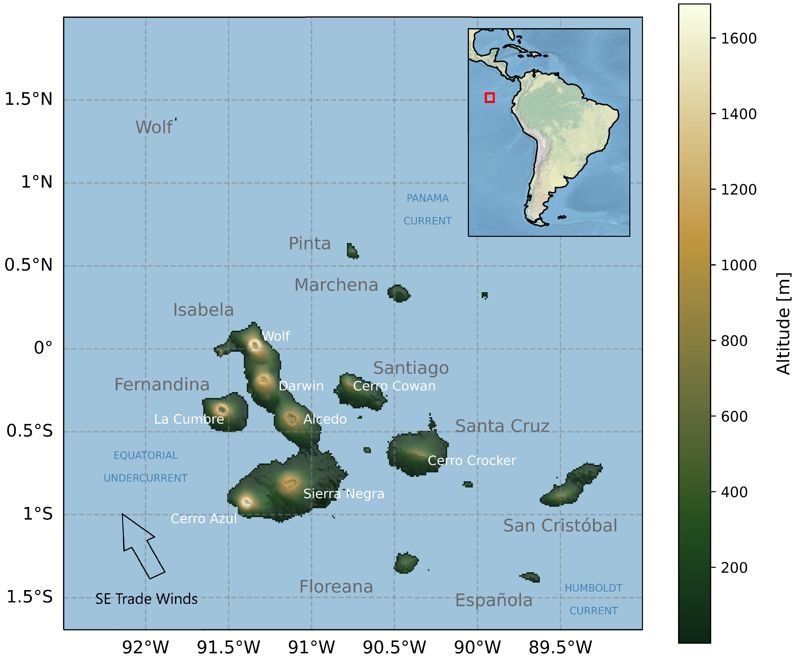
2.1. Study Area

The Galapagos Islands are located around 1000 km west of the Ecuadorian mainland, in the eastern, tropical Pacific Ocean, spanning from $89.0°$ W to $-92.5°$ W and $2.0°$ N to $-1.7°$ S. The archipelago consists of about 130 islands, but only 13 of them exceed an area of 10 km². Galapagos was formed and continues to be shaped by volcanic eruptions. With an altitude of 1707 $\mathrm{m}$ a.s.l., the volcano Volcán Wolf, located on the largest island Isabela, represents the highest elevation on the archipelago (Figure 1). The topography has a strong influence on the local climate and, therefore, also on the vegetation. Based on the climatic conditions, three different zones can be identified: dry lowlands, humid highlands, and dry uplands [12].

The combination of multiple oceanic currents, the movement of the ITCZ, and trade winds leads to an atypical climate for the geographical region of the Galapagos Islands [15]. Three major ocean currents meet in the Galapagos: the warm Panama Current from the north, the cold Humboldt Current from the south-east, and the upwelling of the cold Pacific Undercurrent to the west of the archipelago [3]. The annual shift of the ITCZ, between 10° N and 3° S, has a big influence on the climate of the archipelago and leads to the formation of two different seasons [12,14]. The so-called cool season, which lasts from June to December, is characterized by strong trade winds, blowing from the south-east [20]. During this phase, the ITCZ is shifted to the north so that the trade winds at Galapagos are stronger [12,20,21]. As a result, the air, transported by the trade winds, cools while passing the cold oceanic surface [12]. This leads to an inversion, by which the cold air is trapped under the warmer layer of air. Above this inversion base, cloud formation is clearly reduced. When hitting the islands, the air is forced to rise and condensation forms low stratus clouds right under the inversion layer [14]. The stratus clouds often reach the ground and lead to fog and heavy mist, which is locally called Garúa [3,12,14]. Garúa is reported to occur generally above an altitude of 250 $\mathrm{m}$ and results in two types of precipitation: very light rainfall (drizzle) and occult precipitation (cloud-water combing and deposition) [12]. In contrast, the warm or hot season (January to May) is characterized by higher temperatures [15]. The ITCZ is located in the southward position near the Galapagos Islands [12]. This affects the trade winds, which blow only weakly above the archipelago [15]. During this time, convective rainfall dominates the precipitation [12]. These annual variations are superimposed by ENSO, which takes place every 2–7 years and typically lasts 1–1.5 years [22,23]. On the Galapagos Islands, the El Niño phenomenon is noticeable through higher air and sea surface temperatures as well as weakened trade winds [14,24]. This weakens the inversion layer of the cool season and facilitates the development of heavy convective rainfalls and an extended hot season [12,24,25]. In contrast, La Niña is characterized by weather conditions that are colder and drier than normal [14]. During this time, the trade winds are particularly strong [24].

An overview of the climate in the Galapagos is provided in Figures S2 and S3 by visualizing the data from four weather stations located within the Archipelago (locations: Figure S1, Table S1). The monthly and seasonal wind statistics are additionally depicted in Figures S4–S6.

2.2. MODIS Cloud Mask Data

To obtain the relative cloud frequency, the level 2 satellite product of MODIS/Terra Cloud Mask (MOD35) [26] was used. The MODIS is an instrument on the National Aeronautics and Space Administration (NASA) satellite Terra. MODIS has 36 spectral bands to detect electromagnetic waves in the wavelength range of $0.7$ $\mu$$\mathrm{m}$ to $14.2$ $\mu$$\mathrm{m}$ [27,28]. From the raw data, the cloud mask algorithm is used to determine the existence of the clouds for each pixel. This algorithm is based on the feature that clouds have a higher reflectance and a lower temperature than the earth’s surface [28]. To detect these differences, data from 19 spectral bands are used [28]. The clouds are identified by applying different threshold tests. The performed tests depend on the region, the earth’s surface (e.g., ocean, vegetated and desert surfaces) and the sunlight [27,28]. Each test leads to a confidence level that a cloud is detected, which are in the end combined to a final cloud mask flag [27,28]. This flag classifies each pixel to one of the four levels: confident clear, probably clear, uncertain clear and cloudy [27,28]. The used cloud mask data originates from the period from 25 February 2000 to 31 December 2021 and has a spatial resolution of 1000 $\mathrm{m}$ × 1000 $\mathrm{m}$ (at the nadir). The Terra satellite crosses the study area two times per day. The first overflight takes place in the morning between 9:20 and 11:45 local time, and the second overflight occurs between 21:20 and 23:40. In the following, these two sets of data are referred to as the morning and evening overflights, respectively. The total number of processed cloud product scenes was 33,053.

2.3. Terrain Data

Knowledge about the elevation and the aspect of the islands was gained using the Advanced Spaceborne Thermal Emission and Reflection Radiometer (ASTER) global digital elevation model [29]. The terrain data, with the original spatial resolution of 30 $\mathrm{m}$, were resampled to the same grid as the cloud frequency data, by using the nearest neighbor method. Based on the elevation model, the aspect (orientation of each terrain pixel) was determined.

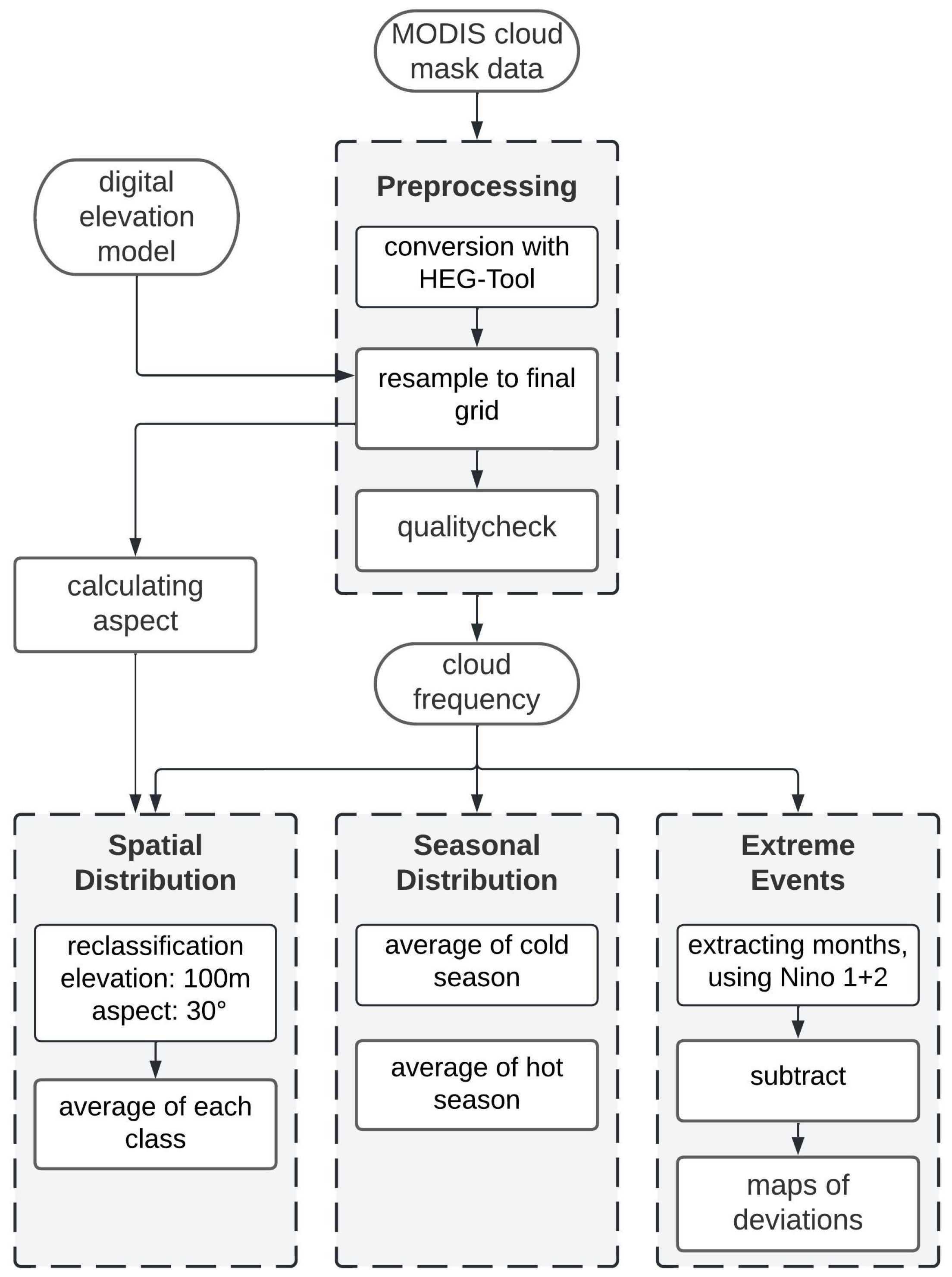
2.4. Data Processing

The work process is shown schematically in Figure 2. The steps of the data preprocessing are summarized in the upper box of the flowchart. After downloading the MODIS Cloud Mask data from the website https://search.earthdata.nasa.gov/ (accessed on 17 January 2022), the files were converted from HDF to NetCDF and projected using the NASA HDF-EOS to GeoTIFF Converter (HEG) tool [30] (downloaded via https://wiki.earthdata.nasa.gov/display/DAS/Downloads, accessed on 20 November 2021). The data were projected to World Geodetic System 1984 (WGS 84) using geographical projection and resampled to a final $0.009°$ × $0.009°$ ( 1 × 1 ) grid using the nearest neighbor method. All steps were conducted in Python.

After gaining access to the data, the preprocessing path proposed in the MODIS Cloud Mask User Guide [31] was followed to ensure that only data of sufficient quality were used in this analysis. Since the information was saved in a 48-bit mask, the data had to be decoded bitwise. First, the included quality assurance (QA) data set was evaluated. Each QA flag provides information about the quality of the cloud mask or the application of a specific test or processing path. Only pixels with the cloud mask flag set to “determined” were included in further processing. If the QA flag of the cloud mask was set to “not useful”, the pixel was excluded. For the evening overpass, it was checked if the QA flag was set to “nighttime”, and, for the morning overpass, to “daytime”. For easier handling, the remaining data were reclassified from the original four categories (cloudy, uncertain clear, probably clear, confident clear) in two categories: “cloudy” and “clear”. The new category “cloudy” included the old categories “cloudy” and “uncertain clear”, and the new category “clear” combined the two old categories “probably clear” and “confident clear”.

2.5. Cloud Frequency Analysis

From the preprocessed data, the relative cloud frequency was calculated for each month, which allowed us to handle the big amount of data analyzed in this study. Therefore, the number of days on which the pixel was declared as “cloudy” was divided by the number of days for which usable data were available (

Table 1. Overview of used methods and formulas. Calculations were carried out pixelwise. To quantify the differences in cloud frequency caused by ENSO, a comparison period to the ENSO period was defined. This comparison period consisted of the long-term averages of the same months as the ENSO event.

Data Set	Formula	Value Range
monthly relative cloud frequency	$\frac{\sum \mathrm{cloud} \mathrm{mask} \mathrm{values} \mathrm{of} \mathrm{month}}{\# \mathrm{available} \mathrm{days} \mathrm{of} \mathrm{month}}$	0: all days clear sky 1: all days clouds
hot season cloud frequency	$\frac{\sum \mathrm{monthly}\mathrm{rel}.\mathrm{cloud}\mathrm{frequency}(\mathrm{January}\mathrm{to}\mathrm{May})}{\# \mathrm{months} (\mathrm{January} \mathrm{to} \mathrm{May})}$	0: all days clear sky 1: all days clouds
cool season cloud frequency	$\frac{\sum \mathrm{monthly}\mathrm{rel}.\mathrm{cloud}\mathrm{frequency}(\mathrm{June}\mathrm{to}\mathrm{December})}{\# \mathrm{months} (\mathrm{June} \mathrm{to} \mathrm{December})}$	0: all days clear sky 1: all days clouds
general relative cloud frequency	$\frac{\sum \mathrm{monthly}\mathrm{cloud}\mathrm{frequency}}{\# \mathrm{months}}$	0: all days clear sky 1: all days clouds
deviation of extreme events	$$\begin{gathered} \frac{\sum \mathrm{monthly}\mathrm{cloud}\mathrm{frequency}(\mathrm{ENSO}\mathrm{event})}{\# \mathrm{months} (\mathrm{ENSO} \mathrm{event})}- \\ \frac{\sum \mathrm{monthly}\mathrm{cloud}\mathrm{frequency}(\mathrm{comparison}\mathrm{period})}{\# \mathrm{months} (\mathrm{comparison} \mathrm{period})} \end{gathered}$$	>0: more clouds during ENSO <0: less clouds during ENSO

). Thus, the relative cloud frequency ranged between 0 and 1, where 1 meant each day was cloudy, and 0 meant that all days were clear. The general relative cloud frequency was calculated by averaging the monthly data sets over the entire time period so that, for each pixel, the average value of cloud occurrence over the time period was obtained. The relative cloud frequency per season was calculated by splitting the general data set into two sets, one for the hot season (January to May) and the other for the cool season (June to December). This followed the common definition of the two seasons as given, for example, by Trueman and d’Ozouville [12], Sachs and Ladd [14]. Averaging these two seasonal data sets individually led to the relative cloud frequency for the hot and cool seasons. The whole process was executed for the morning and for the evening overpass.

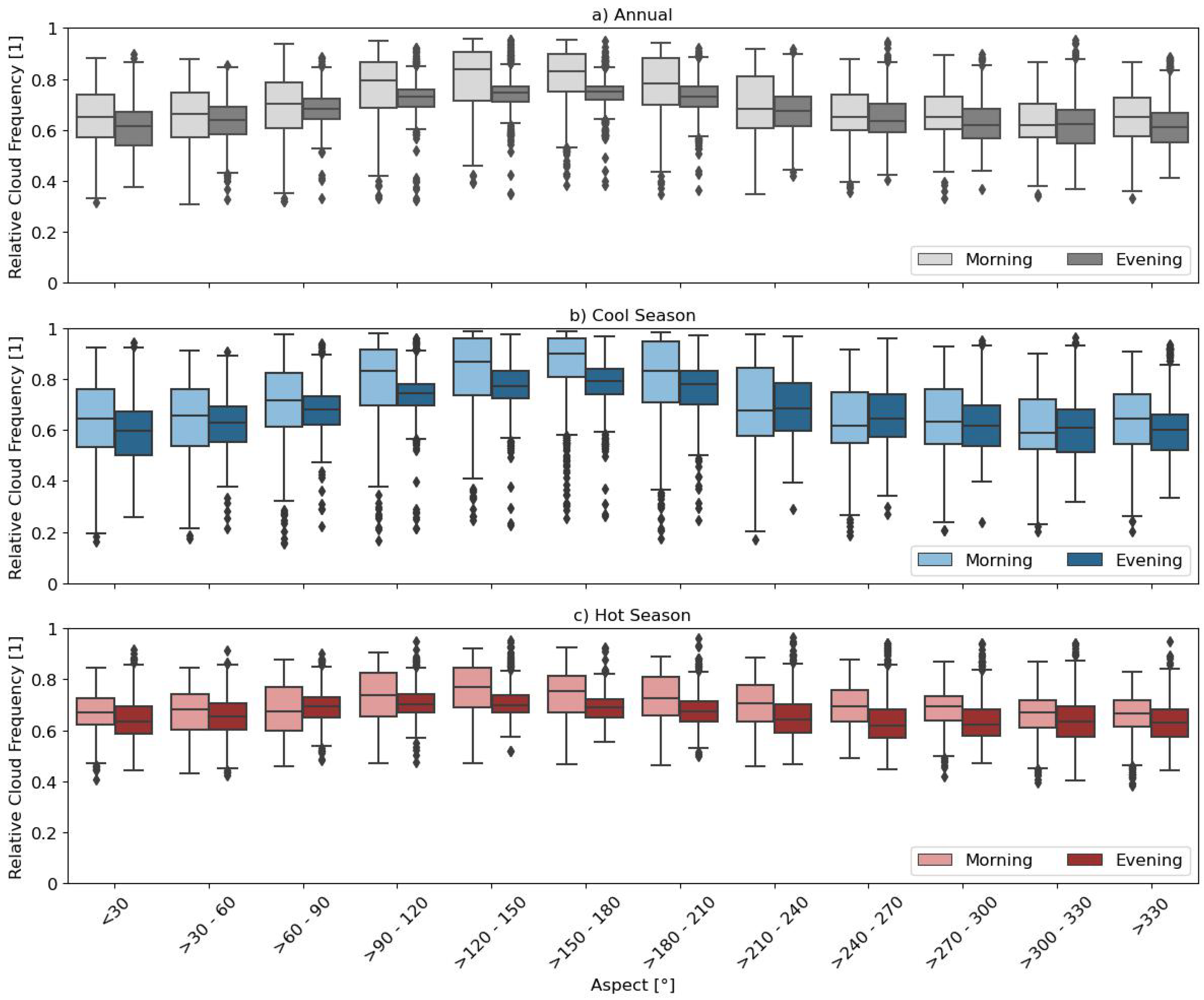
2.6. Cloud Frequency Analysis along Elevation and Aspect

In order to determine the dependence of the relative cloud frequency on the terrain altitude and the terrain aspect, the rasterized digital elevation model was used. The terrain data were reclassified in classes of 100 $\mathrm{m}$ elevation. From all pixels included in the particular group, a box plot of the corresponding relative cloud frequency was created. The same procedure was repeated with the terrain aspect. Here, each class consisted of data for a range of 30°. A specific class (e.g., >120°–210°) thus included all pixels exceeding the minimum threshold while being less than or equal to the maximum threshold, whereby, e.g., >120° means $120.1°$. For both analyses, only land pixels (elevation $>0$ $\mathrm{m}$) were used. In order to analyze the diurnal variation in cloud frequency, the results of the morning and evening overflights were compared.

To identify which of the two factors, elevation or aspect, is more important for the spatial distribution of the clouds, a random forest regression was performed. This method was chosen because the dependence of relative cloud frequency on terrain height and terrain aspect could not be described sufficiently by linear, quadratic, or polynomial regression. The random forest regression was proposed by Breiman [32] and is a nonparametric machine learning model. Within the random forest regression, multiple decision trees are trained on a random subset of the training data. The final result of the regression is the output mean of the multiple decision trees. The importance of a feature within the random forest can be quantified by the Gini importance [33]. The Gini importance measures the average reduction in node impurity for a variable. This reduction is weighted by the proportion of samples that reach that node in each individual decision tree within the random forest [34]. The higher the value of a feature, the higher its importance (value range: 0 to 1).

To perform the random forest regression, the python-package Scikit-Learn [33] was used. The initial data set, the cloud frequency as a function of elevation and aspect, was randomly divided into a training and a test data set. The training data set comprised 75% of the total data. The feature importance was determined by applying the built-in function “feature_importance_” of the class “RandomForestRegressor” in the Scikit-Learn package.

2.7. Cloud Frequency Analysis in Extreme Events

According to the definition of NOAA (National Oceanic and Atmospheric Administration) [35], an ENSO event takes place when the deviation of the Oceanic Niño Index (ONI) exceeds a threshold of $\pm 0.5 °\mathrm{C}$. The ONI is the mean of the sea surface temperature (SST) of three consecutive months in the Niño 3.4 region, which is located in the central Pacific (5° N–5° S, 120°–170° W) [35]. Since Conroy et al. [36] showed that the correlation between the Niño 1 + 2 index and the climate on Galapagos is stronger than the correlation to Niño 3.4, this index was used to define the temporal boundaries of the ENSO events. The Niño 1 + 2 region considers the anomalies of the SST in the tropical Pacific in the area 0° S–10° S and 90° W–80° W; Galapagos is located on this region’s edge. The effect of ENSO events on cloud frequency was examined in this study using the El Niño event 2015 and the La Niña event 2007 as examples, since these two events had the strongest SST anomalies in the Niño 1 + 2 region (Table S2). For the El Niño event in 2015, months with an SST anomaly of Niño 1 + 2 $>1.5$ $°\mathrm{C}$ were included. This led to the temporal limitation of the event to the duration from May 2015 to January 2016. For the analyzed La Niña event in 2007, the months April 2007 to December 2007 were included. All these months had SST anomalies <−0.9 $°\mathrm{C}$. We analyzed the deviation in cloud frequency during these events as follows. For each month of the events, the relative cloud frequency was calculated. Subsequently, the mean values for each month were also calculated over the whole time period. This resulted in one “normal” comparison data set of cloud frequency for each extreme event. For example, for La Niña 2007, the “normal” comparison data consisted of all cloud mask data that originated from April to December of the years 2000 to 2021. Subtracting the monthly averages from the monthly mean values of the extreme events led to monthly anomalies during the extreme event (Table 1). This procedure was conducted for both satellite orbits. For the spatial analysis of the deviation during the events, the average of the deviation data set was calculated. A positive deviation meant that the general value of cloud frequency was lower than the cloud frequency during the ENSO event. In other words, during the ENSO event, the cloud coverage was stronger than normal. When the difference was negative, it was less cloudy during the ENSO event than normal.

To determine if there were significant differences in cloud frequency due to ENSO events, a Mann–Whitney U test [37] was performed. This was needed because the data were not normally distributed and the variances were not equal. The four data sets—El Niño day/night and La Niña day/night—were compared individually to their respective normal comparison periods during the test. This pairwise comparison (e.g., El Niño day with comparison period of El Niño day) allowed us to determine which of the four data sets deviated significantly from its corresponding comparison period. The alpha level was set at 0.05 (5%).

3. Results

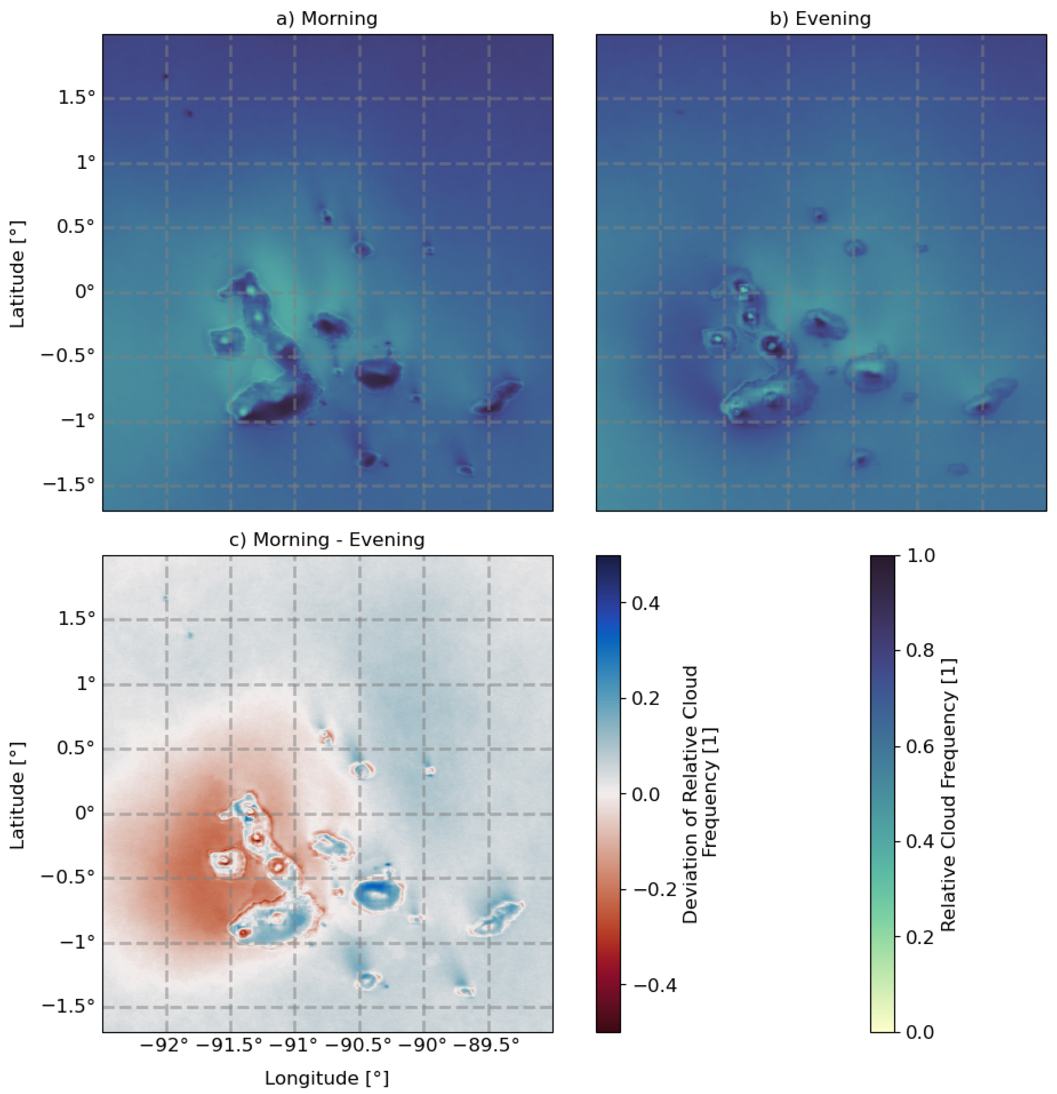
3.1. Spatial and Diurnal Distribution of Cloud Frequency

Figure 3 depicts the relative cloud frequency during morning and evening overpasses, as well as the difference between the two overpass times. In Figure 4a and Figure 5a, the cloud frequencies are presented as box plots of individual classes of the terrain elevation and aspect, respectively.

In general, the cloud frequency over the ocean is higher in the morning than in the evening. The area around Isabela is an exception, where the cloud cover is more pronounced in the evening than in the morning (Figure 3c). Moreover, the presence of clouds between the islands is less frequent than above the open ocean. During the morning, distinct “plumes” of higher cloud frequency occur north-west of some of the smaller islands (Figure 3a), which are not observed during the evening overpasses. Low values of relative cloud frequency are delineated on the coastal stripe of the islands, especially the western part of the archipelago, having an even lower frequency in the evening overpass.

Over the islands, the cloud frequency is generally higher in the morning, than in the evening. The mean cloud frequency of the land pixels is 0.71 in the morning, while it is 0.67 in the evening. However, not only the frequency, but also the spatial distribution of the clouds differs between the two times of day.

In the morning, a higher frequency of clouds is noticeable on the windward slopes facing the south and south-east of the islands at around >120°–210° (Figure 5a). The dependency on the terrain aspect is particularly prevalent for mid-altitudes, whereas it is equally low for the coastal region on all sides. Likewise, the summits of the volcanoes are characterized by a low cloud frequency, which is sharply separated from the higher cloud occurrences in the mid-altitudes. This is especially true for the volcanoes on the western part of the archipelago with altitudes above 900 $\mathrm{m}$ (Figure 3a,b and Figure 4a).

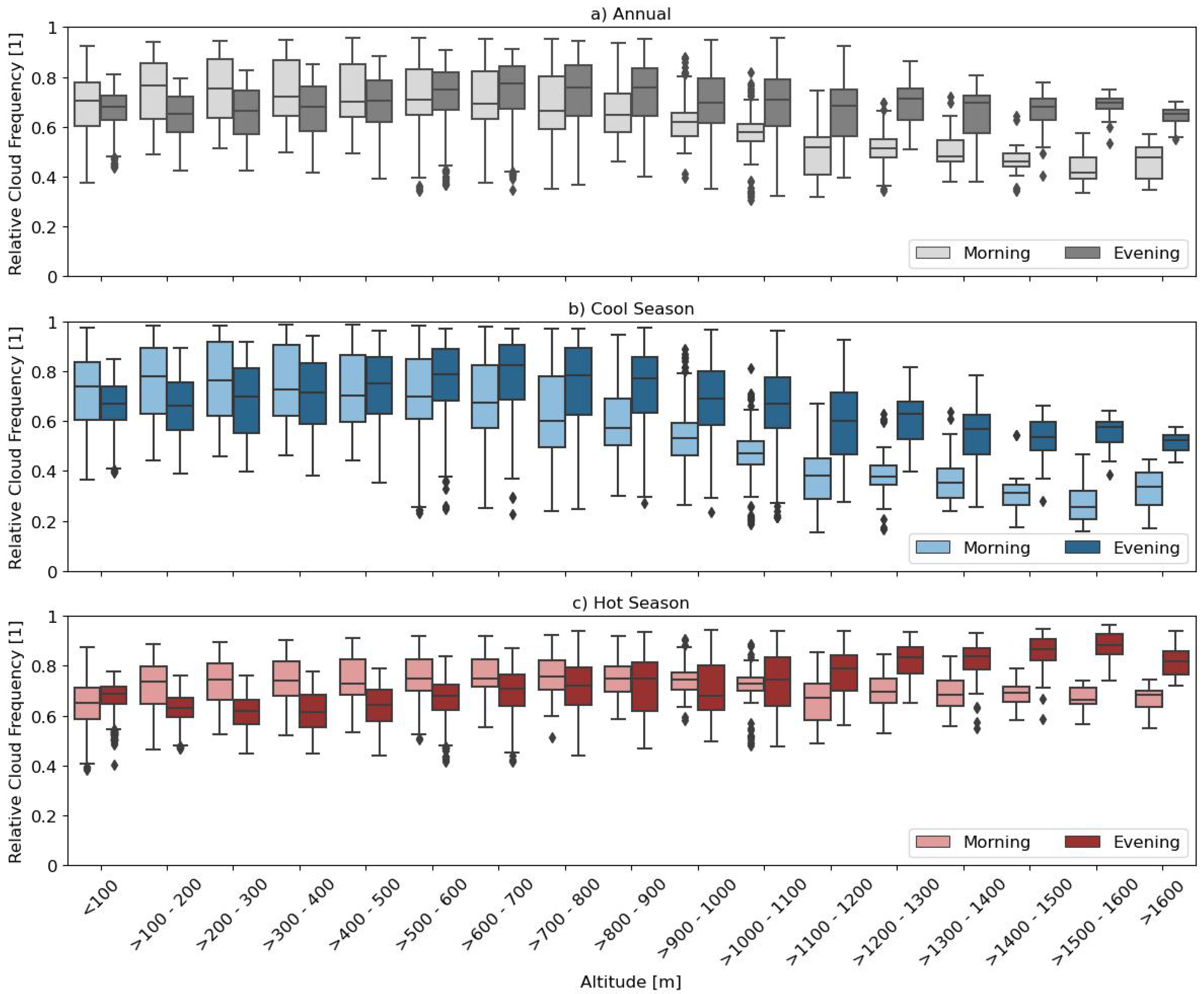
3.2. Seasonal Distribution of Cloud Frequency

Figure 6 shows the relative cloud frequency during the hot and cool seasons. It is visible that the spatial distribution of cloud coverage shows both diurnal and intra-annual variations.

Strongly attenuated differences between the windward and leeward sides of the islands characterize the hot season. The cloud frequency during the evening in the hot season shows a clear vertical zonation, and the influence of the aspect is almost absent (Figure 5c). Additionally, during the morning (Figure 6a), the differences between varied terrain heights (Figure 4c) are weakened and the clouds are relatively evenly distributed over the islands. During the evening, the cloud pattern shows a clear zonation along the altitude (Figure 6b). As depicted in Figure 4, coastal areas have a high cloud frequency, which decreases with increasing height until an elevation of ca. 400 $\mathrm{m}$. At this altitude, the cloud frequency starts to increase (Figure 4c). The highest cloud frequencies can be found at around 1500 $\mathrm{m}$–1600 $\mathrm{m}$, and only the summits higher than 1600 $\mathrm{m}$ have a lower frequency again. For the morning, the range of the medians of relative cloud frequency, depending on the altitude, ranges between 0.65 and 0.76. The difference between the highest and lowest median concerning the terrain aspect is just 0.08. The zonation is not as clearly visible as for the evening overpass (Figure 6a,c). Both times of day show almost no dependence on the aspect during the hot season. In the morning, very few clouds can be found over the sea, while, in the evening, an area of high cloud frequency appears west of Isabela.

During the cool season, spatial differences in cloud coverage are strongly pronounced. The difference between the uplands (volcanic peaks) and the highlands is particularly strong (Figure 6d,e). The medians of relative cloud frequency as a function of altitude range from 0.52 to 0.83 during the evening and belong to the classes >1600 $\mathrm{m}$ and >600$\mathrm{m}$–700$\mathrm{m}$, respectively (Figure 4c). The range of the median for the morning is shifted towards lower values. The altitude range >1500 $\mathrm{m}$–1600 $\mathrm{m}$ has the lowest median morning cloud frequency of 0.26, while the highest median of 0.78 is found at altitudes >100 $\mathrm{m}$–200 $\mathrm{m}$. In Figure 4b, the wide range of cloud frequency values for each altitude class reflects the big differences between the clear leeward side and the cloudy windward side of the islands. The difference between the highest and the lowest median depending on the terrain aspect, is 0.25 in the morning and 0.19 in the evening, which again illustrates that there is a greater windward–leeward gradient of cloud occurrence in the morning. Around Isabela, the cloud frequency over the sea is decreased, but most islands have plumes of higher cloud frequency in the north-east direction during the morning. Especially for the smaller islands, these plumes are strongly pronounced.

To compare the differences in cloud frequency, the data from the cool season were subtracted from the data from the hot season. The results are presented in Figure 6g,h for the morning and the evening, respectively. Positive values indicate a higher cloud frequency during the cool season, whereas negative values indicate the opposite.

For both times of day, the cloud coverage over the ocean is generally higher in the cool season than in the hot season. The evening overpasses show almost no seasonal variations in the area west of Isabela. On the islands, differences depend on the location, especially on the aspect and altitude, but also differ in strength on the individual islands of the archipelago (Figure 6). For both analyzed times of day, the south-east sides of the islands are more often covered by clouds in the cool season, whereas the north-west sides are cloudier during the hot season. The north of Isabela is an exception: the aspect seems to have hardly any influence on the cloud distribution. For the morning, this windward–leeward difference increases with rising altitude, as clearly seen at Santa Cruz and the southern part of Isabela. Here again, the northern region of Isabela is an exception, where, especially, the volcano Alcedo hardly shows any dependence on the aspect.

On the individual islands, the differences are pronounced to different degrees. The variances at Santa Cruz and San Cristóbal are more pronounced in the evening than in the morning, while, in the morning, differences are stronger on Isabela. The importance of the elevation and aspect varies, depending on the season, which is reflected in the results of the random forest regression (

Table 2. Results of the importance variable derivation based on the random forest regression.

	Hot Season		Cool Season
	Morning	Evening	Morning	Evening
Altitude	0.57	0.63	0.56	0.40
Aspect	0.43	0.37	0.44	0.60

). In the hot season, cloud frequency depends more on altitude, while, in the cool season, the influence of the aspect plays a greater role. In both seasons, the values are further apart in the evening and closer together in the morning.

3.3. Cloud Frequency Analysis in Extreme Events

Figure 7 depicts the deviation in the relative cloud frequency of the ENSO events El Niño 2015 and La Niña 2007 corresponding to the “normal” relative cloud frequency of the comparison period (Section 2.7) for both times of day.

Figure 7a illustrates that the median relative cloud frequency was higher in both the evening and morning during El Niño 2015 than during a typical period from May to January. This increased cloud frequency is quantified by the increase in the median by 0.06 in the morning and 0.04 in the evening. In addition to the median, the entire range of cloud frequency values also increases during the extreme event, although the range of values remains approximately the same. Since only land pixels were considered in this analysis, a general increase in cloud occurrence over the islands during El Niño 2015 can be observed. The opposite can be observed for La Niña 2007. As shown in Figure 8b, the medians of the relative cloud frequency during the La Niña event in 2007 were lower than in the “normal” comparison period. The decrease was −0.05 in the morning and −0.02 in the evening. Furthermore, the interquartile range and the general range of values of relative cloud frequency were larger than normal. This indicates that there were fewer clouds during La Niña 2007, but, at the same time, the differences in the spatial distribution of clouds were more pronounced. All four samples (El Niño morning/evening, La Niña morning/evening) revealed a statistically significant deviation from their respective comparative data sets, with p-values less than 0.05.

The spatial variations of the deviation in the cloud frequency during El Niño 2015 and La Niña 2007 are presented in Figure 7. During El Niño 2015, the relative cloud frequency over the islands was mostly higher than normal (Figure 7a,b). The increases in the morning were mainly located at the north-western slopes, whereas hardly any changes could be seen on the windward (south-east facing) slopes. The biggest increase in cloud occurrence was observed over the leeward slopes of Isabela and Fernandina. The maximum deviation with the value 0.352 was found on the summit of Cerro Azul, the south-east summit of Isabela. In the evening, the deviation showed a more fragmented pattern. The cloud frequency over the leeward slopes mostly increased. The leeward slopes showed an increase in the lower areas, but a decrease in the higher elevations, as exemplified for Santa Cruz. The deviation over the sea area showed spatial differences. During the evening, more areas revealed an increase, whereas, in the morning, most of the sea pixels showed a decrease in cloud frequency. For both times of day, the area around Isabela recorded an increase in cloud occurrence, whereas the south-eastern part of the study area recorded an increase.

It is apparent from Figure 7c,d, that the cloud frequency during La Niña 2007 was lower than usual over the islands, but higher over the ocean, with an exception of the area between Isabela and Fernandina. Strong decreases occurred mainly on the islands’ leeward sides (north-west) and at high altitudes. The strongest reduction was observed on the Sierra Negra volcano on Isabela, with a decline of −0.313 in the morning and −0.185 in the evening. For the evening, again, a more complex pattern was recorded. The summits again showed the strongest decrease. However, clear dependence on the aspect was recognizable. Most of the leeward slopes showed decreases, while those at the north of Isabela showed larger decreases.

4. Discussion

4.1. Spatial and Diurnal Variations in Cloud Frequency

The climate of tropical landmasses is dominated by a diurnal cycle [38], which is also reflected in the cloud frequency over the Galapagos archipelago. The spatio-temporal patterns of relative cloud frequency are the result of the interplay between large-scale (macroscale) circulation and mesoscale thermally induced wind systems leading to cloud formation.

The synoptic trade winds can be identified as one of the main drivers of the macroscale pattern of cloud distribution on the Galapagos Islands. The cloud frequency on the windward sides of the archipelago is much higher than on the leeward sides, especially on the islands with higher elevations, that are not in the lee of other islands (Isabela, Santa Cruz, San Cristóbal). The south-easterly trade winds, combined with orographic lifting, lead to cloud development on windward slopes [18]. This is in line with observations made on different tropical islands such as the Island of Hawai’i [18] and Nauru [39], which also underlie the influence of prevailing trade winds and record higher cloud occurrence on the windward island sides. The observed cloud frequency differences between windward and leeward slopes are smaller in the evening than in the morning (Figure 6). These diurnal variations were also described, e.g., for the Island of Hawai’i [18] and are a result of the strengthened winds during the day over the island. Due to the diurnal heating of the islands, vertical mixing is induced, and winds are strengthened during the day [18], while, at night, when the atmospheric conditions are stable, the surface winds are reduced [18]. This results in increased cloud development during the day over windward slopes [18]. It can be assumed that, at terrestrial Galapagos, a similar effect leads to these diurnal differences, even if area-wide local surface wind data are missing, to confirm this assumption completely. Regions of moderate altitude (approximately 100 $\mathrm{m}$–900 $\mathrm{m}$) show the highest cloud frequency (Section 3.2), both in the evening and the morning.

The volcanic summits have a low cloud frequency. This phenomenon only occurs on those summits of the archipelago that reach into the trade-inversion layer, which occurs in the hot season month at a height of approx. 900 $\mathrm{m}$–1100 $\mathrm{m}$ (Figure S7). Since the inversion layer prevents the vertical expansion of the clouds, the peaks remain cloud-free. Similar observations have been made on the Island of Hawai’i, where the altitude of the summits of Mts. Loa and Kea exceed the local height of the trade wind inversion, and, therefore, are characterized by low cloud occurrence [40].

These macroscale effects can be modified by local-scale effects, resulting in deviations from the larger-scale cloud patterns. One of the drivers for local scale effect is the diurnal heating of the land, leading to thermally driven flows. Due to the lower heat capacity of the land, the land surface heats up faster than the sea surface [41]. This leads to a temperature gradient and, thus, to a pressure gradient between the land and sea surface. When the humidity of the air is high enough, cloud forming over the land is induced [41]. Thermal convection also causes upslope winds on mountainsides [42], which can amplify the existing sea breeze [41]. The higher cloud frequencies at all sides of the islands, observed at the lower elevations (up to around 600 $\mathrm{m}$) during daytime (morning overpass), stands in line with this theoretical description (Figure 3c).

During the night, the difference between temperature and air pressure inverts and the land breeze forms [41]; hence, the clouds form over the sea. If there is no additional forcing, the sea breeze should be the same on all sides of the islands [41] and lead to an evenly distributed cloud pattern on all coastlines. A slope facing the seaside can amplify the sea breeze due to the temperature cycle of the hill surface [41] Additionally, katabatic flows develop during night, when the land surfaces cools and the pressure gradient and the buoyancy reverse compared to the day, leading to a downslope wind [43]. In combination with the nocturnal land breeze, this explains the higher cloud formation over the coastal waters during night (evening overpass) compared to the day (morning overpass), which is observed along all the sides of the islands (Figure 3c).

Another thermodynamic driver of cloud formation is local SST fields. Comparing the cloud frequency distribution over the sea (Figure 3) with averaged maps of SST (Figure S8). illustrates the strong influence of the SST pattern. Particularly noticeable is the sea area west of Isabela, which is characterized by a lower SST, due to the cold upwelling of the equatorial undercurrent. During the evening, when the deviation of SST in this area is stronger, a higher cloud frequency is observed. The cooler SST leads to the formation of low clouds [44] and explains the higher cloud occurrences in this area, compared to the low cloud frequency area west of Isabela.

Leeward from the islands, plumes of higher cloud frequency are observed. During the evening, only weak plumes north-west of the bigger islands (Santiago, Santa Cruz, and Isabela) occur, whereas, in the morning, the smaller islands also display particularly strong plumes. Cloud plumes are a phenomenon well-described in the literature since they were observed on multiple islands such as Nauru [39] and the Island of Hawai’i [40,45]. All these studies have in common that the cloud bands have the highest intensity in the afternoon. Different mechanisms cause cloud plumes, depending on the size and topography of the island, as well as on the wind speed [46]. For smaller islands with low maximum altitudes, such as Nauru (max. height 60 $\mathrm{m}$), the plume formation is based on the diurnal heating of the land combined with the advection of moist air to the island by prevailing trade winds [39,47]. The so-induced clouds are then advected downwind, resulting in a cloud plume leeward of the island [39,47]. Since the cloud plumes found at Galapagos are not continuous from the inland of the islands to the sea, but are instead disrupted by a lower cloud frequency area over the coast (Figure 6d), another mechanism must cause this cloud plume formation. A second mechanism is described for taller islands, where the mountain elevation exceeds the height of the trade inversion e.g., Hawai’i and, thus, represents a technical obstacle to the airflow [45,46]. Due to the inversion layer, the flow is forced to surround the obstacle [43]. When rejoining in the lee of the island, the confluence of the flow induces convection and leads to cloud formation, thereby forming a plume [43,45]. This hypothesis is in line with the observed plume patterns starting behind the islands. Reasons for the strong plumes in the morning are due to the strong inversion layer resulting from nocturnal cooling, which leads to a surround flow and, thus, the lee confluence must be strongest, leading to particularly strong cloud plumes at smaller islands in the archipelago such as Pinta, Marchena, Floreana, and Española. Conversely, in the evening, the inversion layer weakens, and, therefore, weak plumes are only apparent on the bigger islands of Santiago, Santa Cruz, and Isabela.

4.2. Seasonal Differences

The interaction of thermal and mechanical forcing produces rich seasonal patterns of cloud frequency [48], which were also observed on the Galapagos archipelago (Section 3.2). During the hot season, the trade winds are weakened and the SST is increased (e.g., [15]). This weakens the influence of mechanical forcing, and thermal convection becomes the main driver of cloud formation. This is reflected in a relatively homogeneous cloud cover over all sides of the island (Figure 6). The random forest regression underlines this finding, by resulting in a higher value of importance for the altitude than the aspect for both overpass times (Table 2) (more detailed results can be found in Figures S9 and S10). In the absence of mechanical forcing, the effect of the land–sea breeze is evenly distributed over the coastal regions of all orientations of the islands and clearly visible for the evening overpasses in Figure 6a. The cloudy area west of Isabela is characterized by a lower SST caused by the Pacific equatorial undercurrent (Figure S8), leading to the formation of low stratus clouds [44]. During the day, the SST increases, leading to suppression of low cloud formation, especially during the hot season. A slight decrease in cloud frequency at the summits of the volcanoes is probably caused by the occasional occurrence of the inversion layer, at the beginning and end of the hot season (map of the mean base height of the trade wind inversion layer can be found in Figure S7). Generally, the decrease in very low altitudes is slight and, in mid-elevations, the cloud frequency increases first with elevation and then slightly decreases. This mainly corresponds to the observed rainfall patterns in the hot season, which describe dry lowlands and increasing orographic rainfall with increasing altitude [1,12,25]. Cloud plumes over the ocean are almost non-existent, which is consistent with the decrease in the trade winds, as they were identified as a driver of the forming process. Additionally, on Nauru, the plume occurs significantly more scarcely during the period in which the local prevailing easterly trade winds are declined [39].

In reverse, when the trade winds are strong during the cool season, the mechanical forcing dominates the convection. This causes strong differences between windward and leeward sides, as seen in Figure 6b. In combination with a low SST, the trade wind also leads to a strong formation of the trade wind inversion (e.g., [12]). This explains the strong decrease in cloud frequency above an altitude of approximately 900 $\mathrm{m}$ (Figure 6). The dominance of the mechanical forcing leads to a higher importance of the aspect than the altitude to explain the cloud frequency distribution (Table 2). When the air, transported by the trade winds, hits the islands, it is forced to rise [12,14]. The orographic lifting leads to the formation of Garúa [12,14] and explains the higher cloud occurrence on the windward sides. The strong prevailing wind also leads to the formation of cloud plumes, as explained above.

The high cloud frequency over the ocean during the cool season is related to the lowered SST and the associated increased formation of low stratus clouds [44]. In the area of the undercurrent, a higher cloud frequency is visible during the evening. This is again caused by the higher temperature gradient between the sea surface temperature of this area and the surrounding areas.

4.3. Extreme Events

The detected increase in cloud frequency during the warm event El Niño 2015 is an expression of the higher convective activity due to increased SST [49]; not only the coastal region, but all altitudes are affected. Higher SST also weakens the inversion layer because the lower air layers are not cooled as much while passing over the ocean. This explains the particularly strong rise in cloud coverage in the uplands. The increased in cloud frequency, especially on the leeward sides (Section 3.3), is due to the weakened trade winds, which are observed during warm events at Galapagos [14,24] and strengthened thermal convection. Although the cloud frequency increased during El Niño 2015, there was no augmented rainfall in 2015/16 [24], as is usually the case in the Galapagos Islands during El Niño events [50]. Therefore, it would be interesting to compare the cloud occurrence with other El Niño events to see if there were any unusual cloud patterns during El Niño 2015. Tye and Aldáz [50] observed that, during the El Niño event in 1997–1998, Garúa did not develop. During El Niño 2015, the cloud frequency was relatively evenly distributed over the islands, which would again support the hypothesis that the convective activity was increased and the trade winds were weakened, leading to decreased advection, resulting in the suppression of Garúa formation.

During La Niña 2007, the Pacific stratus was intensified, but not the low stratus over the islands. The leeward sides of the island showed a strong decrease in cloud frequency, whereas, on the windward sides, the cloud frequency only decreased slightly (Section 3.3). The increased trade winds can explain the strengthened lee-effect during the cold event [24]. The exceptionally cold SST during La Niña events [14] cools the lower air layers even more than usual and, thus, reinforces the inversion layer, which causes the particularly low cloud frequency in the uplands. At the same time, the cold SST increases the formation of low stratus clouds over the Pacific [44], which is reflected in the unusually high cloud frequency that was found over the ocean. Surprisingly, the windward sides of the islands did not show an increased cloud frequency. This could be due to the solar heating of the island, which clears the stratus clouds. Snell and Rea [25] found that, in La Niña years, there was very low rainfall at Galapagos, which stands in line with our detection of lower cloud frequencies.

4.4. Uncertainties in Data and Method

The MODIS cloud mask is based on two different retrieval paths that distinguish between daytime and nighttime data. The paths differ in the threshold tests applied and the adjusted thresholds for cloud detection. A comparison with Cloud-Aerosol Lidar with Orthogonal Polarization (CALIOP) cloud detection showed that the cloud detection rate for both land and water pixels was lower at nighttime (evening) than during the daytime (morning). For the geographic region 60° N to 60° S, the differences between the detection rates do not exceed 1.6% [51]. Since the differences in the cloud frequency found between the morning and evening overpasses were mostly larger than this retrieval-based deviation, it can be concluded that they are caused by diurnal heating and changing of the wind patterns during the course of the day.

Additionally, the resampling of the terrain data is accompanied by a loss of accuracy. Especially in regions with steep slopes, such as volcano craters, the spatial resolution of 1 km leads to the smoothing of terrain features and potential loss of details. Statistics on the mean deviations of the 30 mpixel height in each 1 pixel can be found in Figure S11. The highest mean of deviations occurs in the height class >1600 $\mathrm{m}$, where the average deviation from the 1 pixels to the 30 $\mathrm{m}$ pixels is $-60$ $\mathrm{m}$.

Further uncertainties are induced by basing the analysis on monthly averages. It should be noted that the monthly averages can be based on different numbers of satellite images, e.g., due to different lengths of months and missing satellite scenes. Thus, the weighting of the individual values to the overall relative cloud frequency was not identical for all days. In order to estimate the resulting error, the following calculation was carried out: $\sum \left(\frac{\# \mathrm{available} \mathrm{days} \mathrm{per} \mathrm{month}}{\# \mathrm{days} \mathrm{per} \mathrm{month}}\right)/12$. With this approach, the induced error over the entire period can be quantified as <4.5% (equals a deviation of cloud frequency <0.045), which is lower than most of the observed differences in the cloud pattern.

5. Conclusions

In this study, the cloud frequency of the Galapagos archipelago was analyzed by evaluating 21 years of MODIS cloud mask data, over the time period from 25 February 2000 to 31 December 2021. Two overflights per day were analzsed, originating from the morning (between 9:20 and 11:45 local time) and from the evening (21:20 and 23:40 local time). The data were evaluated concerning spatio-temporal patterns, as well as differences that were caused by ENSO events. The main findings of this study are as follows:

• The cloud frequency reaches its maximum in the highlands, while it decreases abruptly in the uplands, due to the inversion layer;
• The windward, south-eastern slopes are more often covered by clouds than the leeward, north-western slopes. This is caused by the south-eastern trade winds;
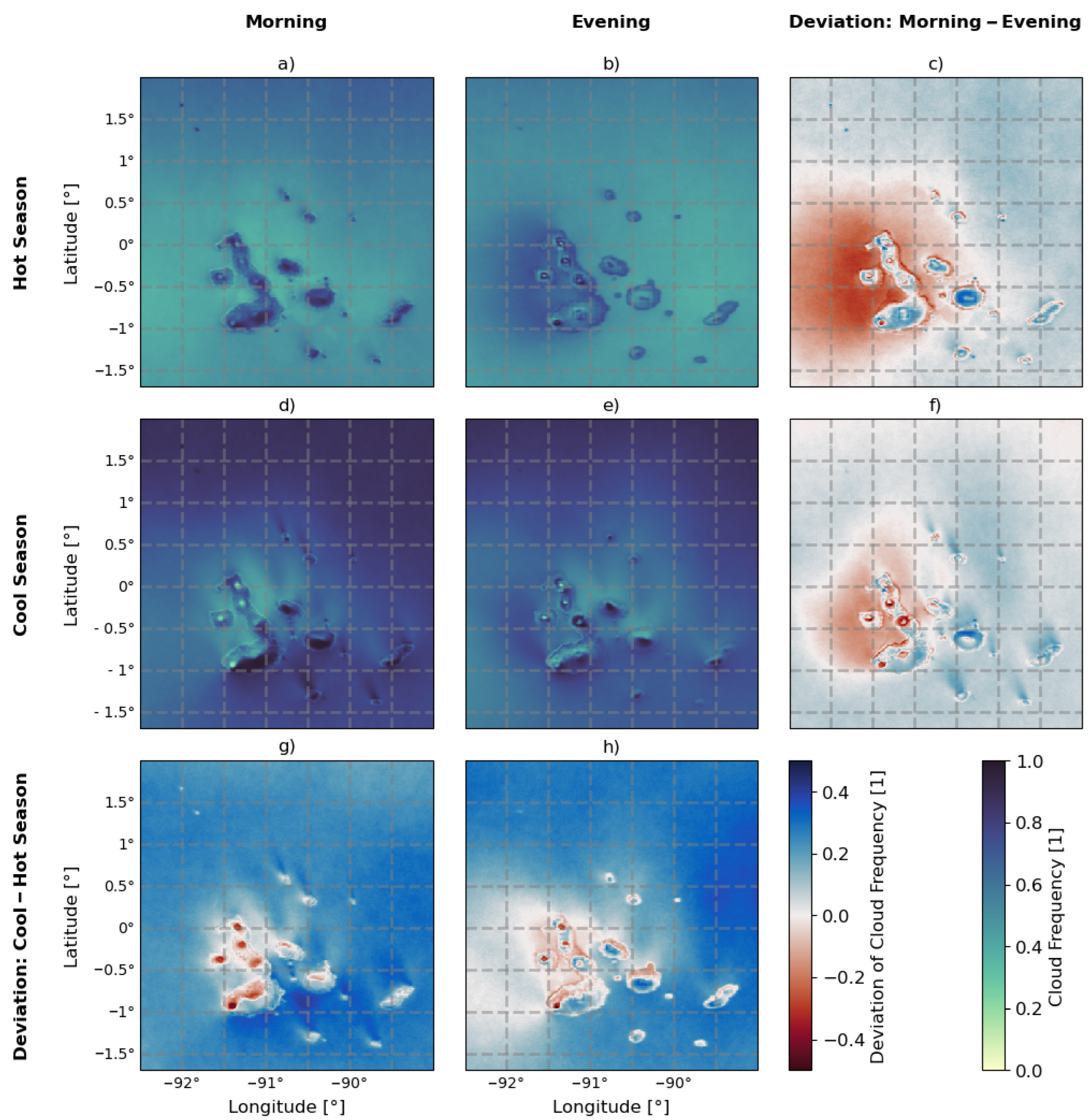
• Diurnal differences in cloud frequency vary spatially, but the general cloud frequency over the islands is lower in the evening than in the morning;
• During the hot season, the cloud frequency over the islands is higher and more evenly distributed than during the cool season, both in the evening and the morning;
• The distribution of cloud frequency is more dependent on terrain altitude than on aspect during the hot season, while the opposite is true during the cool season;
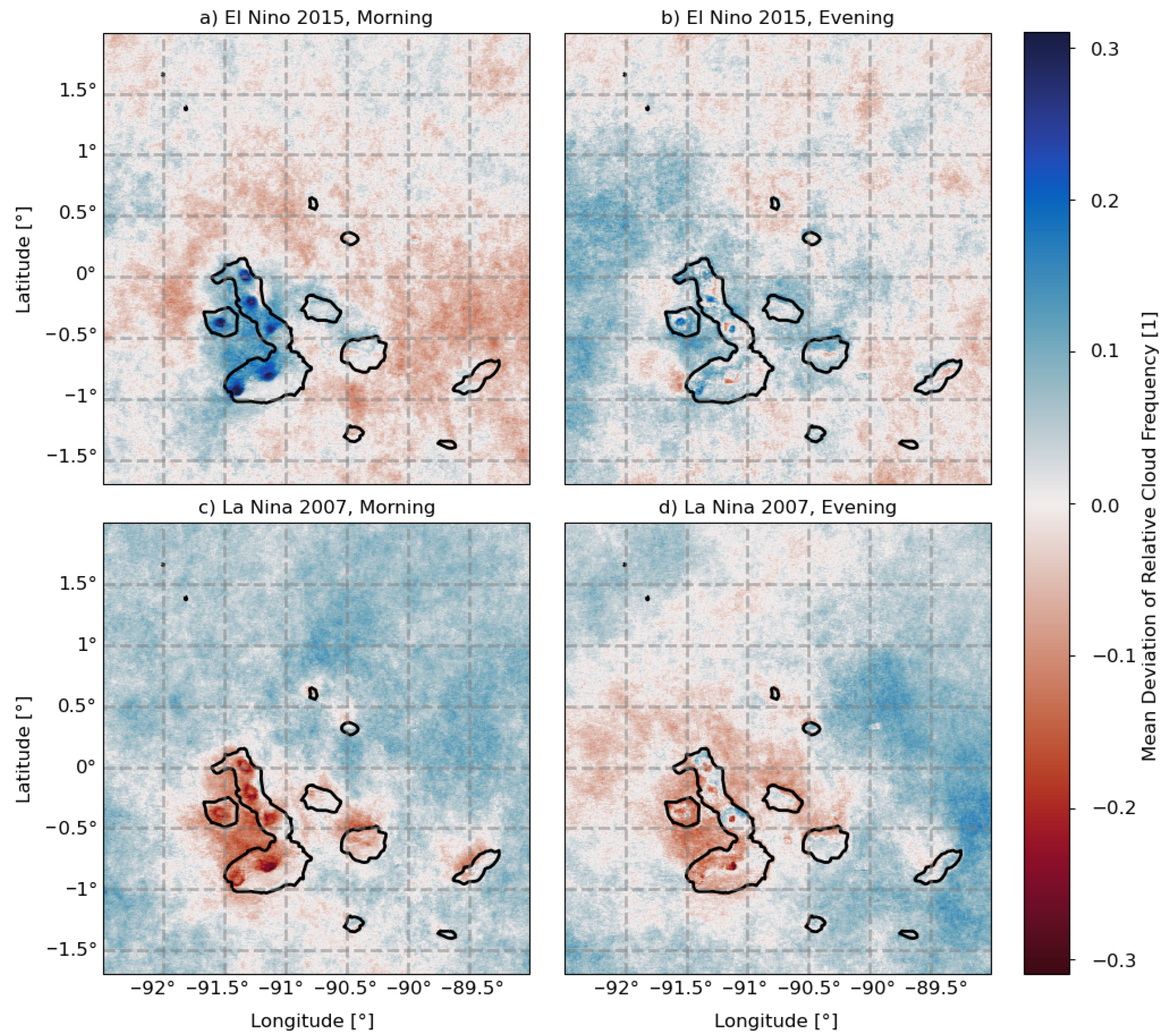
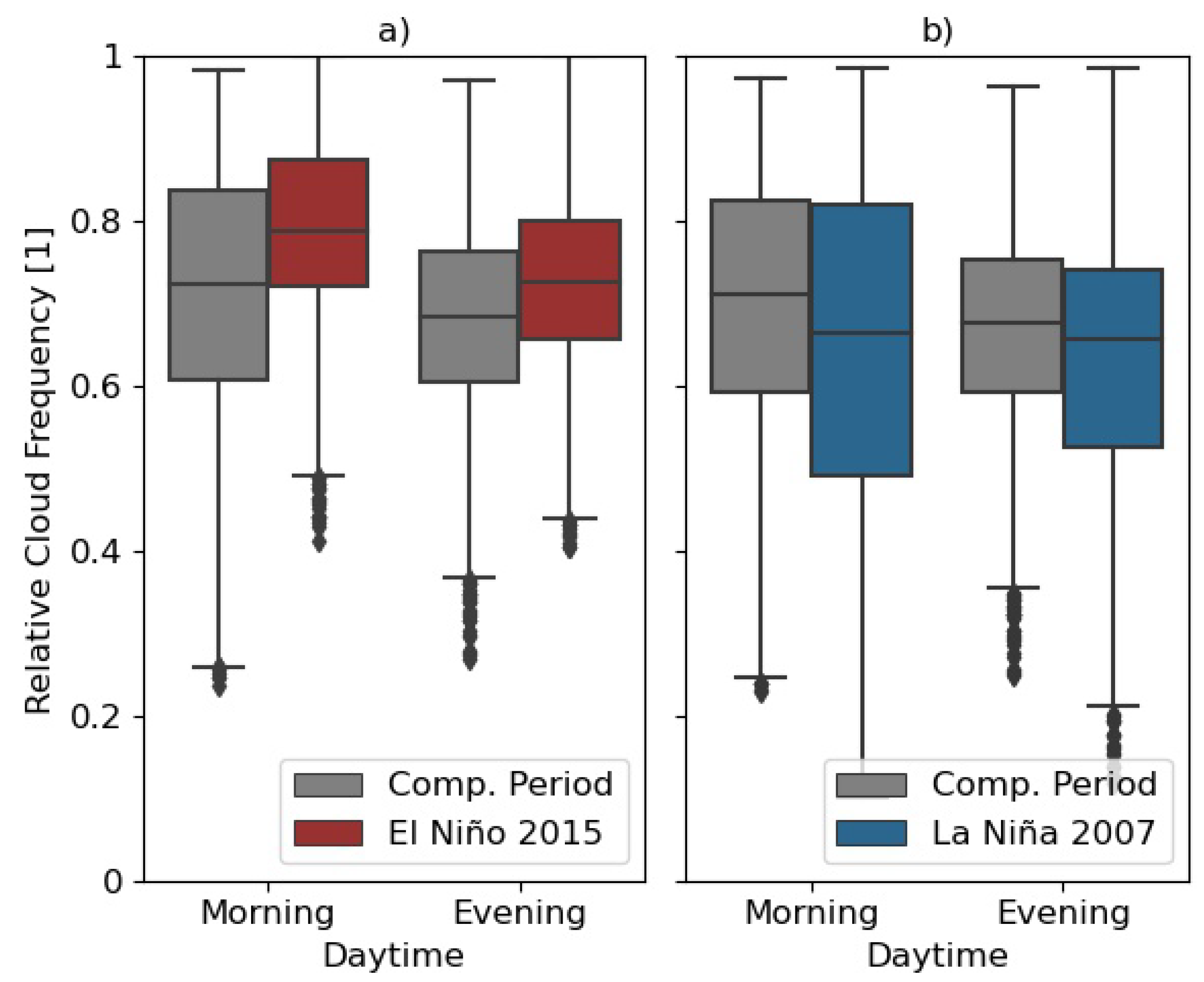
• During El Niño 2015, the leeward sides, as well as the uplands, showed an increase in cloud coverage. Therefore, spatial differences in cloud frequency were less pronounced;
• La Niña 2007 had the opposite effect of El Niño 2015. The cloud frequency of the leeward sides and the upland areas showed a decreased cloud frequency. The cloud frequency over the ocean increased.

In future studies, breaking down the detected clouds according to their types would be useful. This would give more information about the formation mechanisms and possible changes in the frequency of occurrence of individual cloud types over the observation period. Additionally, analyzing data from a more extended observation period would help further investigate trends. For example, the cloud mask of the Advanced Very High Resolution Radiometer (AVHRR) could be used. This would provide data from 1978 onwards, but the spatial resolution would be reduced to 4 $\mathrm{k}$$\mathrm{m}$ at the nadir [52]. This long time series would allow multiple strong ENSO events to be compared.

References

- Escobar-Camacho, D.; Rosero, P.; Castrejón, M.; Mena, C.F.; Cuesta, F. Oceanic islands and climate: Using a multi-criteria model of drivers of change to select key conservation areas in Galapagos. Reg. Environ. Chang. 2021, 21, 47. [Google Scholar] [CrossRef]
- Hobday, A.J.; Pecl, G.T. Identification of global marine hotspots: Sentinels for change and vanguards for adaptation action. Rev. Fish Biol. Fish. 2014, 24, 415–425. [Google Scholar] [CrossRef]
- Paltán, H.A.; Benitez, F.L.; Rosero, P.; Escobar-Camacho, D.; Cuesta, F.; Mena, C.F. Climate and sea surface trends in the Galapagos Islands. Sci. Rep. 2021, 11, 14465. [Google Scholar] [CrossRef]
- Dueñas, A.; Jiménez-Uzcátegui, G.; Bosker, T. The effects of climate change on wildlife biodiversity of the galapagos islands. Clim. Change Ecol. 2021, 2, 100026. [Google Scholar] [CrossRef]
- IPCC. Contribution of Working Group I to the Sixth Assessment Report of the Intergovernmental Panel on Climate Change; Cambridge University Press: Cambridge, UK, 2021.
- An, N.; Wang, K.; Zhou, C.; Pinker, R.T. Observed variability of cloud frequency and cloud-base height within 3600 m above the surface over the contiguous United States. J. Clim. 2017, 30, 3725–3742. [Google Scholar] [CrossRef]
- Ramanathan, V.; Cess, R.D.; Harrison, E.F.; Minnis, P.; Barkstrom, B.R.; Ahmad, E.; Hartmann, D. Cloud-Radiative Forcing and Climate: Results from the Earth Radiation Budget Experiment. Science 1989, 243, 57–63. [Google Scholar] [CrossRef]
- Stocker, T.F.; Qin, D.; Plattner, G.K.; Alexander, L.V.; Allen, S.K.; Bindoff, N.L.; Bréon, F.M.; Church, J.A.; Cubasch, U.; Emori, S.; et al. Climate change 2013: The physical science basis. Contribution of Working Group I to the Fifth Assessment Report of the Intergovernmental Panel on Climate Change, Technical summary; Cambridge University Press: Cambridge, UK, 2013; pp. 33–115. [Google Scholar]
- Quante, M. The role of clouds in the climate system. J. Phys. IV Proc. 2004, 121, 61–86. [Google Scholar] [CrossRef]
- Bony, S.; Stevens, B.; Frierson, D.M.; Jakob, C.; Kageyama, M.; Pincus, R.; Shepherd, T.G.; Sherwood, S.C.; Siebesma, A.P.; Sobel, A.H.; et al. Clouds, circulation and climate sensitivity. Nat. Geosci. 2015, 8, 261–268. [Google Scholar] [CrossRef]
- Stephens, G.L. Cloud Feedbacks in the Climate System: A Critical Review. J. Clim. 2005, 18, 237–273. [Google Scholar] [CrossRef]
- Trueman, M.; d’Ozouville, N. Characterizing the Galápagos terrestrial climate in the face of global climate change. Galapagos Res. 2010, 67, 26–37. [Google Scholar]
- Domínguez, C.G.; Vera, M.F.G.; Chaumont, C.; Tournebize, J.; Villacís, M.; d’Ozouville, N.; Violette, S. Quantification of cloud water interception in the canopy vegetation from fog gauge measurements. Hydrol. Process. 2017, 31, 3191–3205. [Google Scholar] [CrossRef]
- Sachs, J.P.; Ladd, S.N. Climate and oceanography of the Galapagos in the 21st century: Expected changes and research needs. Galapagos Res. 2010, 67, 50–54. [Google Scholar]
- Echeverría, P.; Domínguez, C.; Villacís, M.; Violette, S. Fog harvesting potential for domestic rural use and irrigation in San Cristobal Island, Galapagos, Ecuador. Geogr. Res. Lett. 2020, 46, 563–580. [Google Scholar] [CrossRef]
- Pryet, A.; Dominguez, C.; Tomai, P.F.; Chaumont, C.; d’Ozouville, N.; Villacís, M.; Violette, S. Quantification of cloud water interception along the windward slope of Santa Cruz Island, Galapagos (Ecuador). Agric. For. Meteorol. 2012, 161, 94–106. [Google Scholar] [CrossRef]
- Halladay, K.; Malhi, Y.; New, M. Cloud frequency climatology at the Andes/Amazon transition: 1. Seasonal and diurnal cycles. J. Geophys. Res. Atmos. 2012, 117. [Google Scholar] [CrossRef]
- Barnes, M.L.; Miura, T.; Giambelluca, T.W. An Assessment of Diurnal and Seasonal Cloud Cover Changes over the Hawaiian Islands Using Terra and Aqua MODIS*. J. Clim. 2016, 29, 77–90. [Google Scholar] [CrossRef]
- Bendix, J.; Rollenbeck, R.; Göttlicher, D.; Cermak, J. Cloud occurrence and cloud properties in Ecuador. Clim. Res. 2006, 30, 133–147. [Google Scholar] [CrossRef]
- Alpert, L. Notes on the weather and climate of Seymour Island, Galapagos Archipelago. Bull. Am. Meteorol. Soc. 1946, 27, 200–209. [Google Scholar] [CrossRef][Green Version]
- Colinvaux, P.A. Climate and the Galapagos Islands. Nature 1972, 240, 17–20. [Google Scholar] [CrossRef]
- Atwood, A.R.; Sachs, J.P. Separating ITCZ- and ENSO-related rainfall changes in the Galápagos over the last 3 kyr using D/H ratios of multiple lipid biomarkers. Earth Planet. Sci. Lett. 2014, 404, 408–419. [Google Scholar] [CrossRef]
- Glantz, M.H.; Ramirez, I.J. Reviewing the Oceanic Niño Index (ONI) to Enhance Societal Readiness for El Niño’s Impacts. Int. J. Disaster Risk Sci. 2020, 11, 394–403. [Google Scholar] [CrossRef]
- Martin, N.J.; Conroy, J.L.; Noone, D.; Cobb, K.M.; Konecky, B.L.; Rea, S. Seasonal and ENSO Influences on the Stable Isotopic Composition of Galápagos Precipitation. J. Geophys. Res. Atmos. 2018, 123, 261–275. [Google Scholar] [CrossRef]
- Snell, H.; Rea, S. The 1997-98 El Niño in Galápagos: Can 34 years of data estimate 120 years of pattern? Not. Galápagos 1999, 60, 111–120. [Google Scholar]
- Platnick, S.; Ackerman, S.; King, M.; Meyer, K.; Menzel, W.; Holz, R.; Baum, B.; Yang, P. MODIS Atmosphere L2 Cloud Mask Product (35_L2), NASA MODIS Adaptive Processing System; Goddard Space Flight Center: Glenn Dale, MD, USA, 2015. [CrossRef]
- Frey, R.A.; Ackerman, S.A.; Liu, Y.; Strabala, K.I.; Zhang, H.; Key, J.R.; Wang, X. Cloud Detection with MODIS. Part I: Improvements in the MODIS Cloud Mask for Collection 5. J. Atmos. Ocean. Technol. 2008, 25, 1057–1072. [Google Scholar] [CrossRef]
- Team MODIS Cloud Mask; Ackerman, S.; Strabala, K.; Menzel, P.; Frey, R.; Moeller, C.; Gumley, L.; Baum, B.; Schaaf, C.; Riggs, G. Discriminating Clear-Sky from Cloud with Modis Algorithm Theoretical Basis Document (mod35). 2010. Available online: https://atmosphere-imager.gsfc.nasa.gov/sites/default/files/ModAtmo/MOD35_ATBD_Collection6_1.pdf (accessed on 15 May 2023).
- NASA/METI/AIST/Japan Space Systems and U.S./Japan ASTER Science Team. ASTER global digital elevation model [data set]. NASA EOSDIS Land Processes Distributed Active Archive Center, 2009. Available online: https://doi.org/10.5067/ASTER/ASTGTM.002 (accessed on 21 March 2022).
- HEG-C (HDF-EOS to GeoTIFF Converter). v2.14. Greenbelt, MD: Earth Science Data and Information System (ESDIS) Project, Earth Science Projects Division (ESPD), Flight Projects Directorate, Goddard Space Flight Center (GSFC) National Aeronautics and Space Administration (NASA). 2017. Available online: https://wiki.earthdata.nasa.gov/display/DAS/Downloads (accessed on 20 November 2021).
- Strabala, K.I. MODIS Cloud Mask User’s Guide; University of Wisconsin–Madison: Madison, WI, USA, 2005. Available online: https://atmosphere-imager.gsfc.nasa.gov/sites/default/files/ModAtmo/CMUSERSGUIDE_0.pdf (accessed on 17 May 2023).
- Breiman, L. Random forests. Mach. Learn. 2001, 45, 5–32. [Google Scholar] [CrossRef]
- Pedregosa, F.; Varoquaux, G.; Gramfort, A.; Michel, V.; Thirion, B.; Grisel, O.; Blondel, M.; Prettenhofer, P.; Weiss, R.; Dubourg, V.; et al. Scikit-learn: Machine Learning in Python. J. Mach. Learn. Res. 2011, 12, 2825–2830. [Google Scholar]
- Breiman, L.; Friedman, J.H.; Olshen, R.A.; Stone, C.J. Classification and Regression Trees; Wadsworth Int. Group: Belmont, CA, USA, 1984. [Google Scholar]
- NOAA (National Oceanic and Atmospheric Administration). Cold and Warm Episodes by Season. 2022. Available online: https://origin.cpc.ncep.noaa.gov/products/analysis_monitoring/ensostuff/ONI_v5.php (accessed on 30 April 2022).
- Conroy, J.L.; Overpeck, J.T.; Cole, J.E.; Shanahan, T.M.; Steinitz-Kannan, M. Holocene changes in eastern tropical Pacific climate inferred from a Galápagos lake sediment record. Quat. Sci. Rev. 2008, 27, 1166–1180. [Google Scholar] [CrossRef]
- Mann, H.B.; Whitney, D.R. On a test of whether one of two random variables is stochastically larger than the other. Ann. Math. Stat. 1947, 18, 50–60. [Google Scholar] [CrossRef]
- Hendon, H.H.; Woodberry, K. The diurnal cycle of tropical convection. J. Geophys. Res. 1993, 98, 16623. [Google Scholar] [CrossRef]
- McFarlane, S.A.; Long, C.N.; Flynn, D.M. Impact of Island-Induced Clouds on Surface Measurements: Analysis of the ARM Nauru Island Effect Study Data. J. Appl. Meteorol. 2005, 44, 1045–1065. [Google Scholar] [CrossRef]
- Yang, Y.; Xie, S.P.; Hafner, J. Cloud patterns lee of Hawaii Island: A synthesis of satellite observations and numerical simulation. J. Geophys. Res. 2008, 113, D15126. [Google Scholar] [CrossRef]
- Miller, S.T.; Keim, B.D.; Talbot, R.W.; Mao, H. Sea breeze: Structure, forecasting, and impacts. Rev. Geophys. 2003, 41, 1–31. [Google Scholar] [CrossRef]
- Wang, C.C. Thermally-Driven Circulation and Convection over a Mountainous Tropical Island. Master’s Thesis, Department of Atmospheric and Oceanic Sciences, McGill University, Montreal, QC, Canada, 2014. [Google Scholar]
- Kirshbaum, D.; Adler, B.; Kalthoff, N.; Barthlott, C.; Serafin, S. Moist Orographic Convection: Physical Mechanisms and Links to Surface-Exchange Processes. Atmosphere 2018, 9, 80. [Google Scholar] [CrossRef]
- Luo, J.J.; Wang, G.; Dommenget, D. May common model biases reduce CMIP5’s ability to simulate the recent Pacific La Niña-like cooling? Clim. Dyn. 2018, 50, 1335–1351. [Google Scholar] [CrossRef]
- Smith, R.B.; Grubišić, V. Aerial Observations of Hawaii’s Wake. J. Atmos. Sci. 1993, 50, 3728–3750. [Google Scholar] [CrossRef]
- Matthews, S.; Hacker, J.M.; Cole, J.; Hare, J.; Long, C.N.; Reynolds, R.M. Modification of the Atmospheric Boundary Layer by a Small Island: Observations from Nauru. Mon. Weather. Rev. 2007, 135, 891–905. [Google Scholar] [CrossRef][Green Version]
- Nordeen, M.L.; Minnis, P.; Doelling, D.R.; Pethick, D.; Nguyen, L. Satellite observations of cloud plumes generated by Nauru. Geophys. Res. Lett. 2001, 28, 631–634. [Google Scholar] [CrossRef]
- Wang, C.C.; Kirshbaum, D.J. Thermally Forced Convection over a Mountainous Tropical Island. J. Atmos. Sci. 2015, 72, 2484–2506. [Google Scholar] [CrossRef]
- Cai, W.; Santoso, A.; Collins, M.; Dewitte, B.; Karamperidou, C.; Kug, J.S.; Lengaigne, M.; McPhaden, M.J.; Stuecker, M.F.; Taschetto, A.S.; et al. Changing El Niño–Southern Oscillation in a warming climate. Nat. Rev. Earth Environ. 2021, 2, 628–644. [Google Scholar] [CrossRef]
- Tye, A.; Aldáz, I. Effects of the 1997-98 El Niño event on the vegetation of Galápagos. Not. Galápagos 1999, 60, 22–24. [Google Scholar]
- Frey, R.A.; Ackerman, S.A.; Holz, R.E.; Dutcher, S.; Griffith, Z. The continuity MODIS-VIIRS cloud mask. Remote Sens. 2020, 12, 3334. [Google Scholar] [CrossRef]
- Minnis, P.; Bedka, K.; the NOAA CDR Program. NOAA Climate Data Record (CDR) of Cloud and Clear-Sky Radiation Properties, Version 1.0; NOAA National Centers for Environmental Information: Boulder, CO, USA, 2015. [Google Scholar] [CrossRef]
- JPL/OBPG/RSMAS. GHRSST Level 2P Global Skin Sea Surface Temperature from the Moderate Resolution Imaging Spectroradiometer (MODIS) on the NASA Aqua Satellite. Ver. 1.0; PO.DAAC: Pasadena, CA, USA, 2006. [Google Scholar] [CrossRef]
- Hersbach, H.; Bell, B.; Berrisford, P.; Biavati, G.; Horányi, A.; Muñoz Sabater, J.; Nicolas, J.; Peubey, C.; Radu, R.; Rozum, I.; et al. ERA5 Monthly Averaged Data on Pressure Levels from 1959 to Present; Copernicus Climate Change Service (C3S) Climate Data Store (CDS): Reading, UK, 2019. [Google Scholar] [CrossRef]
- NOAA (National Oceanic and Atmospheric Administration). Nino 1+2 Annom Index Using ersstv5 from CP. 2022. Available online: https://www.psl.noaa.gov/data/correlation/nina1.anom.data (accessed on 30 April 2022).